Acta Acad. Paed. Agriensis, Sectio Mathematicae 29 (2002) 15–34 ...
Acta Acad. Paed. Agriensis, Sectio Mathematicae 29 (2002) 15–34 ...
Acta Acad. Paed. Agriensis, Sectio Mathematicae 29 (2002) 15–34 ...

Create successful ePaper yourself
Turn your PDF publications into a flip-book with our unique Google optimized e-Paper software.
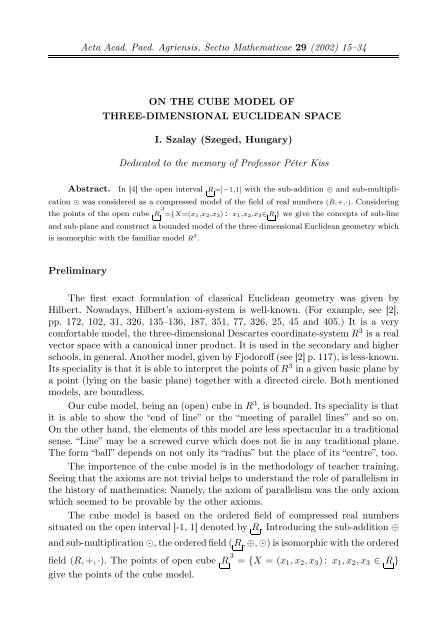
<strong>Acta</strong> <strong>Acad</strong>. <strong>Paed</strong>. <strong>Agriensis</strong>, <strong>Sectio</strong> <strong>Mathematicae</strong> <strong>29</strong> (<strong>2002</strong>) <strong>15–34</strong><br />
ON THE CUBE MODEL OF<br />
THREE-DIMENSIONAL EUCLIDEAN SPACE<br />
I. Szalay (Szeged, Hungary)<br />
Dedicated to the memory of Professor Péter Kiss<br />
Abstract. In [4] the open interval R =]−1,1[ with the sub-addition ⊕ and sub-multiplication<br />
⊙ was considered as a compressed model of the field of real numbers (R,+,·). Considering<br />
the points of the open cube R 3 ={X=(x 1,x 2,x 3) : x 1,x 2,x 3∈ R } we give the concepts of sub-line<br />
and sub-plane and construct a bounded model of the three dimensional Euclidean geometry which<br />
is isomorphic with the familiar model R 3 .<br />
Preliminary<br />
The first exact formulation of classical Euclidean geometry was given by<br />
Hilbert. Nowadays, Hilbert’s axiom-system is well-known. (For example, see [2],<br />
pp. 172, 102, 31, 326, 135–136, 187, 351, 77, 326, 25, 45 and 405.) It is a very<br />
comfortable model, the three-dimensional Descartes coordinate-system R 3 is a real<br />
vector space with a canonical inner product. It is used in the secondary and higher<br />
schools, in general. Another model, given by Fjodoroff (see [2] p. 117), is less-known.<br />
Its speciality is that it is able to interpret the points of R 3 in a given basic plane by<br />
a point (lying on the basic plane) together with a directed circle. Both mentioned<br />
models, are boundless.<br />
Our cube model, being an (open) cube in R 3 , is bounded. Its speciality is that<br />
it is able to show the “end of line” or the “meeting of parallel lines” and so on.<br />
On the other hand, the elements of this model are less spectacular in a traditional<br />
sense. “Line” may be a screwed curve which does not lie in any traditional plane.<br />
The form “ball” depends on not only its “radius” but the place of its “centre”, too.<br />
The importence of the cube model is in the methodology of teacher training.<br />
Seeing that the axioms are not trivial helps to understand the role of parallelism in<br />
the history of mathematics: Namely, the axiom of parallelism was the only axiom<br />
which seemed to be provable by the other axioms.<br />
The cube model is based on the ordered field of compressed real numbers<br />
situated on the open interval ]-1, 1[ denoted by R. Introducing the sub-addition ⊕<br />
and sub-multiplication ⊙, the ordered field (R, ⊕, ⊙) is isomorphic with the ordered<br />
field (R, +, ·). The points of open cube R 3 = {X = (x 1 , x 2 , x 3 ): x 1 , x 2 , x 3 ∈ R }<br />
give the points of the cube model.
16 I. Szalay<br />
Introduction<br />
Having the compression function u ∈ R ↦→ th u ∈] − 1, 1[ ([1], I. 7.54–7.58) we<br />
say that the compressed of u is given by the equation<br />
(0.1) u = thu, u ∈ R.<br />
Hence, we have that the compresseds of real numbers are just on the open interval<br />
R =] −1, 1[. Considering the compression function as an isomorphism between the<br />
fields (R, +, ·) and (R,⊕, ⊙) we define the sub-addition and sub-multiplication by<br />
the identities<br />
(0.2) u ⊕ v := u + v , u, v ∈ R<br />
and<br />
(0.3) u ⊙ v := u · v , u, v ∈ R,<br />
respectively. If x = u and y = v , then (0,1), (0,2) and (0,3) yield the relations<br />
(0.4) x ⊕ y = x + y<br />
1 + xy , x, y ∈ R<br />
and<br />
(0.5) x ⊙ y = th((arth x)(arth y)), x, y ∈ R.<br />
Moreover, we can use the identities<br />
(0.6) u ⊖ v := u − v , u, v ∈ R<br />
(0.7) u ○: v := u : v , u, v ∈ R, v ≠ 0<br />
or<br />
(0.8) x ⊖ y = x − y<br />
1 − xy , x, y ∈ R<br />
and<br />
( arth x<br />
)<br />
(0.9) x ○: y = th , x, y ∈ R, y ≠ 0,<br />
arthy
On the cube model of three-dimensional Euclidean space 17<br />
where the operations ⊖ and ○: are called sub-subtraction and sub-division, respectively.<br />
The inverse of compression is explosion defined by the equation<br />
(0.10)<br />
| |<br />
x = arthx, x ∈ R<br />
and<br />
| |<br />
x is called the exploded of x. Clearly, by (0.1) and (0.10) we have the identities<br />
| |<br />
(0.11) x = ( x ), x ∈ R<br />
and<br />
(0.12) u =<br />
|<br />
|<br />
(u) , u ∈ R.<br />
1. Operations on R 3<br />
Having the familiar three dimensional Euclidean vector-space R 3 with the<br />
traditional operations (addition, multiplication by scalar, inner product) as well as<br />
the concepts of norm and metric, we give their isomorphic concepts for R 3 which<br />
is the set of points X = (x 1 , x 2 , x 3 ) such that x 1 , x 2 , x 3 ∈ R. Clearly, R 3 forms<br />
an open cube in R 3 . Considering the vectors X = (x 1 , x 2 , x 3 ) and Y = (y 1 , y 2 , y 3 )<br />
from R 3 we define sub-addition as<br />
(1.1) X ⊕ Y = (x 1 ⊕ y 1 , x 2 ⊕ y 2 , x 3 ⊕ y 3 ),<br />
sub-multiplication by scalar c ∈ R as<br />
(1.2) c ⊙ X = (c ⊙ x 1 , c ⊙ x 2 , c ⊙ x 3 )<br />
and sub-inner product as<br />
(1.3) X ⊙ Y = (x 1 ⊙ y 1 ) ⊕ (x 2 ⊙ y 2 ) ⊕ (x 3 ⊙ y 3 ).<br />
Introducing the exploded of the point X = (x 1 , x 2 , x 3 ) as<br />
(1.4)<br />
| |<br />
| | |<br />
X = (<br />
|x 1 ,<br />
|x 2 ,<br />
|x 3 ), X ∈ R 3
18 I. Szalay<br />
and the compressed of the point U = (u 1 , u 2 , u 3 ) as<br />
(1.5) U = (u 1 , u 2 , u 3 ), U ∈ R 3<br />
we have the identities<br />
| |<br />
(1.6) X = ( X ), X ∈ R 3<br />
and<br />
(1.7) U =<br />
|<br />
|<br />
(U ) , U ∈ R 3 .<br />
Using (0.11), (0.2), (1.5) and (1.4), the identity (1.1) yields<br />
(1.8) X ⊕ Y =<br />
| |<br />
X +<br />
| |<br />
Y , X, Y ∈ R 3 .<br />
Moreover, by (0.11), (0.3), (1.4) the identity (1.2) yields<br />
(1.9) c ⊙ X =<br />
| |<br />
c ·<br />
| |<br />
X , c ∈ R and X ∈ R 3 .<br />
Considering the operations (1.1) and (1.2) we have the following<br />
Theorem 1.10. R 3 is a real vector space with the sub-addition (1.1) and scalar<br />
sub-multiplication (1.2). In detail, we have the following identities:<br />
(1.11) X ⊕ Y = Y ⊕ X, X, Y ∈ R 3 ,<br />
(1.12) (X ⊕ Y ) ⊕ Z = X ⊕ (Y ⊕ Z), X, Y, Z ∈ R 3 ,<br />
(1.13) X ⊕ o = X, where X ∈ R 3 arbitrary and o = (0, 0, 0),<br />
(1.14)<br />
X ⊕ (−X) = o, where − X<br />
is the familiar additive inverse of x ∈ R 3 .<br />
Moreover, the identities<br />
(1.15) 1 ⊙ X = X, X ∈ R 3 ,
On the cube model of three-dimensional Euclidean space 19<br />
(1.16) c ⊙ (X ⊕ Y ) = (c ⊙ X) ⊕ (c ⊙ Y ), c ∈ R, X, Y ∈ R 3 ,<br />
(1.17) (c 1 ⊕ c 2 ) ⊙ X = (c 1 ⊙ X) ⊕ (c 2 ⊙ X), c 1 , c 2 ∈ R, x ∈ R 3 ,<br />
(1.18) (c 1 ⊙ c 2 ) ⊙ X = c 1 ⊙ (c 2 ⊙ X), c 1 , c 2 ∈ R X ∈ R 3 ,<br />
also hold.<br />
Remark 1.19. By Theorem 1.10 we say that R 3 is a sub-linear space with the<br />
operations (1.1) and (1.2).<br />
Using (0.11), (0.3), (0.2) and (1.4) the identity (1.3) yields<br />
(1.20) X ⊙ Y =<br />
| |<br />
X ·<br />
| |<br />
Y , X, Y ∈ R 3 ,<br />
where “·” means the familiar inner product (of vectors<br />
For the sub-inner product we have<br />
| |<br />
X and<br />
| |<br />
Y ) in R 3 .<br />
Theorem 1.21. R 3 in a Euclidean vector space with the sub-inner product defined<br />
by (1.3) such that the sub-inner product has the following properties<br />
(1.22) X ⊙ Y = Y ⊙ X, X, Y ∈ R 3 ,<br />
(1.23) (X ⊕ Y ) ⊙ Z = (X ⊙ Z) ⊕ (Y ⊙ Z), X, Y, Z ∈ R 3<br />
(1.24) (c ⊙ X) ⊙ Y = c ⊙ (X ⊙ Y ), c ∈ R, X, Y ∈ R 3<br />
and for any X ∈ R 3 the inequality<br />
(1.25) X ⊙ X ≥ 0 holds such that X ⊙ X = 0 if and only if X = 0.<br />
Remark 1.26. By Theorem 1.21 we say that R 3 is a sub-euclidean space with the<br />
sub-inner product (1.3).
20 I. Szalay<br />
In [4] the concept of sub-function was defined for one variable (see [4], (0.8)<br />
and (0.9)). Hence, we have the sub-square root function<br />
(1.27) sub √ x =<br />
√<br />
| |<br />
x , x ∈ [0, 1).<br />
Having the property (1.25) and using the sub-square root function we can define<br />
the sub-norm as follows:<br />
(1.28) ‖X‖ R<br />
3 = sub √ X ⊙ X, x ∈ R 3 .<br />
Using (1.27), (1.20) and (0.12) the definition (1.28) yields<br />
| |<br />
(1.<strong>29</strong>) ‖X‖ 3 = ‖ X ‖ R R 3 , x ∈ R 3 ,<br />
where ‖ · ‖ R 3 means the familiar norm of vectors.<br />
Remark 1.30. Applying the familiar Cauchy’s inequality by (1.20), (0.1), (0.3)<br />
and (1.<strong>29</strong>) we have the inequality<br />
|X ⊙ Y | ≤ ‖X‖ R<br />
3 ⊙ ‖Y ‖ R<br />
3, X, Y, ∈ R 3 .<br />
Corollary 1.31. The sub-norm has the following properties<br />
(1.32) ‖X‖ R<br />
3 ≥ 0, (X ∈ R 3 ) such that‖X‖ R<br />
3 = 0 if and only if X = 0,<br />
(1.33) ‖c ⊙ X‖ R<br />
3 = |c| ⊙ ‖X‖ R<br />
3, c ∈ R, X ∈ R 3<br />
and<br />
(1.34) ‖X ⊕ Y ‖ R<br />
3 ≤ ‖X‖ R<br />
3 ⊕ ‖Y ‖ R<br />
3, X, Y ∈ R 3 .<br />
Remark 1.35. By Corollary 1.31 we say that R 3 is a sub-normed space with the<br />
sub-norm (1.28).<br />
Finally, we define the sub-distance of elements of R 3 as follows<br />
(1.36) d R<br />
3(X, Y ) = ‖X ⊖ Y ‖ R<br />
3, X, Y ∈ R 3 ,
On the cube model of three-dimensional Euclidean space 21<br />
where the sub-subtraction of vectors is defined by<br />
(1.37) X ⊖ Y = X ⊕ (−Y ).<br />
Using (1.<strong>29</strong>), (1.37), (1.8), (1.7), (1.4) and (0.10) the definition (1.36) yields<br />
| | | |<br />
(1.38) d 3(X, Y ) = d R R 3( X , Y ), X, Y ∈ R 3 ,<br />
where d R 3 is the familiar distance of the points of R 3 .<br />
Corollary 1.39. The sub-distance has the following properties<br />
(1.40) d R<br />
3(X, Y ) = d R<br />
3(Y, X), X, Y ∈ R 3 ,<br />
(1.41) d R<br />
3(X, Y ) ≥ 0 such that d R<br />
3(X, Y ) = 0 if and only if<br />
and<br />
X = Y, X, Y ∈ R 3<br />
(1.42) d R<br />
3(X, Y ) ≤ d R<br />
3(X, Z) ⊕ d R<br />
3(Z, Y ), X, Y, Z ∈ R 3 .<br />
Remark 1.43. By Corollary 1.39 we say that R 3 is a sub-metrical space with the<br />
sub-distance (1.36).<br />
2. On the geometry of R 3<br />
Our starting point is the Euclidean geometry of R 3 with its points, lines and<br />
planes based on the axioms formulated by Hilbert. Now we construct the cubemodel<br />
of the classical Euclidean geometry. The points of the model will be the<br />
points of R 3 . Considering a line l in R 3 its compressed will be the set of compressed<br />
points of l denoted by l. Considering a plane s in R 3 its compressed will be the<br />
set of compressed points of s denoted by s. The set λ = l is called sub-line and<br />
the set σ = s is called sub-plane. Clearly, λ ⊂ R 3 and σ ⊂ R 3 . Moreover, the<br />
exploded of a sub-line is a line and the exploded of a sub-plane is a plane, that is<br />
| |<br />
λ<br />
= l and<br />
| |<br />
σ<br />
= s.
22 I. Szalay<br />
By the axioms of the euclidean geometry of R 3 we have the properties of the<br />
geometry of R 3 .<br />
Denoting by L the set of lines of R 3 , by P the set of planes of R 3 , (R 3 ,L,P)<br />
is a so-called incidence geometry (see [3]). Considering L = {l : l ∈ L} and<br />
P = {s : s ∈ P}, (R 3 , L, P) is also an incidence geometry. Now we give the<br />
properties of “incidence”.<br />
Property 2.1. If X and Y are distinct points of R 3 then there exists a sub-line<br />
λ that contains both X and Y<br />
Property 2.2. There is only one λ such that X ∈ λ and Y ∈ λ.<br />
Property 2.3. Any sub-line has at least two points. There exist at least three<br />
points not all in one sub-line.<br />
Property 2.4. If X, Y and Z not are in the same sub-line then there exists a<br />
sub-plane σ such that X, Y and Z are in σ. Any sub-plane has a point at least.<br />
Property 2.5. If X, Y and Z are different non sub-collinear points, there is exactly<br />
one sub-plane containing them.<br />
Property 2.6. If two points lie in a sub-line, then the line containing them lies in<br />
the plane.<br />
Property 2.7. If two sub-planes have a joint point then they have another joint<br />
point, too.<br />
Property 2.8. There exists at least four points such that they are not on the same<br />
sub-plane.<br />
We will say that the point Z is between the points X and Y on the sub-line<br />
|<br />
|<br />
|<br />
|<br />
|<br />
Y<br />
|<br />
λ if Z is between X and on the line λ . The concept of “between” has the<br />
following properties:<br />
Property 2.9. If Z is between X and Y then X, Y and Z are three different points<br />
of a sub-line and Z is between Y and X.<br />
Property 2.10. For any arbitrary point X and Y there exists at least one point<br />
Z lying on the sub-line determined by X and Y such that Z is between X and Y .<br />
Property 2.11. For any three points of a sub-line there is only one between the<br />
other two.<br />
Property 2.12. (Pasch-type property.) If X, Y and Z are not in the same sub-line<br />
and λ is a sub-line of the sub-plane determined by the points X, Y and Z such<br />
that λ has not points X, Y or Z but it has a joint point with the sub-segment XY<br />
of the sub-line determined by X and Y then λ has a joint point with one of the<br />
sub-segmentes XZ or Y Z of the sub-lines determined by X and Z or Y and Z,<br />
respectively.<br />
We will say that two sets in R 3 are sub-congruent if their explodeds are<br />
congruent in the familiar sense. Let two half-lines be given with the same starting<br />
point W and let be U and V their inner points. Let us consider the familiar convex<br />
| |
On the cube model of three-dimensional Euclidean space 23<br />
angle ∡ UWV . Compressing this angle we obtain the sub-angle sub ∡ U W V<br />
(or sub-angle sub ∡ XZY where X = U , Y = V and Z = W ) with the peak-point<br />
W and bordered by the sub-half-lines determined by the points W , U and W ,<br />
V . The concept of “sub-congruence” and “sub-angle” have the following properties<br />
Property 2.13. On a given sub-half-line there always exists at least one subsegment<br />
such that one of its end-points is the starting point of the sub-half-line<br />
and this sub-segment is sub-congruent with an earlier given sub-segment.<br />
Property 2.14. If both sub-segments p 1 and p 2 are sub-congruent with the subsegments<br />
p 3 then p 1 and p 2 are sub-congruent.<br />
Property 2.15. If sub-segment p 1 is sub-congruent with sub-segment q 1 and p 2 is<br />
sub-congruent with q 2 then p 1 ∪ p 2 is sub-congruent with q 1 ∪ q 2 .<br />
Property 2.16. On a given side of a sub-half-lines there exists only one sub-angle<br />
which is sub congruent with a given sub-angle. Each sub angle is sub-congruent<br />
with itself.<br />
Property 2.17. Let us consider two sub-triangles. If two sides and sub-angles<br />
enclosed by these sides are sub-congruent in the sub-triangles mentioned above<br />
then they have another sub-congruent sub-angles.<br />
|<br />
We say that the sub-lines λ 1 and λ 2 are sub-parallel if their explodeds<br />
|λ 1 and<br />
| |λ 2 are parallel lines in the familiar sense. Now we have<br />
Property 2.18. If a sub-line λ 1 and a point X are given such that X is off λ 1<br />
then there exists only one sub-line λ 2 through X that is sub-parallel to λ 1 .<br />
Finally, we mention two properties for continuity.<br />
Property 2.19. (Archimedes-type property.) If a point X 1 is between the points<br />
X and Y on a sub-line then there are points X 2 X 3 , . . . , X n such that the subsegments<br />
X i−1 X i ; (i = 2, 3, . . .,n) are sub-congruent with sub-segment XX 1 and<br />
Y is between points X and X n .<br />
Property 2.20. (Cantor-type property.) If {X n Y n } ∞ n=1 is a sequence of subsegments<br />
lying on a sub-line λ such that for any n = 1, 2, 3, . . ., X n+1 Y n+1 ⊂ X n Y n<br />
then there exists at least one point Z of λ such that Z belongs to each X n Y n .<br />
To measure the sub-segments and sub-angles we can use the principle of<br />
isomorphic expressed by the identities (1.8), (1.9) and (1.20). If the sub-segment p<br />
has the end-points X and Y then its sub-measure can be defined as follows:<br />
(2.21) sub measp = meas<br />
| |<br />
p ,<br />
where meas<br />
| |<br />
p<br />
segment bordered by<br />
is understood in the traditional sense. Considering that<br />
| |<br />
X and<br />
| |<br />
Y we have that<br />
| |<br />
p<br />
is a<br />
meas<br />
| |<br />
| | | |<br />
p = D R 3( X , Y ).
24 I. Szalay<br />
Hence, by (2.21) and (1.38) we have<br />
(2.22) sub measp = d R<br />
3(X, Y ),<br />
which is the sub-distance of X and Y .<br />
Similarly, to measure sub-angles we write<br />
(2.23) sub meassub ∡XZY = meas ∡<br />
| | | | | |<br />
X Z Y<br />
|<br />
| |<br />
| |<br />
|<br />
where meas ∡ X Z Y is understood in the traditional sense. Using the concept<br />
of sub-function again, we obtain that<br />
(2.24) sub arccosx = arccos<br />
Moreover, we have the following<br />
| |<br />
x , x ∈ [−1, 1].<br />
Theorem 2.25. If X, Y and Z are given points of R 3 such that X ≠ Z and Y ≠ Z<br />
then<br />
(2.26)<br />
sub meassub ∡ XZY<br />
= sub arccos(((X ⊖ Z) ⊙ (Y ⊖ Z)) ○: (d R<br />
3(X, Z) ⊙ d R<br />
3(Y, Z))).<br />
3. Examples for special subsets of R 3<br />
Example 3.1. First, we show that the equation<br />
(3.2) X = B ⊕ (τ ⊙ M), τ ∈ R<br />
where B, M are given points of R 3 with the condition<br />
(3.3) ‖M‖ R<br />
3 = 1<br />
represents a sub-line. Really, using (1.8), (1.7) and (1.9) the equation (3.2) yields<br />
the equation<br />
(3.4)<br />
| |<br />
X =<br />
| | | |<br />
B + t M , t =<br />
| |<br />
τ ∈ R
On the cube model of three-dimensional Euclidean space 25<br />
which represents a line. Moreovoer, by (1.<strong>29</strong>) and (0.12) the condition (3.3) means<br />
that<br />
| |<br />
(3.5) ‖ M ‖ R 3 = 1<br />
holds. Writing that B = (b 1 , b 2 , b 3 ) and M = (m 1 , m 2 , m 3 ), the equation (3.2) is<br />
equivalent to the equation-system<br />
x 1 = b 1 ⊕ (τ ⊙ m 1 )<br />
x 2 = b 2 ⊕ (τ ⊙ m 2 ), τ ∈ R<br />
x 3 = b 3 ⊕ (τ ⊙ m 3 )<br />
which considering (0.4) and (0.5) can be written in the following form<br />
(3.6)<br />
(3.7)<br />
x 1 = b 1 + th((arth τ)(ar thm 1 ))<br />
1 + b 2 th((ar thτ)(ar th m 1 ))<br />
x 2 = b 2 + th((arth τ)(ar thm 2 ))<br />
, (−1 < τ < 1)<br />
1 + b 2 th((ar thτ)(ar th m 2 ))<br />
x 3 = b 3 + th((arth τ)(ar thm 3 ))<br />
1 + b 3 th((ar thτ)(ar th m 3 )) .<br />
In the special case B = ( 0, 0, 1 2<br />
( ) 1√6<br />
x 1 = th arthτ<br />
)<br />
and M =<br />
(<br />
th 1 √<br />
6<br />
, th 1 √<br />
6<br />
, th 2 √<br />
6<br />
)<br />
then (3.6) is<br />
( ) 1√6<br />
x 2 = th arthτ , −1 < τ < 1<br />
( )<br />
1 + 2 th √2<br />
6<br />
arthτ<br />
x 3 = ( )<br />
2 + th<br />
2√<br />
6<br />
arthτ<br />
and the sub-line is shown in the following figure:<br />
Fig. 3.8
26 I. Szalay<br />
Example 3.9. The sub-line given by the equation-system (3.7) (see Fig. 3.8) and<br />
the sub-line given by the equation-system<br />
) 1√6<br />
x 1 = th(<br />
arthτ<br />
(3.10)<br />
) 1√6<br />
x 2 = th(<br />
arthτ , −1 < τ < 1<br />
) 2√6<br />
x 3 = th(<br />
arthτ<br />
are sub-parallel and their graphs are shown in the following figure:<br />
Fig. 3.11<br />
Example 3.12. The sub-line given by the equation system (3.7) (see Fig. 3.8) and<br />
the sub-line given by the equation-system<br />
( ) 1<br />
x 1 = th √6 arth τ<br />
(3.13)<br />
( ) 1<br />
x 2 = − th √6 arthτ , −1 < τ < 1<br />
x 3 =<br />
( )<br />
1 + 2 th<br />
2√<br />
6<br />
arthτ<br />
( )<br />
2 + th<br />
2√<br />
6<br />
arth τ<br />
has the joint point B = ( 0, 0, 1 2)<br />
. Their graphs are shown in the following figure:<br />
Fig. 3.14
On the cube model of three-dimensional Euclidean space 27<br />
Example 3.15. The sub-lines given by (3.10) (see Fig. 3.11) and (3.13) (see Fig.<br />
3.14) have neither a joint point nor a joint sub-plane. They can be seen in the<br />
following figure<br />
Example 3.17. The equation<br />
Fig. 3.16<br />
(3.18) z = x ⊕ y ⊕ 1 2 , x, y ∈ R<br />
represents a sub-plane. Really, by (0.11) and (0.2) the computation<br />
| |<br />
| |<br />
z = x ⊕ y ⊕ 1 2<br />
= (<br />
x<br />
|<br />
|<br />
| |<br />
|<br />
) ⊕ ( y ) ⊕ (<br />
|( 1 2 ) ) =<br />
| |<br />
x +<br />
| |<br />
y<br />
|<br />
|<br />
⊕ (<br />
|( 1 2 ) )<br />
= (<br />
| |<br />
x +<br />
| |<br />
y +<br />
|<br />
| |( 1 2 ) ) =<br />
| |<br />
x +<br />
| | |<br />
y +( 1 2 )<br />
| |<br />
shows that if (x, y, z) satisfies (3.18) then the points ( x ,<br />
(0.4) the equation (3.18) is equivalent to the<br />
(3.19) z =<br />
so we have the surface of a sub-plane<br />
xy + 2x + 2y + 1<br />
, −1 < x, y < 1,<br />
2xy + x + y + 2<br />
| | | |<br />
y , z ) form a plane. By<br />
Fig. 3.20
28 I. Szalay<br />
The equation (3.19) shows that the sub-line (3.7) coincides with the sub-plane<br />
given by (3.18) . The Fig. 3.20 shows this fact.<br />
The sub-plane determined by the equation<br />
(<br />
(3.21) z = x ⊕ y = x + y )<br />
, x, y ∈ R<br />
1 + xy<br />
is sub-parallel with the sub-plane given by (3.18). Their surfaces are shown in the<br />
following figure:<br />
Fig. 3.22<br />
Fig. 3.22 shows that the sub-line (3.10) is on the sub-plane (3.21).<br />
Example 3.23. Considering the set<br />
(3.24) S X0 (ρ) = {X ∈ R 3 : d R<br />
3(X, X 0 ) = ρ, X 0 ∈ R 3 and ρ ∈ R + }<br />
by (1.38) and (0.12) we have<br />
| | |<br />
(3.25) d R 3( X ,<br />
|X 0 ) =<br />
| |<br />
|<br />
| |<br />
that is the points X ∈ R 3 form a sphere with centre X<br />
|0 and radius ρ . Therefore<br />
S X0 (ρ) is called a sub-sphere with centre X 0 and radius ρ. By (1.4), (3.25) and<br />
(0.10) we get the equation of sub-sphere<br />
| |<br />
ρ ,<br />
(3.26)<br />
(arthx − arthx 0 ) 2 + (arth y − arthy 0 ) 2 +<br />
+(arthz − arthz 0 ) 2 = (ar thρ) 2<br />
where X = (x, y, z) and X 0 = (x 0 , y 0 , z 0 ) are elements of R 3 .<br />
Although the sub-sphere is determined anambiguously by its centre and radius,<br />
its form depends on the place of the centre too. Moreover, it is not symmetrical in<br />
a traditional sense for its centre. The following figures show the sub-spheres<br />
S (1 ,1,1)<br />
(( 1 2 ) )<br />
, S (1 ,1,1) (1) and S (1 ,1,1) ((3 2 ))
On the cube model of three-dimensional Euclidean space <strong>29</strong><br />
having the equations<br />
(arthx − 1) 2 + (ar thy − 1) 2 + (arthz − 1) 2 = 1 4<br />
(arthx − 1) 2 + (ar thy − 1) 2 + (ar thz − 1) 2 = 1<br />
and<br />
(arthx − 1) 2 + (arthy − 1) 2 + (arthz − 1) 2 = 9 4 ,<br />
respectively<br />
Fig. 3.27<br />
Fig. 3.28<br />
Fig. 3.<strong>29</strong>
30 I. Szalay<br />
The sub-spheres S O (ρ) are symmetrical in a traditional sense for their centre<br />
o. By (3.26) the sub-sphere S 0 (ρ) has the following equation<br />
(3.30) (arthx) 2 + (arthy) 2 + (arthz) 2 = (arthρ) 2 .<br />
Considering now the sub-spheres S O (( 1 2 )), S O(1) and S o (( 3 2<br />
)) we obtain their<br />
equations by (3.30)<br />
(arthx) 2 + (arthy) 2 + (arthz) 2 = 1 4<br />
(arthx) 2 + (arthy) 2 + (arthz) 2 = 1<br />
and<br />
(arthx) 2 + (arthy) 2 + (arthz) 2 = 9 4<br />
and they are shown in the following figures:<br />
Fig. 3.31<br />
Fig. 3.32
On the cube model of three-dimensional Euclidean space 31<br />
Fig. 3.33<br />
4. Proof of Theorems<br />
4.1. Proof of Theorem 1.10. Considering that the verifications of identitites<br />
(1.11)–(1.14) are very similar, we give the proof of identity (1.12), only. After (1.8)<br />
and (1.7) we apply the familiar associativity of addition of vectors and using (1.7)<br />
and (18) again, we obtain:<br />
(X ⊕ Y ) ⊕ Z =<br />
|<br />
|<br />
X ⊕ Y +<br />
| |<br />
Z<br />
= (<br />
|<br />
| | | |<br />
X + Y ) +<br />
| |<br />
Z<br />
| |<br />
= ( X +<br />
| | | |<br />
Y ) + Z<br />
=<br />
| | | |<br />
X + ( Y +<br />
| |<br />
Z ) =<br />
|<br />
| | | | | |<br />
X + ( Y + Z )<br />
=<br />
| |<br />
X +<br />
|<br />
|<br />
Y ⊕ Z<br />
= X ⊕ (Y ⊕ Z).<br />
Considering that the verifications of identities (1.15)–(1.18) are very similar,<br />
we give the proof of identity (1.16), only. After (1.19), (1.8), and (1.7) we apply a<br />
familiar distributive property of multiplication of vectors by scalar and using (1.9)<br />
and (18) again, we get<br />
c ⊙ (X ⊕ Y ) =<br />
| | |<br />
|<br />
c ⊕ X ⊕ Y<br />
=<br />
| |<br />
c (<br />
|<br />
| | | |<br />
X + Y )<br />
=<br />
| |<br />
c<br />
| |<br />
( X +<br />
| |<br />
Y )<br />
=<br />
=<br />
| | | |<br />
c X +<br />
| |<br />
c ⊙ X +<br />
| | | |<br />
c Y<br />
= (<br />
| |<br />
c ⊙ Y<br />
|<br />
| | | |<br />
c X ) + (<br />
|<br />
| | | |<br />
c Y )<br />
= (c ⊙ X) ⊕ (c ⊙ Y ).<br />
4.2. Proof of Theorem 1.21. The verifications of identities (1.22)–(1.24) are<br />
very similar to the verifications mentioned above, so we prove the property (1.25),<br />
only. Using (1.20), (1.4) and (0.1)<br />
X ⊙ X =<br />
| |<br />
X ·<br />
| |<br />
X<br />
| |<br />
= th(( x1 )2 ) + (<br />
| |<br />
| |<br />
x2 )2 + ( x3 )2 ) ≥ 0
32 I. Szalay<br />
is obtained. Moreover, we have zero if and only if<br />
(0.10) means that X = O.<br />
| |<br />
X<br />
= O which by (1.4) and<br />
4.3. Proof of Theorem 1.31. The proof of property (1.32) is very similar to<br />
the proof of property (1.25), so we omit it. The identity (1.33) does not need new<br />
methods, so we accept it. We prove inequality (1.34). After (1.<strong>29</strong>), (1.8), (1.7) and<br />
(0.1) we apply the Minkowski-inequality and using (0.2) and (1.<strong>29</strong>), we can write<br />
|<br />
|<br />
| |<br />
‖X ⊕ Y ‖ 3 = ‖ X ⊕ Y ‖ R R 3 = ‖ X +<br />
| |<br />
Y ‖ R 3 ≤<br />
| |<br />
| |<br />
| |<br />
| |<br />
≤ ‖ X ‖ R 3 + ‖ Y ‖ R 3 = ‖ X ‖ R 3 ⊕ ‖ Y ‖ R 3 = ‖X‖ 3 ⊕ ‖Y ‖ 3. R R<br />
4.4. Proof of Theorem 1.39. Identity (1.40) is trivial, the verification of property<br />
(1.41) is easy, so we omit them. We verify the inequality (1.42), only. After (1.38)<br />
we use the triangular inequality and using (0.2) and (1.38) again, we have<br />
| | | |<br />
| | | |<br />
| | | |<br />
d 3(X, Y ) = d R R 3( X , Y ) ≤ d R 3( X , Z ) + d R 3( Z , Y ) =<br />
| | | |<br />
| | | |<br />
= d R 3( X , Z ) ⊕ d R 3( Z , Y ) = d 3(X, Z) ⊕ d 3(Z, Y ).<br />
R R<br />
4.5. Proof of Theorem 2.25. Our proof is based on the well-known inequality<br />
concerning the familiar angles enclosed by vectors. Namely,<br />
(U − W)(V − W) = d R 3(U, W) · d R 3(V, W)cos ∡ UWV<br />
where U, V, W ∈ R 3 such that U ≠ W and V ≠ W. Hence, denoting by U =<br />
V =<br />
| |<br />
Y and W =<br />
| |<br />
Z , we have<br />
| |<br />
X ,<br />
(4.6) meas ∡<br />
| | | | | |<br />
X Z Y = arccos<br />
| |<br />
( X −<br />
| | | |<br />
Z ) · ( Y −<br />
| |<br />
Z )<br />
.<br />
d R 3( | X | , | Z | ) · d R 3( | Y | , | Z | )<br />
| |<br />
Z =<br />
Applying (1.7), (1.8) and (1.37) we have that<br />
|<br />
|<br />
Y ⊖ Z hold. Hence (1.7) and (1.20) yield<br />
| |<br />
X −<br />
| |<br />
Z =<br />
|<br />
|<br />
X ⊖ Z and<br />
| |<br />
Y −<br />
| |<br />
(4.7) ( X −<br />
| | | |<br />
Z ) · ( Y −<br />
| |<br />
Z ) =<br />
|<br />
(X ⊖ Z) ⊙ (Y ⊖ Z) .<br />
|
On the cube model of three-dimensional Euclidean space 33<br />
On the other hand, by (0.12), (1.38), (0.12) again, (0.3) and (0.11) we have<br />
|<br />
|<br />
| | | |<br />
| | | |<br />
| | | |<br />
| | | |<br />
d R 3( X , Z ) · d R 3( Y , Z ) = (d R 3( X , Z )) · (d R 3( Y , Z ))<br />
=<br />
|<br />
|<br />
d 3(X, Y ) · R<br />
|<br />
|<br />
|<br />
d 3(Y, Z) = ( | d 3(x, Y ) | · |<br />
d 3(Y, Z) | )<br />
R R R<br />
= ( | d 3(X, Z) | |<br />
|<br />
) ⊙ ( d 3(Y, Z) ) =<br />
R R<br />
|<br />
|<br />
d 3(X, Z) ⊙ d 3(Y, Z) .<br />
R R<br />
|<br />
Hence, by (4.7), (0.12), (0.7) and (0.11) we can write<br />
| |<br />
( X −<br />
| | | | | |<br />
Z ) · ( Y − Z )<br />
=<br />
d R 3( | X | , | Z | ) · d R 3( | Y | , | Z | )<br />
|<br />
|<br />
(X ⊖ Z) ⊙ (Y ⊖ Z)<br />
|<br />
dR 3(X, Y ) ⊙ d R<br />
3(Y, Z) |<br />
=<br />
(<br />
(<br />
| |<br />
(X ⊖ z) ⊙ (Y ⊖ Z) )<br />
) |<br />
|<br />
d 3(X, Z) ⊙ d 3(Y, Z)<br />
R R<br />
|<br />
= (<br />
|<br />
|<br />
|<br />
|<br />
(X ⊖ Z) ⊙ (Y ⊖ Z) ) ○: ( d 3(X, Z) ⊙ d 3(Y, Z) )<br />
R R<br />
|<br />
=<br />
|<br />
((X ⊖ Z) ⊙ (Y ⊖ Z)) ○: (d 3(X, Z) ⊙ d 3(Y, Z)) .<br />
R R<br />
|<br />
Returning to (4.6) we obtain that<br />
= arccos<br />
meas ∡<br />
holds. Hence, (2.23) and (2.24) yield<br />
= arccos<br />
| | | | | |<br />
X Z Y<br />
|<br />
|<br />
((X ⊖ Z) ⊙ (Y ⊖ Z)) ○: (d 3(X, Z) ⊙ d 3(Y, Z))<br />
R R<br />
sub meassub ∡ XZY<br />
|<br />
|<br />
((X ⊖ Z) ⊙ (Y ⊖ Z)) ○: (d 3(X, Z) ⊙ d 3(Y, Z))<br />
R R
34 I. Szalay<br />
= sub arccos(((X ⊖ Z) ⊙ (Y ⊖ Z)) ○: (d R<br />
3(X, Z) ⊙ d R<br />
3(Y, Z))),<br />
that is, we have (2.26).<br />
References<br />
[1] Császár Ákos: Valós analízis. Tankönyvkiadó, Budapest, 1983.<br />
[2] Matematikai kislexikon (Editor in chief M. Farkas), Műszaki Könyvkiadó 3.<br />
kiadás, 1979.<br />
[3] Radó Ferenc és Orbán Béla: A geometriai mai szemmel. Dacia Kiadó,<br />
Kolozsvár, 1981.<br />
[4] Szalay I., On the compressed Descartes-plane and its applications, AMAPN<br />
17 (2001), 37–46.<br />
Szalay István<br />
Department for Matehamatics<br />
Juhász Gyula Teacher Training College<br />
University of Szeged<br />
6701 Szeged, P. O. Box 396.<br />
Hungary<br />
E-mail: szalay@jgytf.u-szeged.hu

![77–87 ALMOST SURE FUNCTIONAL LIMIT THEOREMS IN Lp(]0, 1 ...](https://img.yumpu.com/35912399/1/180x260/77-87-almost-sure-functional-limit-theorems-in-lp0-1-.jpg?quality=85)