On the GE Lattice Boltzmann Problem - SERC

A priori derivation of lattice Boltzmann equations for rotating fluids
Paul J. Dellar ∗
Department of Applied Mathematics and Theoretical Physics,
University of Cambridge, Silver Street, Cambridge CB3 9EW, UK †
(Dated: Submitted 16th October 2000, Revised: 8th December 2001)
Lattice Boltzmann equations suitable for simulating the rotating incompressible Navier-Stokes
equations are constructed from the continuum Boltzman equation. The Boltzmann equation in a
rotating frame contains a velocity-dependent Coriolis force term, unlike the velocity-independent
potential forces considered previously. The microscopic velocity dependence of the equilibrium distribution
and Coriolis force is expanded in Hermite polynomials and truncated consistently. In
particular, a higher order contribution from the Coriolis force eliminates an otherwise spurious
term in the viscous stress due to the leading order Coriolis contribution. A modified distribution
function is introduced to construct a fully explicit second order scheme that does not require additional
“spin” steps. Extension to the rotating shallow water and planetary geostrophic equations is
straightforward. Numerical experiments are presented for flow in a rotating channel.
PACS numbers: 05.20.Dd 51.10.+y 47.11.+j 92.10.Ei
I. INTRODUCTION
Methods based on lattice Boltzmann equations (LBE) are a promising alternative to conventional numerical methods
for simulating fluid flows [1]. Lattice Boltzmann methods are straightforward to implement and have proved especially
effective for simulating flows in complicated geometries, and for exploiting parallel computer architectures. For
these reasons, Salmon [2, 3] has recently advocated the use of lattice Boltzmann methods in oceanography. Most
oceanographic and atmospheric flows are strongly influenced by the Earth’s rotation [4, 5], and so require a lattice
Boltzmann scheme that incorporates the Coriolis force present in a rotating frame fixed to the Earth. By contrast,
the centrifugal force is usually negligible in geophysical applications.
The compressible Navier-Stokes equations in a frame rotating with constant angular velocity Ω, neglecting the
centrifugal force, are
∂ t ρ + ∇· (ρu) = 0,
∂ t (ρu) + ∇· (pI + ρuu) + 2ρΩ×u = ∇·(2µS),
(1a)
(1b)
where the viscous stress has been written in terms of the dynamic viscosity µ and strain tensor S. For an ideal
monatomic gas, S αβ = 1 2 (∂ αu β + ∂ β u α − 2 3 δ αβ∇·u), so that S αα = 0 in three dimensions. We follow [1] in using
Greek indices for vector components, reserving Roman indices for labelling discrete velocity vectors. The relative
importance of the viscous stress is denoted by the Reynolds number Re = uL/ν, where L is some lengthscale of the
flow and ν = µ/ρ is the kinematic viscosity. The term 2ρΩ×u is the Coriolis force. In geophysical applications, Ω is
often taken to be just the component of the angular velocity parallel to the local gravity vector, and thus varies with
latitude over the surface of a sphere [4, 5].
Lattice Boltzmann equations are most commonly used to simulate nearly incompressible flows, with Mach number
Ma = |u|/c s ≪ 1, where c s is the sound speed. Solutions of Eqs. (1a-b) then approximate solutions of the
incompressible Navier-Stokes equations,
∇· u = 0, (2a)
∂ t u + u · ∇u + ρ −1
0 ∇p + 2Ω×u = ν∇2 u. (2b)
Density variations are negligible in this limit, ρ = ρ 0 + O(Ma 2 ), so Eq. (1a) implies that ∇·u = O(Ma 2 ). Most lattice
Boltzmann equations adopt an isothermal equation of state, p = c 2 s ρ with constant sound speed c s [1, 6, 7]. This
changes the viscous stress to 2µS αβ = µ(∂ α u β + ∂ β u α ). In other words, an isothermal fluid possesses a bulk viscosity
∗ Electronic address: pdellar@na-net.ornl.gov
† Now at: OCIAM, Mathematical Institute, 24–29 St Giles’, Oxford, OX1 3LB, UK

µ ′ = (2/3)µ as well as a shear viscosity µ [8]. Since ∇·u = O(Ma 2 ), this difference becomes negligible in the low
Mach number limit.
The derivation of the Navier-Stokes equations from the continuum Boltzmann equation in a rotating frame has
caused considerable controversy in the past [9–13]. Although the correct rotating Navier-Stokes equations are obtained
at the first two orders in the Chapman-Enskog perturbation expansion based on a small mean free path (see Sec. II),
higher order momentum and heat transport terms are affected by the Coriolis force [9, 10]. However, it is to be
expected that the properties of a material rotating with respect to an inertial frame will be affected by the influence
of Coriolis and centrifugal forces on the material’s microscopic dynamics. These perturbations are proportional to
the inverse molecular Ekman number E −1 d = 2Ωd 2 /ν, where d is the mean free path [12]. While E −1 d is very small
for most real materials, where d is comparable with the molecular spacing, the same is not necessarily true for lattice
Boltzmann models, since d is the lattice spacing, and nor is it necessarily true for suspensions of particles in a viscous
fluid [12]. However, numerical experiments indicate that the lattice Boltzmann equation does demonstrate the correct
continuum behaviour, even in fairly unsuitable parameter regimes of modest Reynolds numbers and Mach numbers.
A lattice Boltzmann equation (LBE) is a discrete velocity model of the continuum Boltzmann equation designed
to reproduce the necessary structure that leads to the Navier-Stokes equations. Although LBEs were originally
constructed empirically as extensions of lattice gas automata (LGA) [14, 15] to continuous distribution functions
[7, 16], it was later realised that the most common isothermal LBEs correspond to systematic truncations of the
continuum Boltzmann equation in velocity space based on tensor Hermite polynomials [17–20]. This construction
leads to particular expressions for the discrete equilibrium distributions, whereas the moment constraints necessary
to reproduce the Navier-Stokes equations usually leave at least one undetermined function [2, 3, 20, 21]. In two
dimensions, the Euler equations impose six constraints (one scalar, one vector, one symmetric tensor) which is precisely
right for schemes based on hexagonal lattices, as used in [14–16, 22–24]. For the now more common nine speed lattice
illustrated in Fig. 1, this leaves three undetermined functions. Two are constrained by the form of the viscous stress,
and the ninth constraint is need to suppress a grid-scale density instability [25]. For general equations of state this
stability criterion gives different equilibria to those obtained by the above Hermite truncation, but they coincide for
isothermal fluids.
A velocity-space truncation of the continuum Boltzmann equation was also used [26–30] to incorporate a body force
ρA in the Navier-Stokes momentum equation,
∂ t (ρu) + ∇· (pI + ρuu) = ρA + ∇·(2µS). (3)
In this previous work the body force was velocity independent, and moreover the gradient of a potential. This body
force was intended to simulate a more realistic equation of state than a perfect monatomic gas. Lattice Boltzmann
simulations of incompressible flow driven by pressure gradients, for instance flow through porous media [1, 31],
often use body forces instead because a true pressure gradient would require an unreasonably large density gradient.
Moreover, lattice Boltzmann equations typically remains stable for higher Reynolds numbers when the flow is driven
by a body force instead of a pressure gradient [32].
In the current work A will be a generic body force except where particular properties of the Coriolis force ρA =
−2ρΩ×u are indicated. The Coriolis force has been dealt with before [2, 3, 24], but these previous treatments suffer
from an incorrect viscous stress due to their discrete form of the body force. In particular, they do not simulate
rotating Poiseuille flow correctly (see Sec. IX). This error is in addition to the usual ∇·(ρuuu) error arising from an
equilibrium truncated at O(u 2 ) in the most commond unforced lattice Boltzmann equations [6] that may be corrected
by employing more particle speeds [33, 34].
Lattice gases with body forces that are linear in the particle velocities, notably the Coriolis force, were considered
previously in [15]. Since lattice gas populations, and hence momenta, are restricted to discrete values, the authors of
[15] proposed a stochastic redistribution of populations at each lattice point designed to produce the correct average
momentum change. This forcing scheme does not appear to have been implemented, although a similar stochastic
approach for velocity-independent forcing was tested in [22].
2
II.
THE BOLTZMANN EQUATION WITH A BODY FORCE
The continuum Boltzmann-BGK equation with a body force is [35–37],
∂ t f + ξ · ∇f + a · ∇ ξ f = − 1 τ (f − f (0) ), (4)
where f(x, ξ, t) is the single-particle distribution function, and ξ the microscopic particle velocity. The third term on
the left hand side is the acceleration a applied to each particle by external forces, where the lower case a indicates

a possible dependence on the microscopic velocity ξ. For the Coriolis force, this acceleration is a = −2Ω×ξ. While
most derivations of the continuum Boltzmann equation explicitly exclude velocity-dependent body forces, heuristic
justifications for this particular body force may be found in [36] for the mathematically equivalent Lorentz force
exerted on charged particles by a uniform magnetic field, and in [10]. They rely on the fact that ∇ ξ · a = 0, so
a · ∇ ξ f = ∇ ξ · (af) for all f. A systematic derivation of Eq. (4) from the Liouville equation in a rotating frame via
the Bogoliubov-Born-Green-Kirkwood-Yvon (BBGKY) hierarchy [35, 38] is given in appendix A.
The right hand side of Eq. (4) uses the Bhatnagar-Gross-Krook (BGK) approximation [39] to Boltzmann’s original
binary collision term, in which f relaxes towards a Maxwell-Boltzmann equilibrium distribution f (0) with a single
relaxation time τ. This equilibrium is
( )
f (0) ρ
=
(2πθ) exp (ξ − u)2
− , (5)
3/2 2θ
where ρ, u and θ are the dimensionless macroscopic density, velocity and temperature, in units where the particle
masses and Boltzmann’s constant are both unity. Velocities are scaled so that the isothermal sound speed c s = θ 1/2 .
The three macroscopic quantities in Eq. (5) are defined by moments of the distribution function f,
∫
∫
ρ = fdξ, ρu = ξfdξ, ρθ = 1 ∫
|ξ − u| 2 fdξ, (6)
3
where the integrals with respect to ξ are taken over all of R 3 . For given ρ, u and θ, the Maxwell-Boltzmann
distribution minimises the Boltzmann entropy functional H = ∫ f ln(f)dξ. The simplified BGK collision term on the
right hand side of Eq. (4), like Boltzmann’s original binary collision term, drives the distribution function f towards a
local Maxwell-Boltzmann equilibrium f (0) while conserving the local density, momentum, and temperature (internal
energy). These properties are sufficient to reproduce the Navier-Stokes equations [35–38, 40]. The Navier-Stokes
equations also involve two other macroscopic quantities, the stress (or momentum flux density) tensor Π, and the
equilibrium stress tensor Π (0) , given by the second order moments,
∫
∫
Π = ξξfdξ, Π (0) = ξξf (0) dξ = θρI + ρuu. (7)
3
The trace of Π (0) gives the equation of state p = θρ = c 2 s ρ. Only the trace of the stress tensor is conserved by the
collision term on the right hand side of Eq. (4), and the difference Π − Π (0) gives rise to a viscous stress.
A. Chapman-Enskog expansion
The Navier-Stokes equations with a body force may be derived from moments of the continuum Boltzmann equation
in the limit of slow variations in space and time via a Chapman-Enskog expansion. Although the Chapman-Enskog
expansion itself appears widely in the literature [1, 35–38, 40], the necessary modifications for a body force, and
especially a velocity dependent body force, seem to be less readily accessible. In particular, the usual Navier-Stokes
viscous stress emerges from subtle cancelations between three different terms.
The Chapman-Enskog expansion introduces a small parameter ɛ into the collision time, so that Eq. (4) becomes
∂ t f + ξ · ∇f + a · ∇ ξ f = − 1
ɛτ (f − f (0) ). (8)
Thus spatial and temporal derivatives appear at lower order in ɛ than the collision term, corresponding to slowly
varying solutions. The parameter ɛ may be identified physically with the dimensionless mean free path, or Knudsen
number, but its main purpose is to sidestep the moment closure problem that plagues hydrodynamic turbulence.
By assuming a particular form for the solution, only moments of the known equilibrium distribution f (0) and their
derivatives in space and time appear [40].
The Chapman-Enskog expansion poses a multiple scale expansion of both f and t in powers of ɛ,
f = f (0) + ɛf (1) + ɛ 2 f (2) + · · · , ∂ t = ∂ t0 + ɛ∂ t1 + · · · , (9)
where t 0 and t 1 are advective and diffusive timescales respectively, with the solvability conditions
∫
∫
f (n) dξ = 0, and ξf (n) dξ = 0, for n = 1, 2, . . . . (10)

Thus the higher order terms f (1) , f (2) , . . . do not contribute to the macroscopic density or momentum. These constraints
determine evolution equations for the macroscopic quantities. For simulating low Mach number flows it
∫ is convenient to impose a constant temperature, θ = θ 0 is constant, instead of the the extra solvability condition
|ξ − u| 2 f (n) dξ = 0 for n = 1, 2, . . . that would yield an evolution equation for θ. These two approaches agree to
O(Ma 2 ), the discrepancy being a bulk viscous stress proportional to ∇·u as analysed in [8].
Substituting these expansions into the Boltzmann equation (8), we obtain
(∂ t0 + ξ · ∇ + a · ∇ ξ ) f (0) = − 1 τ f (1) , (11a)
4
∂ t1 f (0) + (∂ t0 + ξ · ∇ + a · ∇ ξ ) f (1) = − 1 τ f (2) ,
(11b)
at O(1) and O(ɛ). The leading order continuity and momentum equations, Eqs. (1a) and (3) with ν = 0, follow from
the first two moments of Eq. (11a),
∫
∂ t0 ρ + ∇· (ρu) + ∇ ξ · (af (0) )dξ = 0,
(12a)
∫
∂ t0 (ρu) + ∇·Π (0) + ξ∇ ξ · (af (0) )dξ = 0,
(12b)
where ρ, u and Π (0) are defined in Eqs. (6) and (7). The right hand sides vanish by virtue of the solvability conditions
in Eq. (10). These two equations are equivalent to the Euler equations for an inviscid rotating fluid, equations (1a,b)
with ν = 0, since the first two moments (1, ξ) of the Coriolis term are 0 and 2ρΩ×u respectively (see Appendix C).
In the non-isothermal case an evolution equation for the temperature would result from multiplying Eqs. (11a,b) by
|u − ξ| 2 and integrating over ξ [8, 35, 36].
At next order in ɛ, from Eq. (11b) and the solvability conditions, we obtain
∫
∂ t1 ρ + ∇ ξ · (af (1) )dξ = 0,
(13a)
∫
∂ t1 (ρu) + ∇·Π (1) + ξ∇ ξ · (af (1) )dξ = 0.
(13b)
The body force term in Eq. (13a) vanishes, being an exact divergence, so the correct continuity equation (1a) is
recovered to the first two orders in ɛ. Similarly, the third term in Eq. (13b) vanishes from the solvability conditions
(see Appendix B).
The stress Π (1) = ∫ ξξf (1) dξ is given, from the ξξ moment of Eq. (11a), by
[
(∫ ) ∫
]
Π (1) = −τ ∂ t0 Π (0) + ∇· ξξξf (0) dξ + ξξ∇ ξ · (af (0) )dξ , (14)
that reduces (see Appendix B) to the Newtonian viscous stress Π (1)
αβ
= −θτρ (∂ αu β + ∂ β u α ). The multiple scales
expansion in time determines ∂ t0 Π (1) via the known quantities ∂ t0 ρ and ∂ t0 (ρu). Thus if τ = ν/θ the viscous
Navier-Stokes momentum equation (3) is recovered from the continuum Boltzmann equation at this order. The
disappearance of the body force from the stress Π (1) relies upon an exact cancelation between the last term in
Eq. (14) and a contribution to ∂ t0 Π (0) from the body force appearing in the leading order momentum equation.
B. Moments of the body force
∫ The above derivation of the Navier-Stokes equations with a body force contains the moments ρ, ρu, Π (0) , and
ξξξf (0) dξ of the equilibrium distribution. The body force term a∇ ξ f = ∇ ξ · (af) also only appears via its
moments, the first three (1,ξ,ξξ) moments given by
∫
∇ ξ · (af (0) )dξ = 0,
(15a)
∫
ξ∇ ξ · (af (0) )dξ = −ρA,
(15b)
∫
ξξ∇ ξ · (af (0) )dξ = −ρ(Au + uA),
(15c)

where A is the macroscopic acceleration due to the body force. For velocity-independent body forces A = a. For the
velocity-dependent Coriolis force, a = −2Ω×ξ and A = −2Ω×u as expected.
In previous work [26–29] the acceleration a did not depend upon the microscopic velocity ξ, so the required three
moments (15a-c) followed automatically from an integration by parts and the use of Eq. (6). Moreover, these moments
held for all distributions f, not just for the equilibrium distribution f (0) . In appendix C we show that these three
moments of ∇ ξ · (af (0) ) do also hold for the Coriolis force. However, the second moment equation (15c) does not
hold for general distribution functions f, so the Coriolis force contributes to the so-called Burnett terms. These are
higher order corrections to the Navier-Stokes equations arising from f (2) and higher terms in the Chapman-Enskog
expansion [9, 10].
5
III.
BOLTZMANN EQUATION WITH DISCRETE VELOCITY SPACE
The above derivation of the rotating Navier-Stokes equations from the continuum Boltzmann equation (4) via
the Chapman-Enskog expansion requires the first four moments (1, ξ, ξξ, ξξξ) of the equilibrium distribution f (0) ,
and the first three moments (1, ξ, ξξ) of the body force a · ∇ ξ f (0) . The lattice Boltzmann philosophy restricts the
microscopic velocity ξ to a discrete set {ξ 0 , . . . , ξ N }, and replaces f(x, ξ, t) by a discrete set of functions f i (x, t),
while reproducing the moment structure of the continuum Boltzmann equation as closely as possible In particular the
macroscopic variables, now given by the discrete moments
N∑
N∑
N∑
ρ = f i , ρu = ξ i f i , Π = ξ i ξ i f i , (16)
i=0
i=0
should satisfy the same Navier-Stokes equations as the continuum moments in the last section when the f i evolve
according to the lattice Boltzmann equation
i=0
∂ t f i + ξ i · ∇f i = − 1 τ (f i − f (0)
i ) + R i , for i = 0, . . . , N. (17)
The body force term a · ∇ ξ f has been replaced by some source terms R i . The Chapman-Enskog expansion of
Sec. II proceeds slightly differently if R i depends only upon the macroscopic ρ and u, since a · ∇ ξ f (0) is replaced by
−R i = −R (0)
i , and the a · ∇ ξ f (n) vanish for n = 1, 2, . . .. The analogues of (11a,b) are
(∂ t0 + ξ i · ∇)f (0)
i = − 1 τ f (1)
i + R i , (18a)
∂ t1 f (0) + (∂ t0 + ξ i · ∇)f (1)
i = − 1 τ f (2)
i , (18b)
so the explicit a · ∇ ξ f (1) body force terms in (13a,b) that were shown to vanish in appendix B are now absent. The
required constraints on f (0)
i and R i are thus (from Eqs. 6, 7, 15a-c)
N∑
i=0
f (0)
i = ρ,
N∑
i=0
ξ i f (0)
i
= ρu,
N∑
i=0
ξ i ξ i f (0)
i = θρI + ρuu, (19)
N∑
i=0
ξ α ξ β ξ γ f (0)
i = ρu α u β u γ + θρ (u α δ βγ + u β δ γα + u γ δ αβ ) , (20)
N∑
R i = 0,
i=0
N∑
ξ i R i = ρA,
i=0
N∑
ξ i ξ i R i = ρ(Au + uA). (21)
i=0
The ρu α u β u γ term in Eq. (20) is often dropped, being O(Ma 3 ), as explained in Appendix B.
In order to motivate the following calculations, many previous lattice Boltzmann schemes with body forces have
implicitly set the second moment in Eq. (15c) or Eq. (21) to zero, removing the last term in Eq. (14). These schemes
therefore produce the incorrect viscous stress
Π (1) = −τθρ [ ∇u + (∇u) T] − τρ(uA + Au). (22)

6
6
2
5
3
0
1
7
4
8
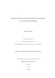
FIG. 1: The nine particle speeds in the 2D square lattice. Integrating the lattice Boltzmann equation along a characteristic for
a timestep ∆t in Sec. VI is equivalent to moving particles from one lattice point to another.
Luo [26, 27] drew attention to the second moment Eq. (15c) of the continuum body force, and observed that most
previous work had implicitly set the analogous discrete moment to zero. However, Luo [26, 27] seemed to have been
motivated only by a desire for a truncation order consistent with the usual moment expansion of the equilibrium
distribution (see Sec. IV), and did not exhibit a concrete error in previous work comparable to the second term in
Eq. (22).
No unexpected effects are visible in forced Poiseuille flow, the most common test problem [32, 41, 42], because
the spurious stress has zero divergence. In this geometry the spurious stress −τρ(Au + uA) = (−2τρAu)ŷŷ, ŷ
being a unit vector in the streamwise direction. The divergence of this stress vanishes because τ, ρ, u and A are all
independent of the streamwise coordinate y. By contrast, the velocity profile for rotating Poiseuille flow with the
most common body force term, as in [2, 3, 24], deviates from the expected parabola (see Sec. IX) by an amount in
agreement with the deviation due to the second term in Eq. (22).
IV.
UNFORCED NINE SPEED LATTICE BOLTZMANN EQUATION
The most common scheme in two dimensions uses nine particle speeds arranged on a square lattice as shown in
Fig. 1. Equations (19) impose six constraints on the nine discrete equilibria f (0)
i , and the form of the viscous stress
imposes only two more. This leaves one undetermined function that must be chosen to suppress a grid-scale density
instability [25]. Although this is not how it was originally constructed, the most common nine speed lattice Boltzmann
scheme for isothermal fluids [7] coincides with a systematic truncation of the continuum Boltzmann equation in velocity
space [17, 18], and this is the procedure we use below. However, it should be pointed out that this procedure leads
to unstable schemes for other barotropic equations of state like the shallow water equations [25], even though the
shallow water equations also have a continuum kinetic formulation [43, 44].
In the low Mach number limit, |u| ≪ c 2 s = θ, the exact Maxwell-Boltzmann distribution (5) may be expanded as
(
f (0) = ρw(ξ) 1 + ξ · u
)
(ξ · u)2
+
θ 2θ 2 − u2
+ O(u 3 ), (23)
2θ
where w(ξ) is the weight function
w(ξ) = (2πθ) −D/2 exp ( −ξ 2 /2θ ) . (24)
As explained in appendix D, this series expansion in u is equivalent to retaining the first three terms in an expansion
of the Maxwell-Boltzmann distribution in tensor Hermite polynomials [17, 18, 45], the coefficients being given by

the moments in Eqs. (6). These Hermite polynomials are mutually orthogonal with respect to the weighted inner
product defined by the Gaussian weight function w(ξ). The ρu α u β u γ term in Eq. (20) disappears to this order of
approximation.
Each moment of this approximate f (0) that appears in the continuum theory now comprises the integral of a
polynomial p(ξ) of degree five or less in ξ multiplying the weight function w(ξ). These integrals may be evaluated
exactly using a Gaussian quadrature formula based on the Hermite polynomials,
∫
p(ξ) exp (−ξ 2 /2θ)dξ =
N∑
w i p(ξ i ), (25)
where the points ξ i are the quadrature points, and the coefficients w i are the corresponding weights [46]. It is sufficient
to use a three point Gaussian quadrature separately for the ξ x and ξ y coordinates [17, 18]. The quadrature points
form an integer lattice, with ξ x , ξ y ∈ {−1, 0, 1} as illustrated in Fig. 1, in units where θ = 1 3
. This is where the
isothermal (constant θ) approximation is needed to make the lattice vectors uniform in length.
The one dimensional weights { 1 3 , 2 3 , 1 3
} combine to give
⎧
⎪⎨ 4/9, i=0,
w i = 1/9, i=1,2,3,4,
(26)
⎪⎩
1/36, i=5,6,7,8,
and the discrete equilibria are [1, 7, 17, 18]
f (0)
i
= w i ρ
i=0
(1 + 3ξ i · u + 9 2 (ξ i · u) 2 − 3 2 u2 )
, (27)
from substituting ξ = ξ i and w(ξ) = w i in Eq. (23). Although the results follow from the above construction via
Gaussian quadratures, we may also verify that Eq. (27) has the required discrete moments given in Eqs. (19) and (20)
(albeit without the ρu α u β u γ term) with the aid of identities such as [21]
7
8∑
w i ξ i = 0,
i=0
8∑
w i ξ i ξ i = 1 3 I,
i=0
8∑
w i ξ i ξ i ξ i = 0. (28)
i=0
The equilibria in Eq. (27) are not the only ones with the necessary moments, Eqs. (19) and (20), but they are the
unique equilibria determined by the stability requirement in [25]. The fact that the truncated Hermite expansion
satisfies this requirement for an isothermal equation of state (only) appears to be coincidental.
The factorisation of the two-dimensional integral explains why we need nine speeds instead of the more obvious
five, namely four along the coordinate axes plus one rest particle. The extra diagonal speeds renders these lattice
Boltzmann equations genuinely multidimensional, whereas most conventional upwind schemes require further work in
more than one space dimension [47, 48]. There is also an alternative two-dimensional quadrature using an equilateral
triangular lattice, with speeds on the six vertices of a hexagon as in [14–16, 22–24], but numerical experiments suggest
that the nine speed square lattice remains stable at higher Reynolds numbers [21].
V. EXPANSION OF THE BODY FORCE
Luo [26] proposed using a similar low Mach number, or Hermite polynomial, expansion for the a · ∇ ξ f term,
a · ∇ ξ f = −ρw(ξ)θ −1 [ (ξ − u) + θ −1 (ξ · u)ξ ] · A + O(u 3 ), (29)
where A is assumed to be O(u). The coefficients of the expansion in u and ξ have been chosen so that the first
three moments of the right hand side Eq. (29) are exactly as in (15a-c). This formula may be derived by substituting
the moments from Eqs. (15a-c) as coefficients of an expansion in orthogonal Hermite polynomials, as indicated in
appendix D. A similar formula appeared in [29], though these authors chose a different weight function proportional
to exp(−ξ 2 /2) that ignored the θ dependence of the exponent in the Maxwell-Boltzmann distribution (see appendix
D). A discrete formula follows from substituting ξ = ξ i and w(ξ) = w i as for the equilibrium distribution above,
R i = −ρw i θ −1 [ (ξ i − u) + θ −1 (ξ i · u)ξ i
]
· A. (30)

Although Luo’s derivation relied upon a being independent of ξ, the formula (29) may also be used for the Coriolis
force,
and in discrete form
a · ∇ ξ f = ρw(ξ)θ −1 ( 1 + θ −1 ξ · u ) ξ · (2Ω×u) + O(u 3 ), (31)
R i = −ρw i θ −1 ( 1 + θ −1 ξ i · u ) ξ i · (2Ω×u), (32)
because the first three moments of a · ∇ ξ f (0) with the Coriolis force a = −2Ω×ξ still have the required form as in
Eqs. (15a-c). As with the discrete equilibria in Sec. IV, each of these formulas based on the Hermite expansion is only
one of many possibilities with the required moments. In two dimensions, Eqs. (15a-c) impose only six constraints on
the R i , but there are typically nine independent functions.
Luo [26] also noted that the simpler forcing term
a · ∇ ξ f = −ρw(ξ)θ −1 ξ · A + O(u 2 ), (33)
is often used [3, 24, 30, 42], and amounts to setting the second moment (15c) of the true forcing term a · ∇ ξ f to zero.
As shown in Sec. III this omission gives rise to a spurious contribution to the viscous stress as in Eq. (22). This may
also be seen in the energy equation derived from the trace of the second moment of the Boltzmann equation. The
trace of Eq. (14) gives (see [8] for details)
( 1
∂ t0
2 ρu2 + 3 ) ( 1
2 θρ + ∇·
2 ρu2 u + 5 )
2 θρu − ρA · u = − 1 2 TrΠ(1) , (34)
where −ρA · u on the left hand side accounts for the work done by the body force ρA. This term disappears when the
approximation (33) is used for the body force. Since Eq. (34) in fact contains no new information for an isothermal
fluid (because ∂ t0 ρ, ∂ t0 u, and ∂ t0 θ = 0 are already known) consistency with the momentum equation requires that
ρA · u appears in − 1 2 TrΠ(1) on the right hand side, in agreement with Eq. (22). For a thermal fluid the situation
is more serious, because the extra solvability condition TrΠ (1) = 0 turns Eq. (34) into an evolution equation for the
temperature θ (again, see [8] for details). Thus the work done by the body force that is not accounted for by the
missing −ρA · u term incorrectly goes into changing the internal energy or temperature.
In an alternative approach, He et al. [28] used the fact that the exact Maxwell-Boltzmann equilibrium distribution
(5) satisfies
8
to approximate the forcing term by
∇ ξ f (0) = − ξ − u f (0) , (35)
θ
a · ∇ ξ f ≈ a · ∇ ξ f (0) = −θ −1 a · (ξ − u)f (0) , (36)
or in discrete form
R i = −θ −1 a · (ξ i − u)f (0)
i . (37)
For the particular case of the Coriolis force, we may simply replace a by A = −2Ω×u in Eq. (36), due to the vector
identity (Ω×ξ) · (u − ξ) = (Ω×u) · (u − ξ). Using a small Mach number expansion of f (0) , the above expression
agrees with Luo’s formula (29) up to O(u 2 ). However, Eq. (36) contains additional terms of O(u 3 ) and higher that
are inconsistent with the truncation of f (0) at O(u 2 ).
Martys et al. [29] suggested that the ad hoc replacement of f by f (0) in Eq. (36) may be justified because the first
two Hermite coefficients of f and f (0) always coincide. In fact, the first three moments of Eq. (36) are correct,
∫
− θ −1 a · (ξ − u)f (0) = 0,
∫
− ξθ −1 a · (ξ − u)f (0) = −ρA, (38)
∫
− ξξθ −1 a · (ξ − u)f (0) = −ρ(Au + uA),

for a = A independent of ξ, provided f (0) is taken to be the exact Maxwell-Boltzmann distribution (5). If instead
f (0) is taken to be the approximate equilibrium distribution truncated at O(Ma 2 ), as in Eq. (23), the second moment
acquires a spurious extra term,
∫
− ξξθ −1 a · (ξ − u)f (0) = −ρ(Au + uA) − θ −1 ρ(A · u)uu. (39)
9
This extra term is only O(Ma 3 ) so the forcing term (36) is still an improvement on the simpler force in Eq. (33),
although not as good as Luo’s force (29). The divergence of the spurious stress in Eq. (39) typically vanishes for
channel flows of the form u = u(x)ŷ, such as Poiseuille or Couette flow, as considered in Sec. IX, and vanishes
identically for the Coriolis force because A · u = 0.
VI.
FULLY DISCRETE LATTICE BOLTZMANN EQUATION WITH BODY FORCE
Equation (17) must be approximated in x and t, as well as in ξ, to obtain a fully discrete lattice Boltzmann equation.
Integrating Eq. (17) along a characteristic for a time interval ∆t yields
f i (x + ξ i ∆t, t + ∆t) − f i (x, t) =
where the g i combine the collision and body force terms,
g i (˜x, ˜t) = − 1 τ
(
f i (˜x, ˜t) − f (0)
i
∫ ∆t
0
g i (x + ξ i s, t + s)ds, (40)
)
(˜x, ˜t) + R i (˜x, ˜t). (41)
A second order accurate numerical scheme requires a second order accurate quadrature, for instance the trapezium
rule,
∫ ∆t
0
g i (x + ξ i s, t + s)ds = ∆t (
)
g i (x + ξ
2
i ∆t, t + ∆t) + g i (x, t) + O(∆t 3 ). (42)
Unfortunately, g i (x+ξ i ∆t, t+∆t) is not known independently of the f i (x+ξ i ∆t, t+∆t), because f (0)
i and usually R i
depend implicitly on the f i via their moments, the macroscopic variables ρ and u. Thus a straightforward application
of Eq. (42) to Eq. (40) yields a set of coupled nonlinear algebraic equations for the f i at time t + ∆t.
He et al. [28, 30] observed that the combined equations (42) and (40) may be rendered fully explicit by a change
of variables. Introducing an alternative set of distribution functions f i defined by
f i (x, t) = f i (x, t) + ∆t
2τ
the scheme Eqs. (40) and (42) is algebraically equivalent to the fully explicit scheme
f i (x + ξ i ∆t, t + ∆t) − f i (x, t) =
(
)
f i (x, t) − f (0)
i (x, t) − ∆t
2 R i(x, t), (43)
τ∆t
τ + ∆t/2 R ∆t
(
)
i(x, t) −
f
τ + ∆t/2 i (x, t) − f (0)
i (x, t) . (44)
The macroscopic density, momentum and stress are readily reconstructed from moments of the f i ,
ρ =
8∑
f i , ρu =
i=0
8∑
i=0
ξ i f i + ∆t (
2 ρA, 1 + ∆t )
Π =
2τ
8∑
ξ i ξ i f i + ∆t
2τ Π(0) + ∆t ρ(Au + uA). (45)
2
In the absence of a body force, R i = 0, Eq. (44) is the usual form for a lattice Boltzmann equation, and resembles
a first order approximation to Eq. (40) except for the replacement of τ by τ + 1 2∆t [1]. However, it is perhaps not
always recognised that this simple replacement also implicitly replaces f i in the continuum equations with f i in the
discrete equations, and f i differs by O(∆t) from f i . So the strain field, for instance, is not given simply by Π − Π (0)
as it is in the continuum equations, where u and Π denote the ξ and ξξ moments of f i . For the Coriolis force, where
the macroscopic acceleration A = −2Ω×u itself depends on u, the second of Eqs. (45) may still be solved for u as
(
1 + ∆t 2 |Ω| 2) u = u − ∆tΩ×u + ∆t 2 u · ΩΩ. (46)
i=0

This simplifies to u = u − ∆tΩ×u + O(∆t 2 ), consistent with overall second order accuracy, but the exact expression
gave much smaller errors for fixed Ω∆t in numerical experiments.
Our proposed scheme thus comprises Eq. (44) for evolving the variables f i as defined at discrete lattice points.
The relaxation time is τ + ∆t/2, τ being chosen so that τθ = ν is the desired kinematic viscosity. The equilibrium
distribution f (0)
i and body force term R i , defined by Eqs. (27) and (32) respectively, are evaluated using u and ρ
computed from the moments of the f i via Eqs. (45). The original variables f i are no longer necessary. The combination
+ τ −1 R i may be regarded as defining a modified equilibrium distribution, one that transforms Eq. (44) into a
conventional lattice Boltzmann equation, except the modified BGK collision term fails to conserve momentum by
precisely the right amount to simulate the Coriolis force.
Similar variables f i − 1 2 ∆tR i were introduced previously in [41]. This treatment followed the opposite approach
of Taylor-expanding a postulated discrete equation like Eq. (44) to obtain a system of partial differential equations
(PDEs), rather than viewing Eq. (44) as a finite difference approximation to a known system of PDEs. They [41]
realised that a direct solution of Eq. (44) required an alternative expansion of the form
f (0)
i
f i = f (0)
i + ɛ(f (1)
i + g (1)
i ) + ɛ 2 (f (2)
i + g (2)
i ) + · · · , (47)
with f (1)
i , f (2)
i , . . . all taken to be independent of the body force. The solvability conditions in Eq. (10) applied only to
these functions, while g (1)
i was assumed to be linear in the body force, and subsequently found to be g (1)
i = − 1 2 ∆tR i.
Salmon [2] originally solved the combination of Eqs. (40) and (42) using a second order predictor-corrector scheme
to estimate f i (x + ξ i ∆t, t + ∆t) before evaluating the formula Eq. (42). In a subsequent paper, Salmon [3] noted that
this predictor-corrector scheme required many iterations to converge, especially in three dimensions, and proposed an
improved scheme. This revised scheme is equivalent to a second order Strang splitting [49, 50] that interleaves one
timestep of a conventional discretization of the unforced lattice Boltzmann equation,
∂ t f i + ξ i · ∇f i = − 1 τ (f i − f (0)
i ), (48)
between two half steps of solving ordinary differential equations for the Coriolis terms,
∂ t f i = R i = −3ρw i (1 + 3ξ i · u)ξ i · (2Ω×u). (49)
The two separate half steps are required to achieved global second order accuracy. As indicated below Eq. (45), the
unforced lattice Boltzmann equation (48) may be solved with second order accuracy by absorbing the O(∆t) error
into a redefinition of τ [1]. The ordinary differential equations (49) may be solved by first solving ∂ t u = A for u(t),
after which the right hand side becomes a known function of t that may be integrated. The additional 3ξ i · u in the
R i term renders Eq. (49) quadratic in u, so the integrated expression is more complicated than in [3].
10
VII.
PLANETARY GEOSTROPHIC AND UNSTEADY STOKES EQUATIONS
In geophysical fluid dynamics, the momentum equation (1b) is commonly nondimensionalised as
Ro [∂ t (ρu) + ∇·(ρuu)] + ∇p + ρ ˆΩ×u = E∇·(2ρS). (50)
The Rossby number Ro = u/(2ΩL) denotes the relative importance of inertial and Coriolis effects, where L is a
typical lengthscale and ˆΩ is a unit vector parallel to Ω. The Ekman number E = ν/(2ΩL 2 ) is the inverse Reynolds
number based on the Coriolis velocity scale 2ΩL. For large scale geophysical applications the Rossby number is often
sufficiently small that the inertial terms may be discarded, leaving the geostrophic momentum equation [4, 5],
∇p + ρ ˆΩ×u = E∇·(2ρS). (51)
This is usually combined with a Boussinesq equation for temperature to form the planetary geostrophic equations,
although the viscous term is often replaced or supplemented by an algebraic damping term such as −λρu [4, 5].
The ρuu term in Eq. (50), which comes from the ρuu term in the equilibrium stress Π (0) , may be removed [2, 3, 31]
by truncating the small Mach number expansion of the equilibrium distribution at O(u) instead of O(u 2 ), leading to
f (0)
i = w i ρ (1 + 3ξ i · u) , (52)

instead of Eq. (27). The lattice Boltzmann equation with this equilibrium distribution solves the rotating compressible
unsteady Stokes equations in the form
∂ t ρ + ∇· (ρu) = 0, (53)
∂ t (ρu) + ∇p + 2ρΩ×u = ∇·[ν(∇(ρu) + ∇(ρu) T )].
In principle the time derivative ∂ t (ρu) should also be discarded, since it is usually of comparable magnitude to the
∇·(ρuu) term, but this is not possible within the confines of an explicit lattice Boltzmann model.
While we still recover the rotating incompressible unsteady Stokes equations in the small Mach number limit, the
density gradient now enters the viscous stress at finite Mach numbers because it is no longer canceled by terms
previously present in ∂ t0 (ρuu). The ∇ρ terms may be eliminated using the leading order (inviscid) momentum
equation, but this now brings in extra terms proportional to ∂ t (ρu). Steady states will however be solutions of
∇p + 2ρΩ×u = ∇·(νρ [ ∇u + (∇u) T] ). (54)
provided the Coriolis force is included with the improved body force term Eq. (29). It is perhaps surprising that the
extra term in the body force is still needed, but this is because the viscous stress Π (1) only involves the time derivative
of the leading order stress Π (0) . Thus in a steady state the viscous stress is unchanged by the omission of the ∂ t0 ρuu
term in ∂ t0 Π (0) , and would still contain the spurious τρ(Au + uA) term.
11
VIII.
SHALLOW WATER EQUATIONS
The shallow water equations (SWE) are commonly used in geophysical fluid dynamics as a prototype for studying
phenomena like wave-vortex interactions present in more complex models. They model a thin layer of incompressible
fluid with a free surface, and are equivalent to the two dimensional compressible Navier-Stokes equations, with equation
of state p = 1 2 gρ2 , when the density ρ is identified with the layer height, rather than the (constant) density of the
fluid composing the layer [4, 5]. A nine speed SWE lattice Boltzmann formulation has been devised by Salmon [2].
The equilibrium distributions are
(
f (0) 9
0 = w 0 ρ
4 − 15 8 gρ − 3 )
2 u2 , (55)
( 3
2 gρ + 3ξ i · u + 9 2 (ξ i · u) 2 − 3 )
2 u2
f (0)
i
= w i ρ
for i ≠ 0,
with corresponding moments ρ, ρu and Π (0) = 1 2 gρ2 I + ρuu. Only the equation of state, and hence the constant term
in the expansion of f (0) in powers of u, differs from the isothermal Navier-Stokes distributions. However Eq. (55)
is not the truncated Hermite expansion with these moments. The truncated Hermite equilibria are unstable to a
grid-scale instability associated with the remaining degree of freedom that is not constrained by the eight moments
appearing in the Chapman-Enskog expansion [25].
The viscous force takes the unusual form [2, 25]
∇·Π (1) = −τθ [ ∇ 2 (ρu) + 2∇∇·(ρu) + O(Ma 2 /Fr 2 ) ] , (56)
where the Froude number Fr = u/ √ gρ is the ratio of the fluid speed to the surface gravity wave speed. The O(Ma 2 /Fr 2 )
term is due to the time derivative ∂ t0 Π (0) , and so vanishes for steady states. The cancelation of the density gradient
that gives a Newtonian viscous stress (see appendix B) does not occur with the shallow water equation of state (see
[25] for details). However, the O(Ma 2 /Fr 2 ) term is asymptotically smaller than the other terms in the normal lattice
Boltzmann limit of small Mach number, and may be made arbitrarily smaller by making the Mach number sufficiently
small, equivalent to taking sufficiently small timesteps.
The explicit lattice Boltzmann model constructed in the previous section works equally well for the rotating shallow
water equations if the previous discrete equilibrium distributions Eq. (27) are replaced by those in Eq. (55). Discarding
the O(u 2 ) terms from Eq. (55) gives a a planetary geostrophic form of the shallow water equations.
IX.
NUMERICAL EXPERIMENTS
We illustrate the discrepancy due to the simpe body force term Eq. (33) for simulating Poiseuille flow in a two
dimensional rotating channel. The flow is driven by a spatially uniform body force F ŷ directed along the channel,

12
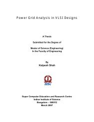
FIG. 2: Bounce back boundary conditions assign incoming population densities from points (gray circle) outside the boundary
(thick line) by reversing outgoing particles from points inside the boundary (black circle). The effective boundary (thick line)
is half way between lattice points.
and adopts a steady state depending only upon the cross-channel coordinate x. The dimensionless flow parameters,
low Reynolds number and moderate Mach number, are chosen to highlight the discrepancy due to the spurious body
force. The discrepancy is correspondingly smaller, though still present, in more common parameter regimes with
higher Reynolds numbers and lower Mach numbers.
A. Isothermal Navier-Stokes
Assuming ρ = ρ(x) and u = v(x)ŷ, the two-dimensional, isothermal Navier-Stokes equations (1a,b) simplify to
c 2 ∂ρ
s
∂x = 2ρΩv, −F = ∂ (
µ ∂v )
, (57)
∂x ∂x
where the isothermal equation of state is p = c 2 s ρ. The rotation axis is taken to be the z axis, so Ω = Ωẑ. No slip
boundary conditions are v(0) = v(1) = 0. Mass conservation requires ∫ 1
ρ(x)dx = 1 if the flow is assumed to have
0
developed from an initial state with unit density.
The analysis is greatly simplified if the dynamic viscosity µ is independent of the density ρ, as for a dilute monatomic
gas. This surprising result, subsequently verified experimentally, was one of the first successes of classical kinetic theory
[38]. To reproduce this property with the BGK approximation, for which ν = θτ and µ = ρθτ, it is necessary to take
τ ∝ ρ −1 , making τ a function of x and t instead of a constant. Fortunately, the analysis of Sec. VI and appendix B
is unchanged when τ = τ(x, t).
For constant µ, the fluid velocity is the usual parabolic Poiseuille profile v(x) = F x(1 − x)/(2µ), unaffected by
rotation. This flow gives rise to a Coriolis force in the cross-stream (x) direction that is balanced by a pressure and
density gradient, giving
( ΩF x 2 )
(3 − 2x)
ρ(x) = ρ 0 exp
6µc 2 . (58)
s
The constant ρ 0 is chosen so that ∫ 1
ρ(x)dx = 1, an integral that must be evaluated numerically.
0
The unsteady lattice Boltzmann scheme derived in Sec. VI was used to simulate a flow starting from rest with
uniform density ρ = 1. Rigid side walls were simulated using the “bounce back” boundary conditions [1, 21, 23, 41]
applied directly to the f i . For flow aligned with the lattice, these boundary conditions have the effect of placing the
rigid wall half a lattice spacing outside the lattice point at which they are applied, as illustrated in Fig. 2. This is
why the outermost data points in Figs. 3 and 4 do not coincide with the boundaries at x = 0, 1. Previous analyses
of these boundary conditions [32, 41] did not have additional R i forcing terms in the transformation (43) from f i to
f i , so the R i should perhaps be subtracted out before applying the bounce back boundary conditions. However, the
scheme as implemented did converge with second order spatial accuracy as expected.
The transformation from f i to f i giving a fully explicit lattice Boltzmann scheme also gives a relation Eq. (45) for
the fluid velocity u in terms of u = ∑ i ξ if i . For the body force ρA = F ŷ − 2ρΩ×u that itself depends on u, Eq. (45)

13
1
0.8
0.6
v
0.4
0.2
exact solution
simple force
Luo’s force
0
0 0.2 0.4 0.6 0.8 1
x
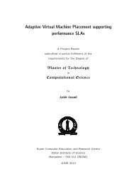
FIG. 3: The velocity profile for Ω = 50 computed using both the simple body force in Eq. (33) and Luo’s improved force in
Eq. (29). The former’s departure from the exact parabolic solution is clearly visible. The other parameters were µ = 0.05,
Ma = √ 3/20 ≈ 0.0866, F = 0.4, using 80 lattice points. Only some lattice points are shown for clarity.
1.1
exact solution
Luo’s force
1.05
ρ
1
0.95
0.9
0 0.2 0.4 0.6 0.8 1
x
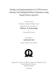
FIG. 4: The numerical density profile for Ω = 20 with body force from Eq. (29) compared with the exact solution Eq. (58).
For these parameters ρ 0 ≈ 0.9026. The grid used 80 points, only half of which are shown.
implies that
u = ( ū + ∆tΩ¯v + ∆t 2 ΩF/(2ρ) ) / ( 1 + ∆t 2 Ω 2) ,
v = (¯v − ∆tΩū + ∆tF/(2ρ)) / ( 1 + ∆t 2 Ω 2) ,
(59a)
(59b)
where u = (u, v, 0) and u = (ū, ¯v, 0). Numerical accuracy is improved by retaining the O(∆t 2 ) terms, although the
convergence remains formally second order if they are neglected.
Figure 3 shows the computed velocity profiles for Ω = 50 with the simple forcing, and with Luo’s improved forcing
Eq. (29). The parameters for the simulation in Figs. 3 and 4 were µ = 0.05, Ma = √ 3/20 ≈ 0.0866, F = 0.4, and

14
0.025
0.02
measured error
O(δ) approximation
0.015
0.01
0.005
∆ v
0
−0.005
−0.01
−0.015
−0.02
Ω=20 (Luo’s force)
Ω=5
Ω=10
Ω=20
−0.025
0 0.2 0.4 0.6 0.8 1
x
FIG. 5: Deviations from the parabolic exact solution for rotating Poiseuille flow. The deviation due to the use of the simple
body force, and its associated spurious stress, for Ω = 5 agrees well with the O(δ) approximation given by Eq. (61). The
agreement is less good at Ω = 20, since more terms in the series are required. The deviation for Ω = 20 using Luo’s force (- - -)
is not visible on this plot. All simulations used 80 lattice points, though for clarity not all points are shown.
80 lattice points, the particular values of F and µ being chosen to make the maximum speed u = 1 at x = 0.5. The
deviation from the exact parabolic profile due to the spurious stress in the simple forcing term Eq. (33) is clearly
visible. Figure 4 shows that the density from a numerical experiment with Ω = 20 and Luo’s forcing Eq. (29) agrees
well with the analytical expression in Eq. (58). The scaling constant is ρ 0 ≈ 0.9026 for these parameter values.
No detectable difference was found between the two different body forces in Eqs. (29) and (36), because the
divergence of the spurious stress at O(Ma 3 ) due to He et al.’s forcing Eq. (36) vanishes in a uniform channel. However,
Luo’s forcing term Eq. (29) is preferable because it lacks this spurious term completely. The extra term ∂ γ (ρu α u β u γ )
at O(Ma 3 ) in the viscous stress (see appendix B) also vanishes exactly for this geometry since u = vŷ and ∂ y = 0.
B. Isothermal Navier-Stokes with spurious stresses
The simple body force in Eq. (33) introduces a spurious stress µc −2
s (Au + uA) into the momentum equation. For a
channel geometry the divergence of this stress is µc −2
s ∂ x (A x v) = 4µc −2
s Ωv∂ x (v), so the modified continuum equations
are
(
c 2 ∂ρ
∂ 2
s
∂x = 2ρΩu, −F = µ v
∂x 2 + 4Ωc−2 s v ∂v )
. (60)
∂x
The latter equation unfortunately has no exact solution, but an asymptotic solution may be found by expanding v(x)
in the small parameter δ = ΩF/(µc 2 s ),
v(x) = F (
2µ x(1 − x) 1 + δ
)
30 (6x3 − 9x 2 + x + 1) + O(δ 2 ) . (61)
Figure 5 compares the difference between the numerical velocity profile using the simple force and the exact parabolic
solution with the O(δ) correction due to the spurious stress given by Eq. (61). It shows good agreement for Ω = 5
(δ = 0.3) but the agreement is less good for Ω = 20, for which more terms in the series in δ are needed. The streamwise
forcing F does not appear on the right hand side of Eq. (60), so no unexpected effects are visible in non-rotating
Poiseuille flow.

15
X. CONCLUSION
The hydrodynamic equations derived from the continuum Boltzmann equation in a rotating frame by the Chapman-
Enskog expansion correspond to the Navier-Stokes equations with a Newtonian viscous stress. The Coriolis force,
and more generally any body force, disappears from the viscous stress via a subtle cancelation of terms between the
macroscopic momentum equation and the second moment of the forcing term, Eq. (15c). Thus one extra moment of
the forcing term is required beyond that necessary to reproduce the correct leading order momentum equation, as it
appears in Eq. (14) for the viscous stress. Many previous lattice Boltzmann equations for forced flows neglect this
extra moment, and thus produce the erroneous viscous stress calculated in Eq. (22). This is in addition to the usual
∇·(ρuuu) contribution from using a truncated nine speed equilibrium [6] that may be corrected by employing more
particle speeds [33, 34].
The extra discrepancy was verified by simulating Poiseuille flow in a rotating channel, and precisely corresponds to
the calculated error in the viscous stress. Conversely, the forcing term suggested by Luo [26, 27] that retains one more
order in the small u expansion does give a correct viscous stress. No discrepancy is visible in non-rotating Poiseuille
flow because the spurious stress has zero divergence, and so has no effect on the velocity.
Although the Coriolis force in the continuum Boltzmann equation depends upon the microscopic particle velocity
as derived in Appendix A, unlike the forces in almost all previous work, but the resulting formulas Eqs. (32) and (37)
are identical to those that would be obtained for a force 2Ω×u instead of 2Ω×ξ.
While it might be argued that the spurious terms disappear anyway in the small Mach number and high Reynolds
number limit, since they are easily removed by a small modification to the body force there is no reason not to remove
them. Their removal will only improve the accuracy of numerical solutions at fixed Mach number and Reynolds
number, and their presence is enough to disrupt an attempt to demonstrate that a lattice Boltzmann scheme converges
to an intended exact solution, rather than to a solution of the wrong continuum equations as modified by the spurious
stress. This paper arose partly out of the author’s failure to establish that Salmon’s lattice Boltzmann scheme for the
shallow water equations [2, 3] converged to solutions obtained with conventional numerical methods.
Conversely, it is useful to have quantified the error due to the use of a simpler forcing term such as Eq. (33). For
instance, in lattice Boltzmann formulations of magnetohydrodynamics the magnetic field B is typically known at
lattice points, but its derivative J = ∇×B is not. Thus the Lorentz force J×B is most easily incorporated [51, 52]
by changing the second moment of the equilibrium to be
Π (0) = θρI + ρuu + 1 2 |B|2 I − BB. (62)
The last two terms comprise the Maxwell stress, with divergence −J×B since ∇·B = 0. Since the macroscopic
momentum equation now includes the Lorentz force, the viscous stress acquires an error −τ [(J×B)u + u(J×B)] as
in Eq. (22), but the necessary correction term cannot be written as the divergence of a stress. Fortunately the error
is only O(Ma 3 /Re) in the usual scaling with |B| 2 = O(ρ|u| 2 ) [52].
In another possible application, Verberg & Ladd [53] solved directly for steady states of the forced Stokes equations
using a linear system solver in conjunction with a lattice Boltzmann equation omitting the nonlinear u 2 terms from
the equilibria. The same approach could not be used to find zero Rossby number solutions of Eq. (50) with the forcing
term Eq. (32), because this term is quadratic in u even though the macroscopic term Coriolis force 2Ω×u itself is
linear. A simpler forcing term such as Eq. (33) would have to be used, with a corresponding error in the viscous stress
as calculated.
Finally, the particular formula (30) is just one of many with the required moments given by Eqs. (15a-c). These
moments impose only six constraints in two dimensions, but most lattice Boltzmann schemes use more than six
particle speeds. Some stability criterion may be needed to determine the forcing terms R i uniquely, like that in [25]
for unforced nine-speed equilibria. The need for such criteria is more acute in schemes for simulating thermal flows.
These typically use 13 or more speeds in two dimensions [1, 33, 34] so there are many more as yet undetermined
degrees of freedom.
Acknowledgments
The author thanks Rick Salmon for useful conversations and advance copies of his papers, and Stephane Zaleski for
a useful conversation. Some of this work was undertaken at the 2000 Summer Study Program in Geophysical Fluid
Dynamics at Woods Hole Oceanographic Institution, supported by ONR and NSF. Financial support from St John’s
College, Cambridge, UK is gratefully acknowledged.

16
APPENDIX A: DERIVATION OF THE BOLTZMANN EQUATION FROM THE LIOUVILLE EQUATION
IN A ROTATING FRAME
Most derivations of the Boltzmann equation explicitly exclude velocity-dependent body forces like the Coriolis force
[35, 38]. A heuristic justification for the Boltzmann equation with a Coriolis force was given by Woods [10], and by
Chapman & Cowling [36] for the mathematically equivalent Lorentz force exerted on charged particles by a uniform
magnetic field. In this appendix we outline a more systematic derivation from the Liouville equation in a rotating
frame via the Bogoliubov-Born-Green-Kirkwood-Yvon (BBGKY) hierarchy [35, 38]. Such a derivation has been given
previously by Delcroix [54] in a French language summer school proceedings, again for charged particles in a uniform
magnetic field, but we have been unable to locate a more acccessible treatment. Our approach follows that of Huang
[35] and Uhlenbeck & Ford [38] as modified by a rotating frame.
The equation of motion for a single particle of mass m moving with velocity ξ under a potential Φ in a frame
rotating with angular velocity Ω is
( )
dξ
m
dt + 2Ω×ξ = − ∂Φ
∂x .
(A1)
The potential Φ(x) may include a centrifugal term 1 2 m|Ω×x|2 , but this is usually negligible in geophysical applications.
This equation may be put in Hamiltonian form using the canonical variables q = x and p = m(ξ + R), where R(x)
is any vector field satisfying ∇×R = 2Ω. In geophysical fluid dynamics the combination p = m(u − fy, v + fx, w)
is often used, for 2Ω = fẑ, and goes by the name “geostrophic momentum.” This change of variables may be more
familiar for the Lorentz force, with R = A being a vector potential for the magnetic field B = 2Ω [55]. The single
particle Hamiltonian is the total energy as seen in the rotating frame,
H 1 = 1 2 m|ξ|2 + Φ(x) = 1
2m |p|2 − p · R + ˜Φ(q),
in terms of p and q, where ˜Φ = Φ + 1 2 m|R|2 . Hamilton’s equations are [4, 56]
(A2)
The left hand side of Eq. (A3b) is
dq α
dt
dp α
dt
= ∂H 1
∂p α
= 1 m p α − R α = ξ α , (A3a)
= − ∂H 1
∂q α
= − ∂ ˜Φ
∂q α
+ p β
∂R β
∂q α
.
(A3b)
dp α
dt
= m d dt (ξ α + R α ) = m dξ α
dt + m∂R α
· dq β
∂q β dt = mdξ α
dt + ∂R α
(p β − mR β ),
∂q β
(A4)
from which Eq. (A3b) may be rearranged to coincide with Eq. (A1),
m dξ α
dt = mξ β
( ∂Rβ
− ∂R )
α
− ∂Φ = [2mξ×Ω − ∇Φ]
∂x α ∂x β ∂x α
.
α
(A5)
Next consider a system of N identical such particles, each with position q i and canonical momentum p i = m(ξ i +R),
where i = 1, . . . , N. We assume the Hamiltonian is of the form
H =
N∑
i=1
1
2m |p i − mR| 2 +
N∑
i=1
Φ(q i ) + ∑ i

Denoting the 6 coordinates (q i , p i ) by z i for brevity, the N-particle density function D(z 1 , . . . , z N ) satisfies Liouville’s
equation, [35, 36, 38, 40, 55]
dD
dt = ∂D
N ∂t + ∑
[
˙q i · ∂D + ṗ i · ∂D ] [ ∂
=
∂q i ∂p i ∂t + h N (z 1 , . . . , z N )]
D = 0,
i=1
that expresses conservation of volume in the 6N dimensional phase space. The structure of Eq. (A9) is unmodified by
the Coriolis force, only the definition of the p i has changed [55]. The Hamiltonian operator h N (z 1 , . . . , z N ) is given
by
17
(A9)
h N (z 1 , . . . , z N ) =
N∑
i=1
∂H
∂p i
·
∂
− ∂H ·
∂q i ∂q i
∂
∂p i
=
N∑
S i + 1 ∑
P ij ,
2
i=1
i≠j
(A10)
where the single and multi-particle contributions are
( ) (
1 ∂
S i =
m p iα − R α +
∂q iα
∂R β
p iβ − ∂ ˜Φ
)
∂q iα ∂q iα
(
∂
∂
, P ij = K ij · −
∂p iα ∂p i
∂ )
. (A11)
∂p j
The rotating frame introduces extra terms involving R into S i , but the Hamiltonian operator may still be rewritten
in divergence form, so that
h N (z 1 , . . . , z N )D =
The Hamiltonian operator may be decomposed into
N∑
i=1
(
∂
· D ∂H )
−
∂ (
· D ∂H )
. (A12)
∂q i ∂p i ∂p i ∂q i
h N (z 1 , . . . , z N ) = h s (z 1 , . . . , z s ) + h N−s (z s+1 , . . . , z N ) +
s∑
N∑
i=1 j=s+1
for s = 1, . . . , N − 1, and we observe, after integration by parts using the divergence form Eq. (A12), that
∫
dz s+1 · · · dz N h N−s (z s+1 , . . . , z N )D(z 1 , . . . , z N ) = 0.
P ij ,
(A13)
(A14)
Thus substituting the decomposition Eq. (A13) into the Liouville equation and integrating over z s+1 · · · z N causes the
term involving h N−s (z s+1 , . . . , z N ) to vanish, leaving the Bogoliubov-Born-Green-Kirkwood-Yvon (BBGKY) hierarchy
(see [35, 36, 38] for references)
( ∂
∂t + h s)
f s (z 1 , . . . , z s ) = −
s∑
∫
dz s+1 K i,s+1 ·
i=1
∂
∂p i
f s+1 (z 1 , . . . , z s+1 ),
for the reduced s particle distribution functions f s defined by
∫
N!
f s (z 1 , . . . , z s , t) =
dz s+1 · · · dz N D(z 1 , . . . , z N ).
(N − s)!
Each equation in the hierarchy comprises a streaming operator (∂ t + h s ) acting on the the s particle distribution
function f s , and a collision term depending on f s+1 . This is the usual moment closure problem. However, the hope
is that the right hand sides, denoting simultaneous interactions (“collisions”) involving two, three, four, and so on
particles, become successively less important for a sufficiently dilute gas [35, 36, 38].
The first equation, s = 1, is
( ( )
∂ 1
∂t + m p 1α − R α
The partial derivatives transform as
(
∂ ∂R β
+ p 1β − ∂ ˜Φ
)
∂q 1α ∂q 1α ∂q 1α
) ∫
∂
f 1 = −
∂p 1α
dz 2 K 12 ·
∂
∂p 1
f 2 (z 1 , z 2 , t).
(A15)
(A16)
(A17)
( ∂
∂q 1α
)p
( ∂
=
∂x α
)ξ
( ) ( ∂Rβ ∂
−
,
∂x α ∂ξ β
)x
( ∂
=
∂p 1α
)q 1 ( ∂
, (A18)
m ∂ξ α
)x

under the change of variables x = q 1 , ξ = m −1 p 1 − R, bringing the left hand side of Eq. (A17) into the form of the
Boltzmann equation with a Coriolis force,
( ∂
∂t + ξ ∂
α − 1 (
∂Φ ∂ ∂Rβ
+ ξ β − ∂R ) ) ∫
α ∂
∂
f 1 = − dx 2 dξ
∂x α m ∂x α ∂ξ α ∂x α ∂x β ∂ξ 2 K 12 · f 2 (z 1 , z 2 , t). (A19)
α ∂ξ 1
The collision operator on the right hand side of Eq. (A19) is unaffected by the Coriolis force, since the potential φ
in K 12 is independent of ξ, and no R terms appear in the transformation relating ∂/∂p 1 and ∂/∂ξ. The collision
operator may be shown to coincide with the usual Boltzmann binary collision term for spatially uniform systems
[35, 38, 40, 55].
The Boltzmann streaming operator may always be written in divergence form using canonical (q 1 , p 1 ) variables by
observing that the left hand side takes the form
( ∂
∂t + ∂H 1
∂p 1
·
∂
∂q 1
− ∂H 1
∂q 1
·
)
∂
f 1 = ∂f 1
∂p 1 ∂t +
∂ ( )
∂H 1
· f 1 −
∂q 1 ∂p 1
18
∂ ( )
∂H 1
· f 1 , (A20)
∂p 1 ∂q 1
where H 1 is the single particle Hamiltonian Eq. (A2) with no inter-particle terms. However, this is not true in the
original (x, ξ) variables unless the microscopic acceleration a satisfies ∇ ξ · a = 0, for instance when a is the sum of
potential and Coriolis forces, a = −m −1 ∇Φ − 2Ω×ξ, as in Eq. (A19). Although implicit in Chapman & Cowling’s
treatment of the Lorentz force [36], Cercignani [37] was perhaps the first to state that most heuristic derivations of
the Boltzmann equation are valid provided ∇ ξ · a = 0, and do not actually need the stronger assumption a = a(x, t)
as usually stated. In particular, ∇ ξ · a = 0 is enough to rewrite the Boltzmann equation in divergence form as
∂ t f + ∇·(ξf) + ∇ ξ · (af) = − 1 τ (f − f (0) ),
(A21)
that may be more convenient for taking moments. Delcroix [55] required the stronger constraint ∂a x /∂ξ x = ∂a y /∂ξ y =
∂a z /∂ξ z = 0 that holds for Coriolis and Lorentz forces, and implies ∇ ξ · a = 0.
APPENDIX B: CANCELATION OF BODY FORCE TERMS AT VISCOUS ORDER
The first correction stress Π (1) that appeared at viscous order in the Chapman-Enskog expansion of section II is
determined by the second (ξξ) moment of equation (11a),
∫
∫
Π (1) = ξξf (1) dξ = −τ ξξ (∂ t0 + ξ · ∇ + a · ∇ ξ ) f (0) dξ,
(B1)
∫
(∫ ) ∫
= −τ∂ t0 ξξf (0) dξ − τ∇· ξξξf (0) dξ − τ ξξa · ∇ ξ f (0) dξ,
(
∫
)
= −τ ∂ t0 Π (0) + ∇· ξξξf (0) dξ − ρ(Au + uA) .
The third moment of the equilibrium distribution,
∫
ξ α ξ β ξ γ f (0) dξ = ρu α u β u γ + θρ (u α δ βγ + u β δ γα + u γ δ αβ ) ,
(B2)
depends only f (0) , and so is unchanged by a body force. The time derivative term,
∂ t0 Π (0)
αβ = ∂ t 0
(pδ αβ + ρu α u β ) = δ αβ ∂ t0 p + u α ∂ t0 (ρu β ) + u β ∂ t0 (ρu α ) − u α u β ∂ t0 ρ,
(B3)
acquires an additional contribution ρ(Au + uA) from the body force in the momentum equation Eq. (3), as well as
the usual terms that combine with Eq. (B2) to give the viscous stress [6, 21]. This extra contribution to ∂ t0 Π (0) is
exactly compensated by the explicit body force term in Eq. (B1), so Π (1) remains the usual viscous stress [6, 21],
Π (1)
αβ = −θτρ (∂ αu β + ∂ β u α ) .
(B4)
The collision timescale τ remains outside the derivatives in Eq. (B1) so τ may depend on x and t. A fluid with a
dynamic viscosity µ = θτρ that is independent of density may be simulated by taking τ ∝ ρ −1 (see Sec. IX).

The viscous stress in Eq. (B4) differs from the one commonly used in the compressible Navier-Stokes equations,
(
Π (1)NS
αβ
= −µ ∂ α u β + ∂ β u α − 2 )
3 ∇·uδ αβ , (B5)
by an an isotropic term proportional to ∇·u. The isothermal approximation leads to a nonzero bulk viscosity µ ′ = 2 3 µ,
canceling the last term in Eq. (B5) [8]. Since ∇·u is O(Ma 2 ) in the small Mach number limit, this discrepancy is
consistent with the isothermal approximation itself only being accurate to O(Ma 2 ).
As noted in Sec. IV, the ρu α u β u γ term in Eq. (B2) is absent from the third moment of the approximate Maxwell-
Boltzmann distribution Eq. (23). Thus the viscous stress in the Chapman-Enskog expansion of the lattice Boltzmann
equation differs from Eq. (B4),
Π (1)LB
αβ
= −θτρ (∂ α u β + ∂ β u α ) + θτ∂ γ (ρu α u β u γ ). (B6)
19
but only by an O(Ma 3 ) term that is negligible in the small Mach number limit [6, 21].
Finally, the last term in Eq. (13b) vanishes due to the solvability conditions,
∫
∫
∫
ξ∇ ξ · (af (1) )dξ = − af (1) dξ = 2Ω× ξf (1) dξ = 0.
(B7)
Thus to the first two orders in the Chapman-Enskog expansion, the Coriolis term a · ∇ ξ f in the Boltzmann equation
yields the correct Coriolis force in the momentum equation and leaves the viscous term unchanged. However, higher
order terms in the Chapman-Enskog expansion will be affected by the Coriolis force [9].
APPENDIX C: MOMENTS OF THE CORIOLIS FORCE
The first three moments (1,ξ,ξξ) of the Coriolis term, a · ∇ ξ f = ∇ ξ · (af) with a = −2Ω×ξ, are
∫
∇ ξ · (af)dξ = 0,
∫
∫
ξ α ∇ ξ · (af)dξ = − a α fdξ = −ρA α ,
∫
M αβ = ξ α ξ β ∇ ξ · (af)dξ = 2ɛ αµν Ω µ Π νβ + 2ɛ βµν Ω µ Π να .
(C1)
(C2)
(C3)
For two dimensional flow in the xy plane, with Ω = Ωẑ, Eq. (C3) simplifies to
M yy = −M xx = 4ΩΠ xy , M xy = M yx = 2Ω(Π xx − Π yy ). (C4)
For the equilibrium distribution f (0) the second moment of the body force is precisely the same as if a were independent
of ξ,
∫
ξξ∇ ξ · (af (0) )dξ = −ρ(Au + uA),
(C5)
on substituting Π (0) = pI + ρuu, but this identity does not hold for general f. The first correction term is (from
Eq. (B4))
∫
ξ α ξ β ∇ ξ · (af (1) )dξ = 2ɛ αµν Ω µ Π (1)
νβ + (α ↔ β) = 2θτρ (∂ β(ɛ αµν Ω µ u ν ) + ∂ ν (ɛ αµν Ω µ u β )) + (α ↔ β), (C6)
where (α ↔ β) denotes the previous expression with α and β interchanged. However, since the ξξ moment of the
Coriolis term only appears itself at viscous order in the Chapman-Enskog expansion, the error due to evaluating this
moment using the equilibrium stress Π (0) , instead of the true stress Π, only appears beyond viscous order at O(τ 2 ),
along with the Burnett corrections to the Navier-Stokes equations [36].

20
APPENDIX D: EXPANSION IN HERMITE POLYNOMIALS
Many of the formulas in this paper may be derived by expanding the distribution function as a series of orthogonal
polynomials,
f(x, t, ξ) = w(ξ)
∞∑
n=0
1
n!θ n m[n] (x, t) : p [n] (ξ).
(D1)
The scaled tensor Hermite polynomials p [n] are defined by Rodrigues’ formula,
p [n] (ξ) = (−θ) n 1
w(ξ) ∇n w(ξ),
(D2)
and the corresponding weights m [n] are
∫
m [n] (x, t) =
f(x, t, ξ)p [n] (ξ)dξ.
(D3)
Both m [n] and p [n] are tensors of rank n. The colon : in Eq. (D1) denotes a contraction of each of the n suffices
on the m [n] with the corresponding suffix on the p [n] . The infinite series converges in the square integral (L 2 ) sense
whenever w −1/2 f itself is square integrable [45, 57]. The first few orthogonal polynomials are
P [0] = 1, P [1]
α = ξ α , P [2]
αβ = ξ αξ β − θδ αβ ,
P [3]
αβγ = ξ αξ β ξ γ − θ(ξ α δ βγ + ξ β δ γα + ξ γ δ αβ ).
(D4)
These formulae differ from some that appeared previously because the weight function is proportional to exp(−ξ 2 /2θ),
as in [17, 18], rather than to exp(−ξ 2 /2) as in [20, 29, 45, 57]. Thus
p [n] (ξ) = (θ) n/2 H [n] (ξ/θ 1/2 ),
(D5)
where the H [n] are Grad’s tensor Hermite polynomials [40, 45, 57]. Since the Chapman-Enskog expansion is based
upon the true distribution function f being close to the Maxwell-Boltzmann equilibrium distribution f (0) it seems
more natural to retain the temperature (θ) dependence by using the exponential behaviour of f (0) as the weight
function. Moreover, the rate of convergence of the partial sums decreases when f decays either more slowly or more
quickly than the chosen weight function [58]. The p [n] are scaled so that the leading term is ξ n and the leading term
in the moments m [n] coincides with the usual moments in Eqs. (6) and (7). For example, the second Hermite moment
of the equilibrium distribution is
∫
m [2] = (ξξ − θI)f (0) dξ = (θρI + ρuu) − θρI = ρuu.
The previous low Mach number expansion (23) now follows by expanding the exact Maxwell-Boltzmann distribution
Eq. (5) in Hermite polynomials and truncating after the first three terms,
(
f (0) = w(ξ) ρ + 1 θ (ρu) · ξ + 1
)
2θ 2 (ρuu) : (ξξ − θI) + O(u 3 ). (D6)
We may also formally differentiate the series expansion of f with the aid of Rodrigues’ formula (D2) to obtain [29]
and
∇ ξ f =
∞∑ (−1) n
m [n] (x, t) : ∇ n+1 w(ξ),
n!
n=0
a · ∇ ξ f = −w(ξ)
∞∑
n=1
(D7)
1
(n − 1)!θ n m[n−1] (x, t) : p [n] · a, (D8)
where n − 1 suffices of p [n] are contracted with m [n−1] , and the remaining suffix is contracted with the vector a. Since
the Hermite polynomials are symmetric in all indices this notation is unambiguous.

For the two cases of a independent of ξ, and a = −2Ω×ξ, the formula (D8) taken to second order in ξ yields
Eqs. (29) and (31). Although Eq. (D8) has the advantage of giving an explicit formula, Martys et al. [29] found it
simpler to construct a polynomial in ξ with the same moments as a · ∇ ξ f directly, using a formula such as Eq. (D6).
Substituting the moments of the Coriolis force from Eqs. (15a-c) into Eq. (D6) we again recover Luo’s forcing term
as in Eq. (31).
21
[1] S. Chen and G. D. Doolen, Annu. Rev. Fluid Mech. 30, 329 (1998).
[2] R. Salmon, J. Marine Res. 57, 503 (1999).
[3] R. Salmon, J. Marine Res. 57, 847 (1999).
[4] R. Salmon, Lectures on Geophysical Fluid Dynamics (Oxford University Press, Oxford, 1998).
[5] J. Pedlosky, Geophysical Fluid Dynamics (Springer-Verlag, New York, 1987), 2nd ed.
[6] Y. H. Qian and S. A. Orszag, Europhys. Lett. 21, 255 (1993).
[7] Y. H. Qian, D. d’Humières, and P. Lallemand, Europhys. Lett. 17, 479 (1992).
[8] P. J. Dellar, Phys. Rev. E 64, 031203 (2001).
[9] L. C. Woods, J. Fluid Mech. 136, 423 (1983).
[10] L. C. Woods, An Introduction to the Kinetic Theory of Gases and Magnetoplasmas (Oxford University Press, Oxford,
1993).
[11] C. G. Speziale, Phys. Rev. A 36, 4522 (1987).
[12] G. Ryskin and J. M. Rallison, appendix to G. Ryskin, J. Fluid Mech. 99, 525 (1980).
[13] D. D. Joseph and L. Preziosi, Rev. Mod. Phys. 62, 375 (1990), addendum to Rev. Mod. Phys. 61, 41 (1989).
[14] U. Frisch, B. Hasslacher, and Y. Pomeau, Phys. Rev. Lett. 56, 1505 (1986).
[15] U. Frisch, D. d’Humières, B. Hasslacher, P. Lallemand, Y. Pomeau, and J.-P. Rivet, Complex Sys. 1, 649 (1987).
[16] G. R. McNamara and G. Zanetti, Phys. Rev. Lett. 61, 2332 (1988).
[17] X. He and L.-S. Luo, Phys. Rev. E 55, R6333 (1997).
[18] X. He and L.-S. Luo, Phys. Rev. E 56, 6811 (1997).
[19] T. Abe, J. Comput. Phys. 131, 241 (1997).
[20] X. Shan and X. He, Phys. Rev. Lett. 80, 65 (1998), comp-gas/9712001.
[21] S. Hou, Q. Zou, S. Chen, G. D. Doolen, and A. C. Cogley, J. Comput. Phys. 118, 329 (1995), comp-gas/9401003.
[22] L. P. Kadanoff, G. R. McNamara, and G. Zanetti, Phys. Rev. A 40, 4527 (1989).
[23] R. Cornubert, D. d’Humières, and D. Levermore, Physica D 47, 241 (1991).
[24] H. Yu and K. Zhao, Phys. Rev. E 64, 056703 (2001).
[25] P. J. Dellar, Non-hydrodynamic modes and a priori construction of shallow water lattice Boltzmann equations, To appear
in Phys. Rev. E.
[26] L.-S. Luo, Phys. Rev. Lett. 81, 1618 (1998).
[27] L.-S. Luo, Phys. Rev. E 62, 4982 (2000), also ICASE Report TR-2001-8, Institute for Computer Applications in Science
and Engineering, NASA Langley Research Center.
[28] X. He, X. Shan, and G. D. Doolen, Phys. Rev. E 57, R13 (1998).
[29] N. S. Martys, X. Shan, and H. Chen, Phys. Rev. E 58, 6855 (1998).
[30] X. He, S. Chen, and G. D. Doolen, J. Comput. Phys. 146, 282 (1998).
[31] A. J. C. Ladd, J. Fluid Mech. 271, 285 (1994).
[32] Q. Zou and X. He, Phys. Fluids 9, 1591 (1997).
[33] Y. Chen, H. Ohashi, and M. Akiyama, Phys. Rev. E 50, 2776 (1994), comp-gas/9310001.
[34] J. R. Weimar and J. P. Boon, Physica A 224, 207 (1996).
[35] K. Huang, Statistical Mechanics (Wiley, New York, 1987), 2nd ed.
[36] S. Chapman and T. G. Cowling, The Mathematical Theory of Non-Uniform Gases (Cambridge University Press, Cambridge,
1991), 3rd ed.
[37] C. Cercignani, The Boltzmann Equations and its Applications (Springer-Verlag, New York, 1988).
[38] G. E. Uhlenbeck and G. W. Ford, Lectures in Statistical Mechanics, vol. 1 of Lectures in Applied Mathematics (American
Mathematical Society, Providence, 1963).
[39] P. L. Bhatnagar, E. P. Gross, and M. Krook, Phys. Rev. 94, 511 (1954).
[40] H. Grad, in Thermodynamik der Gase, edited by S. Flügge (Springer-Verlag, Berlin, 1958), vol. 12 of Handbuch der Physik,
pp. 205–294.
[41] I. Ginzbourg and P. M. Adler, J. Phys. II France 4, 191 (1994).
[42] X. He, Q. Zou, L.-S. Luo, and M. Dembo, J. Stat. Phys. 87, 115 (1997).
[43] K. Xu, in 29th Computational Fluid Dynamics (von Karman Institute, Belgium, 1998), Lecture Series 1998-03, available
from http://www.math.ust.hk/~makxu/PAPER/VKI_LECTURE98.ps.
[44] K. Xu, Int. J. Mod. Phys. C 10, 505 (1999).
[45] H. Grad, Commun. Pure Appl. Math. 2, 325 (1949).
[46] P. J. Davis and P. Rabinowitz, Methods for Numerical Integration (Academic, New York, 1984), 2nd ed.
[47] R. J. LeVeque, J. Comput. Phys. 131, 327 (1997).

[48] R. J. LeVeque, Numerical Methods for Conservation Laws (Birkhäuser, Basel, 1992), 2nd ed.
[49] W. G. Strang, SIAM J. Numer. Anal. 5, 506 (1968).
[50] A. Iserles, A First Course in the Numerical Analysis of Differential Equations (Cambridge University Press, Cambridge,
1996).
[51] S. Succi, M. Vergassola, and R. Benzi, Phys. Rev. A 43, 4521 (1991).
[52] P. J. Dellar, Lattice kinetic schemes for magnetohydrodynamics, submitted to J. Comput. Phys. (2001).
[53] R. Verberg and A. J. C. Ladd, Phys. Rev. E 60, 3366 (1999).
[54] J. L. Delcroix, in La théorie des gaz neutres et ionisés; le problème des n corps à température non nulle (Wiley, New York,
1960), Ecole d’été de physique théorique, Les Houches, (in French).
[55] J. L. Delcroix, Plasma Physics, vol. 1 (Wiley, London, 1965).
[56] H. Goldstein, Classical Mechanics (Addison-Wesley, Reading, 1980), 2nd ed.
[57] H. Grad, Commun. Pure Appl. Math. 2, 331 (1949).
[58] J. P. Boyd, Chebyshev and Fourier Spectral Methods (Dover, New York, 2000), 2nd ed.
22

Journal of Marine Research, 57, 503–535, 1999
The lattice Boltzmann method as a basis
for ocean circulation modeling
by Rick Salmon 1
ABSTRACT
We construct a lattice Boltzmann model of a single-layer, ‘‘reduced gravity’’ ocean in a square
basin, with shallow water or planetary geostrophic dynamics, and boundary conditions of no slip or
no stress. When the volume of the moving upper layer is sufficientlysmall, the motionless lower layer
outcrops over a broad area of the northern wind gyre, and the pattern of separated and isolated
western boundary currents agrees with the theory of Veronis (1973). Because planetary geostrophic
dynamics omit inertia, lattice Boltzmann solutions of the planetary geostrophic equations do not
require a lattice with the high degree of symmetry needed to correctly represent the Reynolds stress.
This property gives planetary geostrophic dynamics a signi cant computational advantage over the
primitive equations, especially in three dimensions.
1. Introduction
Numerical ocean circulation modelers usually follow one of two strategies. Numerical
models based upon the primitive equations represent the rst strategy. In primitive
equation models, inertia-gravity waves are present even though these waves are unimportant
contributors to the large-scale ocean circulation.The presence of inertia-gravity waves
severely limits the size of the time step in primitive equation models. However, because of
the inertia-gravity waves, the primitive equations comprise relatively few diagnostic
equations and are, therefore, relatively easy to code and solve.
The second strategy employs balanced dynamical equations like the quasi-geostrophic
or semi-geostrophic equations. In numerical models based upon balanced dynamics,
inertia-gravity waves are absent; therefore, the time step can be much larger. However, the
approximations used to lter out the inertia-gravity waves require the solution of additional,
typically elliptic, and frequently nonlinear diagnostic equations. The in nite
propagation speed associated with the diagnostic equations is a direct result of the balance
condition that lters out inertia-gravity waves. In complex geometry, that is, with realistic
ocean bathymetry, the only practical methods for solving the diagnostic equations are
iterative. Unfortunately, iterative solution of the diagnostic equations can be more difficult
1. Scripps Institution of Oceanography, University of California, La Jolla, California, 92093-0225, U.S.A.
email: rsalmon@ucsd.edu
503

504 Journal of Marine Research [57, 3
and less efficient than time-stepping the primitive equations, even when the solutions
themselves are nearly geostrophic.
Lattice Boltzmann methods (hereafter LB) offer a third modeling strategy that, unlike
both the primitive and balanced dynamical equations, is completely prognostic. Thus LB
ocean models contain not only inertia-gravity waves but sound waves as well. In fact,
because LB models contain an arbitrary number of dependent variables (corresponding to
the arbitrary number of links between neighboring lattice points), LB models typically
contain more types of waves than are actually present in the dynamical equations of
interest. These extra modes, which we shall call fast modes, play a role that is closely
analogous to the role played by inertia-gravity waves in solutions of the primitive
equations. Although unimportant contributors to the whole solution, the fast modes carry
information rapidly throughout the ow, removing the need for diagnostic equations of any
kind.
Despite the presence of many fast modes, LB methods are efficient because the fast
modes can be made to propagate at speeds which, although much faster than the slow
modes of real physical interest, are very much slower than, for example, the speed of real
sound waves. Thus LB methods resemble still another well-known scheme for modeling
balanced dynamics, in which fast modes are not removed but instead simply slowed down
by making parameter adjustments to the physics. However, compared to other methods for
slowing down fast waves, LB methods, which amount to a technique of slowing and
attenuation,seem more sophisticated.
Usually, but perhaps mainly for historical reasons, we regard the LB equations as
equations governing the average behavior of an underlying lattice gas. Lattice gases are
highly idealized models of the complete molecular dynamics of real uids. However,
because much of the energy in lattice gases is thermal energy, lattice gases constitute rather
noisy models of macroscopic uids. A principal advantage of the LB method over the
lattice gas method is that LB lters out this noise. Thus LB models are, in a sense, balanced
models, which despite their many degrees of freedom and high proportion of fast modes,
lter out the ultra fast modes corresponding to thermal motions.
The great practical advantage of LB models lies in the extraordinary simplicity of the LB
equations, their numerical stability, and in the fact that the LB equations are massively
parallel: At each timestep, the LB solution algorithm proceeds without consulting the
conditions at the neighboring lattice points. Thus each lattice point could have its own
processor. These practical advantages more than compensate for the extra storage associated
with the greater number of dependent variables.
While it is their potential for parallel processing that virtually guarantees that LB
methods will play an important role in ocean circulation modeling, it is their mathematical
simplicity that seems most appealing. With only slight exaggeration, one could say that the
LB method never requires the computation of a derivative. Nevertheless, one can interpret
the LB equations as nite-difference approximations to a simple and completely hyper-

1999] Salmon: Lattice Boltzmann method
505
bolic system of quasi-linear equations. This hyperbolic system neatly expresses the two
fundamental components of LB dynamics: the propagation (usually called streaming) of
information between neighboring lattice points, and the rapid relaxation of the variables at
each lattice point toward a state of local equilibrium. The speci cation of this equilibrium
state corresponds to a prescription of the basic dynamics.
Despite these important practical advantages, the LB method remains somewhat
in exible, and this appears to be its primary disadvantage.For example, LB models almost
inevitably contain a close approximation to the standard Navier-Stokes viscosity; there is
as yet no LB method for replacing this standard viscosity with a ‘‘higher order eddy
viscosity’’ of the type that has proved convenient in ‘‘large eddy simulations.’’ (However,
considering the problematic nature of higher order viscosities, particularly in the presence
of boundaries, this may not be such a serious disadvantage.) More generally, despite the
promising work of Ancona (1994) and others, there is as yet no cookbook method for
applying LB methods to arbitrary systems of partial differential equations. However, it
seems likely that greater use of LB methods for a greater variety of applications will
gradually lead to further generalizations in the theory and subsequent improvements in the
method.
In this paper, we apply the LB method to a simple model of ocean circulation—the
so-called reduced gravity model for a homogeneous,wind-driven layer of uid overlying a
denser layer that remains at rest even where it lies exposed to the wind. This model has
frequently been studied by oceanographers. Here, however, we regard it mainly as a tool to
assess the value of LB methods as the basis for more complicated, three-dimensionalocean
circulation models.
Section 2 offers a brief but self-contained introduction to LB theory using language that
should appeal to oceanographers. For a more complete introduction to the theory, the
reader should consult the excellent reviews by Benzi et al. (1992) and Chen and Doolen
(1998), and the wonderful book by Rothman and Zaleski (1997).
In Section 3 we derive an 8-velocity LB model corresponding to the rotating shallow
water equations. If terms corresponding to momentum advection are dropped from the LB
formulae for the equilibrium populations of the particles, then the same model yields
solutions of the planetary geostrophic equations.
Section 4 presents numerical solutions of the LB model for shallow water and planetary
geostrophic dynamics in a square ocean basin with a two-gyre wind stress and boundary
conditions of no slip or no stress. When the total volume of the moving uid layer is
sufficiently large, the moving layer covers the whole basin, as seen in Figure 3. However,
when the upper layer volume is smaller (Figure 4), the lower layer outcrops over a broad
region of the northern gyre, and both separated and isolated western boundary currents are
present, in agreement with the theory of Veronis (1973).
In Section 5, we examine the solutions of a 4-velocity LB model of the planetary
geostrophic equations, which requires half as much computation and storage as the

506 Journal of Marine Research [57, 3
8-velocity model of Sections 3 and 4. In Sections 5 and 6, we speculate that the
three-dimensional analogue of the 4-velocity model holds great promise as the basis for a
three-dimensional global ocean circulation model.
Lattice gas models and LB models have been widely used in uid mechanics for about
ten years, and several applications treat problems of geophysical uid dynamics. For
example, Benzi et al. (1998) present results from a 512-processor LB calculation of
Rayleigh-Benard convection on a 256 3 lattice. However, I have not seen the LB method
applied to rotating ow. Since, therefore, few oceanographers are likely to be familiar with
the LB method, this paper is designed to be as self-contained as possible.
2. The lattice Boltzmann method
We illustrate the lattice Boltzmann method by application to the uni-directional wave
equation,
h
t 1
c R(h) h
5 0, (2.1)
x
for h(x, t) on the in nite domain 2 ` , x , 1 ` . Here, c R (h), a prescribed function, is the
speed of the ‘‘real’’ waves. Of course, solutionsof (2.1) generally become multivalued after
a nite time unless a diffusion term is added to (2.1). Nevertheless, we begin by
considering (2.1). Although this example is extremely simple, it illustrates nearly all of the
important ideas needed for the more complicated cases of interest.
In the LB method we introduce two new dependent variables, h 1 (x, t) and h 2 (x, t), which
are related to h(x, t) by
The new dependent variables obey equations of the form
h 5 h 1 1 h 2 . (2.2)
h 1 (x 1 cD t, t 1 D t) 5 h 1 (x, t) 2 l D t(h 1 (x, t) 2 h 1 eq (h))
h 2 (x 2 cD t, t 1 D t) 5 h 2 (x, t) 2 l D t(h 2 (x, t) 2 h 2 eq (h))
(2.3)
where the constants c, D t, and l , and the functions h 1 eq (h) and h 2 eq (h) remain to be speci ed.
The strategy is to de ne these functions and parameters such that solutions of (2.3)
approximate the solutions of (2.1).
We can regard (2.3) as nite-difference equations for h 1 and h 2 , de ned at lattice points
separated by
D x 5 cD t. (2.4)

l
1
1
1999] Salmon: Lattice Boltzmann method
507
The h eq terms couple (2.3) together. However, it is better to regard the discrete dynamics
(2.3) as a cycle with two steps. The rst step corresponds to the collision
h8 1 5 h 1 (x, t) 2 l D t(h 1 (x, t) 2 h 1 eq (h))
h8 2 5 h 2 (x, t) 2 l D t(h 2 (x, t) 2 h 2 eq (h))
(2.5)
at each lattice point. The collision step relaxes each h i toward its local equilibrium value
h eq i (h 1 1 h 2 ), which remains to be de ned. The primes denote the values immediately after
the collision. The second step is a streaming
h 1 (x 1 cD t, t 1 D t) 5 h8 1 (x, t)
h 2 (x 2 cD t, t 1 D t) 5 h8 2 (x, t)
(2.6)
to the neighboring lattice points. In the limit l ® 0 of no collisions, h 1 propagates
unchanged to the right at speed c, from one lattice point to the next in a time step, whereas
h 2 propagates to the left at the same speed. This suggests that we regard h 1 as the population
of rightward-moving particles, h 2 as the population of leftward-moving particles, and h 5
h 1 1 h 2 as the total population.
As a rst step, we investigate (2.3) in the usual manner of assessing nite-difference
equations: We regard c as a xed constant and consider the limit D t ® 0, which then
corresponds to the limit of small time step and small lattice spacing. For D t ® 0, (2.3) take
the form
t 1
t 2
c
x2 h 1 5 2 l (h 1 2 h 1 eq (h))
c
x2 h 2 5 2 l (h 2 2 h 2 eq (h))
(2.7)
of characteristic equations; the characteristics are the lines of constant x 6 ct. In the limit
® 0 of no collisions, h 1 and h 2 are Riemann invariants. However, we shall see that the
collision terms are actually very important. In the physically relevant regime of relatively
large l , the collision terms hold the populations h i very close to their corresponding
equilibrium values h eq i .
We manipulate (2.7) into a single equation for h, and then choose h eq 1
(h) and h eq 2
(h) so
that this equation approximates the equation (2.1) of interest. Let
q ; h 1 2 h 2 , (2.8)
and rewrite (2.7) in terms of h and q. By summing and differencing (2.7) we obtain
h
t 1
c q
x 5 2 l (h 2 heq (h)) (2.9)

508 Journal of Marine Research [57, 3
and
q
t 1
c h
x 5 2 l (q 2 qeq (h)) (2.10)
where
h eq ; h 1 eq 1 h 2
eq
(2.11)
and
q eq ; h 1 eq 2 h 2 eq . (2.12)
We assume that the local equilibrium has the same h as the actual, slightly disequilibrium,
state. That is,
h 1 eq 1 h 2 eq 5 h 1 1 h 2 ; h. (2.13)
Eq. (2.13) is the rst of two equations that will determine the h i eq . Because of (2.13), the
collisions (2.5) conserve the total population, and (2.9) becomes
h
t 1
c q
5 0. (2.14)
x
1 l
Thus, collision terms occur in the evolution equation (2.10) for q, but not in the equation
(2.14) for h. This makes h the slow mode and q the fast mode.
To obtain a closed equation for h, we apply / t to (2.14) and use (2.10) to eliminate q.
The result
h tt 2 c 2 h xx 1 l 1 h t 1
x (cqeq (h)) 2 5 0. (2.15)
We choose
q eq (h) 5
1
c e c R (h) dh, (2.16)
so that (2.15) becomes
h tt 2 c 2 h xx 1 l (h t 1 c R (h)h x ) 5 0. (2.17)
Eq. (2.16) is the second of two equations that determine the h i eq . By (2.13) and (2.16),
h 1 eq 5
h 2 eq 5
h
2 1 1
2c e c R (h) dh
h
2 2 1
2c e c R (h) dh.
(2.18)

l
l
1999] Salmon: Lattice Boltzmann method
509
If we take the lattice spacing D x as given, then, by (2.4), the choice of c corresponds to the
choice of time step D t. Thus the LB dynamics (2.3) is completely speci ed by (2.18) and
the choice of c and l .
Eq. (2.17) represents the sum of the ‘‘textbook’’ wave equation, with propagation speed
c, plus l multiplied by the equation (2.1) of interest. Therefore we should choose l large
enough so that the last two terms in (2.17) dominate the rst two terms. The second term in
(2.17) is a diffusion term of the kind required to keep (2.1) well behaved. On the other
hand, the rst term in (2.17) is unphysical, from the standpoint of (2.1). In summary then,
our strategy should be to choose l and c such that
Then, neglecting only the smallest term, (2.17) becomes
* h tt * ½ * c 2 h xx * ½ * l c R h x * . (2.19)
h t 1 c R (h)h x 5
c 2
h xx , (2.20)
D D
l
< <
the diffusive form of (2.1). From (2.20), we see that for xed x and t, and hence xed c,
controls the diffusion coefficient c 2 /l .
Suppose that c R (h) is nearly uniform, either because h is nearly uniform, or because
c R (h) is a nearly constant function. Then since h t c R h x , we have h tt c 2 R h xx , and the rst
inequality in (2.19) corresponds to
By (2.4), this is just the usual CLF criterion,
c R , c. (2.21)
c R ,
D x
D t , (2.22)
that the physical wave cannot propagate farther than a lattice distance D x in a time step D t.
If we include the effects of the rst term in (2.17) (still assuming h t < c R h x ), then (2.20)
becomes
h t 1 c R (h)h x 5
c 2 2
2 c R
h xx . (2.23)
Thus, violation of the CLF criterion leads to instability in the form of a negative diffusion
in (2.23).
The present example is an especially simple one. In more complicated cases, particularly
those involving more than one space dimension, such a direct analysis of the full set of
population equations becomes impractical. In these cases, it is better to use an approximation
method—the Chapman-Enskog expansion—that explicitly tracks only the slow
modes. Because it treats the more numerous fast modes only implicitly, the Chapman-

e
510 Journal of Marine Research [57, 3
Enskog expansion can be carried to a higher order in D t. This higher accuracy is important.
For example, (2.20) suggests that the diffusion can be made arbitrarily small by making l
arbitrarily large, whereas general experience with equations like (2.3) leads us to expect
that l cannot be made much larger than about D t 2 1 . Using the more accurate result of the
Chapman-Enskog expansion, we nd that the diffusion can indeed be made arbitrarily
small, but by making l close to the well-de ned upper bound 2/D t. This insight proves
critical for applications.
The Chapman-Enskog expansion is a dual expansion in D t and in the nearness of each h i
to h eq i . The populations remain near their local equilibrium values because the decay
parameter l is large. Thus e ; 1/l is the second small parameter. We assume that D t and e
have the same small size, and we take the h eq i to be given by (2.18). Expanding (2.3) in D t,
we obtain
where
(D i 1 1
2D tD i 2 1 · · ·)h i 5 2 l (h i 2 h i eq ), i 5 1, 2 (2.24)
D 1 5
t 1
c
x
and D 2 5
t 2
c
x . (2.25)
Then, expanding the h i about their prescribed equilibrium values,
h i 5 h i eq 1 e h i (1) 1 e 2 h i (2) 1 · · · , e ; l
2 1 , (2.26)
and substituting (2.26) into (2.24), we obtain
1 D i 1
1
2 D tD i 2 1 · · ·2 (h i eq 1 e h i (1) 1 · · ·) 5 2
To the rst two orders in D t or e , (2.27) takes the form
1
(e h (1) i
1 e 2
h (2) i
1 · · ·). (2.27)
G
i (0) 1 G
i (1) 5 0, (2.28)
where
G
i (0) 5 D i h i eq 1 h i
(1)
(2.29)
contains all the order one terms and
G i (1) 5 1
2D tD i 2 h i eq 1 e D i h i (1) 1 e h i
(2)
(2.30)
contains all the terms of order D t or e .
To get a closed equation for the slow mode h(x, t), we sum (2.28) over i and use the
conservation property (2.13) of (2.18), which implies that
o
i
h i (1) 5
o
i
h i (2) 5 · · · 5 0. (2.31)

l
2
l
2
1999] Salmon: Lattice Boltzmann method
511
Thus, by (2.18),
o
i
G i (0) 5
o
i
D i h i eq 5
h
t 1
c R(h) h
x . (2.32)
Similarly,
o
i
G
i (1) 5
1
2 D t o
i
D i 2 h i eq 1
e o
i
D i h i (1) . (2.33)
To consistent order, we may simplify (2.33) by substituting for h i (1) from the leading order
approximation to (2.28), namely
Thus, to consistent order,
h i (1) 5 2 D i h i eq . (2.34)
o
i
G i (1) 5
1
2 D t o
i
D i 2 h i eq 2
e o
i
D i (D i h i eq ) 5 1
D t
2 2 1
l 2 o
i
D i 2 h i eq . (2.35)
5 2 Using (2.18) again, and the fact that h t c R h x at leading order, we nd that, to consistent
order,
o
i
D i 2 h i eq 5 h tt 1 2(c R h x ) t 1 c 2 h xx < (c 2 2 c R 2 )h xx . (2.36)
Thus, to the rst two orders in D t and e , the Chapman-Enskog expansion yields
1
h t 1 c R (h)h x 5 1
D t
2 2 (c 2 2 c R 2 )h xx , (2.37)
a more accurate version of (2.23). Once again, if c is much larger than c R , then (2.37)
becomes
1
h t 1 c R (h)h x 5 1
D t
2 2 c 2 h xx . (2.38)
Compare (2.38) to the corresponding but less accurate result (2.20). According to (2.38),
the diffusion coefficient decreases with increasing l , vanishing as l approaches the critical
value 2/D t. For still larger l , the solutions of the LB equations become unstable.
3. The shallow-water equations
In this section we derive the LB approximation to the shallow water equations,
h
t 1
x a
(u a h) 5 0 (3.1)

512 Journal of Marine Research [57, 3
Figure 1. At each lattice point, particles move in one of 8 directions to an adjacent lattice point in a
time step.
and
t (u a h) 1
x b
P a b 5 F a , (3.2)
where
P a b 5 1
2gh 2 d a b 1 u a u b h. (3.3)
Here, h is the uid depth, (u 1 , u 2 ) ; (u, v) ; u is the uid velocity, g is the gravity constant,
and F a is the sum of all the forces including Coriolis force. Repeated Greek subscripts are
summed from 1 to 2.
We use a square two-dimensional lattice. Let D x be the distance between lattice points in
either direction. Refer to Figure 1. We adopt the 8-velocity model with
for the velocity of the rest particle;
c 0 5 0 (3.4)
c 1 5 (c, 0), c 3 5 (0, c), c 5 5 (2 c, 0), c 7 5 (0, 2 c) (3.5)
for the velocities of the particles moving in the 4 coordinate directions; and
c 2 5 (c, c), c 4 5 (2 c, c), c 6 5 (2 c, 2 c), c 8 5 (c, 2 c) (3.6)

1999] Salmon: Lattice Boltzmann method
513
for the particle velocities in the 4 diagonal directions. We take cD t 5 D x, so that all the
particles (except the rest particle) move from lattice point to adjacent lattice point in a
timestep D t.
As in Section 2, we regard h i (x, t) as the population of particles with velocity c i at lattice
point x and time t. The equations
8
h(x, t) 5 h i (x, t) (3.7)
oi5 0
and
8
hu(x, t) 5 c i h i (x, t) (3.8)
oi5 0
relate the 9 populations 5 h i (x, t), i 5 0, 86 at lattice point x and time t to the uid depth
h(x, t) and velocity u(x, t) at the same location and time. Since c 0 5 0, the rest particles do
not contribute to the momentum. The three physical variables h, u, and v are the slow
modes of the LB model. Thus there are 9 2 3 5 6 fast modes.
Once again, the LB dynamics comprises two steps: a collision step, which adjusts the
populations at each lattice point, followed by a streaming step, in which particles move to
the neighboring lattice points. The collision step is governed by
h8 i (x, t) 5 h i (x, t) 2 l D t(h i (x, t) 2 h i eq (x, t)) (3.9)
where l is the decay coefficient, and the prime denotes the value immediately after the
collision. The equilibrium populations
h eq (x) ; 5 h 0 eq (x), h 1 eq (x), . . . , h 8 eq (x)6 (3.10)
remain to be de ned. The streaming step is governed by
h i (x 1 c i D t, t 1 D t) 1 h8 i (x, t) 1
D t
6c c 1
2 ia 1 2 F a (x, t) 1
1
2 F a (x 1 c i D t, t 1 D t) 2 (3.11)
where c ia is the component of c i in the a -direction. Once again, repeated Greek indices are
summed. Note that the forcing term in (3.11) represents an average of the values at the
departure point (x, t) and the arrival point (x 1 c i D t, t 1 D t) of the streaming particle; this
proves essential to maintaining second order accuracy in the Chapman-Enskog expansion.
Combining (3.9) and (3.11) into a single formula, we obtain the complete LB dynamics
h i (x 1 c i D t, t 1 D t) 2 h i (x, t) 2
D t
6c c 1
2 ia 1 2 F a (x, t) 1
1
2 F a (x 1 c i D t, t 1 D t) 2
5 2 l D t(h i (x, t) 2 h i eq (x, t)).
(3.12)
Once again, our strategy is to choose the constants c, D t, and l , and the 9 functions

514 Journal of Marine Research [57, 3
h i eq (h, u, v) (where h, u, v are de ned by (3.6–8)) such that the slow modes computed from
(3.12) approximately satisfy the shallow water equations. The choices
h 0 eq 5 h 2
2 5gh 2 2h
6c 2 3c u · u 2 (3.13)
h i eq 5
gh 2
6c 1 2
h
3c c 2 ia u a 1
h
2c c 4 ia c ib u a u b 2
h
u · u, odd i (3.14)
2
6c
h i eq 5
gh 2
24c 1 2
h
12c 2 c ia u a 1
h
8c c 4 ia c ib u a u b 2
h
u · u, even i (3.15)
2
24c
have the important properties that
o
i
h i eq 5 h, (3.16)
o
i
c ia h i eq 5 hu a , (3.17)
and
o
i
c ia c ib h i eq 5
1
2 gh2 d a b 1 u a u b h. (3.18)
As always, the equilibrium populationsh i eq depend only on the slow modes h, u, and v. The
speci c choices (3.13–15) are somewhat arbitrary, but we shall see that the properties
(3.16–18) guarantee that the slow mode dynamics approximates the shallow-water equations
(3.1–3). The properties (3.16) and (3.17) correspond to the conservation of mass and
momentum, respectively, by the collisions (3.9). Property (3.18) makes the momentum ux
of the LB particles equal to the momentum ux (3.3) of the shallow water equations. For a
motivated derivation of (3.13–15), see the Appendix.
The LB dynamics (3.12) comprises 9 evolution equations for the 9 population variables
h i . Because there are so many dependent variables, a direct analysis of the full set of
equations like that performed in Section 2 is rather difficult. However, most of the
dependent variables represent fast modes. Therefore, the Chapman-Enskog expansion,
which pursues only the slow modes, remains relatively easy. Once again, the Chapman-
Enskog expansion is a dual expansion in D t and e ; l
2 1
, which are assumed to be of the
same order. The smallness of D t (for xed c) corresponds to the assumption that the
population variables vary slowly on the scale of the lattice spacing and the time step. The
smallness of e corresponds to the assumption that the collisions hold the populations near
their equilibrium values (3.13–15). Expanding (3.12) in D t, and substituting
h i 5 h i eq 1 e h i (1) 1 e 2
h i (2) 1 · · · (3.19)

e
1999] Salmon: Lattice Boltzmann method
515
we obtain
1 D i 1
1
2 D t D i 2 1 · · ·2 (h i eq 1 e h i (1) 1 · · ·) 2
1
6c 2 c ia 1 1 1
1
5 2
2 D t D i 1 · · ·2 F a (x, t)
1
(e h (1) i
1 e 2
h (2) i
1 · · ·)
(3.20)
where
D i ;
t 1
c ia
x a
. (3.21)
To the rst two orders in e or D t, (3.20) is
where
G i (0) 1 G i (1) 5 0, (3.22)
G
i (0) 5 D i h i eq 2
1
6c 2 c ia F a 1 h i
(1)
(3.23)
contains the order one terms, and
G i (1) 5
1
2 D tD i 2 h i eq 1 e D i h i (1) 2
D t
12c 2 c ia D i F a 1 e h i
(2)
(3.24)
contains the terms of order D t or e . As in Section 2, we may consistently use the leading
order balance in (3.22) to simplify the next order terms. Thus solving G
i (0) 5 0 for D i h eq i and
substituting the result into (3.24) yields
G
i (1) < 1 e 2
D t
2 2 D i h i (1) 1 e h i (2) . (3.25)
To obtain the slow mode dynamics, we apply S and S c ia to (3.22). Since the h eq de ned
i i
by (3.13–15) satisfy (3.16) and (3.17), it follows from (3.19) that
o
i
h i (1) 5
o
i
h i (2) 5
o
i
c ia h i (1) 5
o
i
c ia h i (2) 5 0. (3.26)
Therefore (3.23) implies that
o
i
G i (0) 5
o
i
D i h i eq 5
h
t 1
x a
(hu a ), (3.27)
and (3.25) implies that
o
i
G
i (1) 5 0. (3.28)

516 Journal of Marine Research [57, 3
Thus the LB dynamics implies the shallow water continuity equation (3.1) with an acuracy
of O(e 2
).
To obtain the corresponding momentum equation, we use (3.23), (3.26) and (3.16–18) to
compute
o
i
c ia G
i (0) 5
t (u a h) 1
x b
P a b 2 F a , (3.29)
where P a b
is given by (3.3). Similarly, from (3.25) we obtain
o
i
c ia G
i (1) 5 1 e 2
D t
2 2
x b
o
i
c ia c ib h i (1) . (3.30)
Thus, with an accuracy of O(e 2
), the LB dynamics implies
t (u a h) 1
x b
P a b 2 F a 5 2
x b
T a b (3.31)
where the viscous tensor
T a b 5 1 e 2
D t
2 2 o
i
c ia c ib h i
(1)
(3.32)
represents the higher order terms. To consistent order, we may substitute the leading order
balance
h i (1) 5 2 D i h i eq 1
1
6c 2 c ia F a (3.33)
into the higher order term (3.32). We obtain
T a b 5
1
D t
2 2 e
2 1 t
o
i
c ia c ib h i eq 1
x g
o
i
c ia c ib c ig h i
eq2
. (3.34)
If we choose c 2 ¾ gh—the analog of c ¾ c R in Section 2—then the contribution of the
/ t-term in (3.34) is negligible. Using (3.14–15) to evaluate the other term, we obtain
D t
T a b 5 1 2 2 e 2
1
3 c2 5 = · (hu)d a b 1
x a
(hu b ) 1
x b
(hu a ) 6 . (3.35)
Thus
T a b D t
5
x b
1 2 2 e 2
1
3 5 c2 2
= · (hu) 1
x a
2
x b x b
(hu a ) 6 . (3.36)

1999] Salmon: Lattice Boltzmann method
517
The rst term in the curly bracket represents a small correction to the pressure; the second
term resembles the usual viscosity. If we retain only this second term, then (3.31) becomes
t (u a h) 1
x b
P a b 2 F a 5 n
2 (hu a )
x b x b
(3.37)
where
n 5
1 1
3 5
c2 2
l
D t
2 6 (3.38)
is the viscosity coefficient. Thus, to the second order in e and D t, the LB dynamics implies
the continuity equation (3.1) and the momentum equation (3.37) with viscosity coefficient
(3.38).
We conclude this section by summarizing the shallow water LB model as an algorithm
with a 4-step cycle:
(1) Given the populations h i (x, t) at every lattice point x, compute the uid depth and
velocity from (3.7–8).
(2) From these h(x) and u(x), compute the equilibrium populations h i eq (x, t) from
(3.13–15).
(3) Collide the particles using (3.9).
(4) Stream the particles using (3.11). Return to step (1).
Once again, to the rst two orders of approximation, this algorithm is equivalent to the
viscous shallow-water dynamics (3.1) and (3.37–38).
4. Numerical experiments
We consider an ocean composed of two immiscible layers with different uniform mass
densities, and we assume that the lower layer is at rest. The upper layer is governed by the
shallow water equations with reduced gravity g. For these we use the LB model derived in
Section 3, with forcing
F a 5 e a b fhu b 1
h 1
h
d E
t a . (4.1)
Here, e a b is the permutation symbol, f 5 f 0 1 b y is the Coriolis parameter, t (x, y) 5 (t 1, t 2)
is the prescribed wind stress (divided by 1 gm cm 2 3 ), and d E is the Ekman thickness, a
prescribed constant. By the results of Section 3, solutions of the LB equations with forcing
(4.1) approximately satisfy
(hu) t 1 (huu) x 1 (hvu) y 1 f k 3 hu 5 2 gh= h 1
h 1
h
d E
t 1 n = 2 (hu) (4.2)

l
2
1 = 5
= 5
518 Journal of Marine Research [57, 3
and
h
t
· (hu) 0, (4.3)
where ( x, y) and
1
n 5 1
1
l max2
c 2
3 , (4.4)
l 5 5 D
l 5 l
a
d
d
, d
d 5
, , 5
D 5
5 3 2 5 5 2
D 5 D 5 5
b 5 5
with max 2/D t and c x/D t as before.
Models like (4.2–3), often called one-and-one-half layer models or reduced gravity
models, are frequently studied prototypes for the more complex multi-layer or continuously
strati ed ocean circulation models. The atypical features of (4.2) are the quotient
preceding the wind stress, and the presence, inside the viscous Laplacian, of the factor h.
The latter is a typical feature of LB calculations, an example of the ‘‘in exibility’’
mentioned in Section 1. If u varies on a smaller lengthscale than h, then the viscosity in
(4.2) is practically the same as standard Navier-Stokes viscosity. However, in the present
application, there is no compelling reason to prefer one form of viscosity over the other. It
is even conceivable that the dissipation operator in (4.2), which arises naturally from the
collide-and-stream algorithm, may have advantages over more arbitrarily chosen dissipation
operators. Of course, one could turn off the viscosity in (4.2) by setting max, and
then insert a completely arbitrary dissipation into the forcing F . However, that would
violate the aesthetic principle that LB dynamics should be based on the simplest feasible
set of operations.
As for the quotient in the wind forcing term, we imagine that all of the momentum put in
by the wind stress is mixed downward through an ‘‘Ekman layer’’ of depth E by
small-scale processes not contained in the model. If the upper layer depth h is much greater
than E, then the quotient in (4.1) is near unity, and the upper layer absorbs nearly all of the
momentum put in by the wind. However, if h E then the upper layer absorbs only a
fraction, h/d E, of the wind momentum; the rest is lost to the lower layer, which nevertheless
remains at rest because of its great presumed thickness. This forcing strategy, which can be
viewed as an alternative to interfacial friction, avoids the unrealistic behavior that could
develop if a nite amount of wind mometum were spread over a vanishing upper layer
depth. In all the solutions discussed, E 100 m.
We solve (4.2–3) in the square box, 0 x, y L 4000 km. All the solutions discussed
have 100 lattice points in each direction. Thus x 40 km. The reduced gravity has the
value g .002 9.8 m sec 2 . For an upper layer depth of h 500 m, this corresponds to
an internal gravity wave speed (gh) 1/2 of 270 km day 1 . We choose c 540 km day 1 to
ful ll the CLF criterion that c be larger than the speed of the gravity waves, the fastest
waves present in the shallow water equations. Then t x/c .075 day. We take f 0
2p day 1 and f 0 /6400 km. For h 500 m, this corresponds to an internal deformation

1999] Salmon: Lattice Boltzmann method
519
radius (gh) 1/2 /f 0 of 43 km, and an internal Rossby wave speed ghb / f 2 0 of 1.8 km day 2 1 , at
the southern boundary.At this speed, Rossy waves cross the basin in about 6 years.
In all the experiments discussed, t y 5 0, and
t x 5 sin 2 (p y/L) dyn cm 2 2 . (4.5)
Thus the wind blows west to east with a maximum force at mid-latitude, and both the wind
stress and its curl vanish at the northern and southern boundaries. The anticipated
circulation has two gyres.
The relaxation coefficient l controls the viscosity n . Since l is of order D t 2 1 , the
viscosity n has scale size c 2 D t 5 cD x 5 25 3 10 8 cm 2 sec 2 1 . This corresponds to a Munk
boundary layer thickness d M ; (n /b ) 1/3 of 280 km, which is too large. Realistically small
viscosity relies on the cancellation between terms in (4.4) as l ® l max. In all of the
experiments discussed, l 5 0.95 3 l max corresponding to v 5 0.033 cD x and d M 5 90 km,
about 2 lattice spacings. The ability to reduce the viscosity by choosing l very close to l max
is absolutely vital for the practical application of LB methods. Otherwise the high intrinsic
viscosity of LB dynamics makes the solutions unrealistically diffusive. Recall that the
l max-term in (4.4) arises from a second order term in D t in the Chapman-Enskog expansion.
The streaming step (3.11) requires the forcing F a (x 1 c i D t, t 1 D t) at the particle
destination and the new time. Since the forcing (4.1) involves the depth and velocity
(which depend on the h i ), (3.11) is an implicit equation for h i at the new time. We solve
(3.11) using a predictor-corrector method. In the predictor, we evaluate both forcing terms
in (3.11) at the departure location and time. In each corrector, we evaluate the forcing term
at the destination by using the previous iterate. Although 1 or 2 correctors seemed
sufficient, all the solutions discussed use 4 correctors. The need for a predictor/corrector
method to accommodate the Coriolis force somewhat compromises the efficiency and
aesthetics of the LB model.
We consider all of the lattice points to lie within the uid. The collision step is the same
at all lattice points. At the lattice points closest to the boundary, we modify the streaming
step (3.11) to incorporate the boundary conditions.All the experiments discussed used one
of two algorithms. In the algorithm corresponding to no stress, particles streaming toward
the boundary experience elastic collisions, as shown in Figure 2a. In the algorithm
corresponding to no slip, particles streaming toward the boundary bounce back in the
direction from which they came, as shown in Figure 2b. Both of these algorithms are
standard methodology in applications of LB dynamics. Note that, in both cases, the
boundary lies one half lattice distance outside the last row of lattice points. Apart from the
interaction with the boundary (that is, as regards the evaluation of the forcing terms and the
use of predictor-corrector), the streaming step is the same at all lattice points.
Parsons (1969) and especially Veronis (1973, 1980) developed a relatively complete
theory of wind-driven, reduced-gravity ow based upon planetary geostrophic dynamics,
in which the inertia Du/Dt is omitted from the shallow water momentum equation. For a
brief summary of their theory, see Salmon (1998a, pp. 182–188). To investigate planetary

520 Journal of Marine Research [57, 3
Figure 2. The streaming of particles from a lattice point near the boundary. The boundary is dashed.
(a) Elastic collisions with the boundary correspond to the boundary condition of no stress, that is,
no normal transport of tangential momentum. (b) So-called ‘‘bounce back’’ collisions correspond
to no-slip boundary conditions.
geostrophic dynamics, we note that if all the terms quadratic in the velocity are simply
dropped from the equilibrium populations(3.13–15), then the Chapman-Enskog expansion
yields the same continuity equation (4.3) as before. However, the resulting momentum
equation,
(hu) t 1 f k 3 hu 5 2 gh= h 1
h 1
h
d E
t 1 n = 2 (hu), (4.6)
contains the local time derivative of the velocity, but omits the advection of momentum.
Our calculations show that the LB solutions of (4.3) and (4.6) with steady wind forcing
always eventually become steady. Thus, by simply dropping the O(u 2 ) terms in (3.13–15)
we eventually obtain solutions of the planetary geostrophic equations in the form (4.3) and
f k 3 hu 5 2 gh= h 1
h 1
h
d E
t 1 n = 2 (hu) (4.7)
Figures 3 and 4 depict LB solutions of the shallow water (SW) and planetary geostrophic
(PG) equations using the forcing and parameter settings just described. All solutions begin
from a state of rest with uniform upper layer depth h. The solutions differ only in their

1999] Salmon: Lattice Boltzmann method
521
dynamics (SW or PG), their boundary conditions (no slip or no stress), and in the total
volume of upper layer water. If the upper layer volume is sufficiently small, then, according
to the theory of Veronis, the wind stress (4.5) produces a northeastward owing separated
western boundary current (like the North Atlantic Current) and a southward owing
isolated western boundary current (like the Labrador Current). Between these two currents,
the motionless lower layer outcrops at the sea surface. All the solutions of Figure 3 have an
upper layer volume equivalent to an average h of 500 m. This is just above the critical value
for which lower layer outcropping occurs. In contrast, all the solutions of Figure 4 have a
mean layer depth of 300 m. For this lower volume of upper layer water, the lower layer
outcrops over a broad area in the northern gyre. The outcrop region is in fact a region of
small but nonvanishing h maintained by the requirement that h remain greater than 5 m. If,
at any lattice point, h falls below 5 m, upper layer water is added to make h 5 5 m. Without
this simple augmentation, the LB algorithm described in Section 3 eventually becomes
unstable for the solutions in which h vanishes.
Table 1 summarizes all of the numerical solutions discussed. The ‘‘years’’ column gives
the duration of the experiment in simulated years. All of the solutions became steady or
statistically steady after about two decades, but some were run much longer to check for
stationarity or to investigate small trends. The h-column in Table 1 gives the range of upper
layer depth in the corresponding gure. The * hu* -column gives the maximum transport, in
Sverdrups per kilometer distance in the direction normal to u. (1 Sverdrup 5
1 Sv 5 10 6 m 3 sec 2 1 .) This maximum transport corresponds to the longest arrow in the
corresponding gure and thus sets the scale for the arrows. The last column in Table 1 gives
the total transport of the southern (northern) gyre in Sverdrups. The northern transport
approaches the southern transport only in the cases where h . d E over most of the northern
gyre, that is, only in the experiments with the greater upper layer volume.
In every case, the SW solutions remain unsteady, but approach statistically steady states
that are well established by the times given in Table 1 and shown in the gures. The
uctuations about the mean are largest in the two SW solutions with the deeper upper layer
(Fig. 3a–b), which feel the full wind forcing over a greater fraction of the domain.
However, even in the SW no-slip solution of Figure 3a, which exhibited the largest
uctuations, the depth and velocity elds shown on the gure closely resemble those in
many other snapshots taken at different times. The two SW solutions with the shallower
upper layer (Fig. 4a–b) exhibited very small uctuations, and could be described as
quasi-steady.
In contrast, the PG solutions, corresponding to the LB equivalent of (4.3, 4.6), always
eventually become steady; hence we may consider them as solutions of (4.3, 4.7). The PG
solutions lack the quasi-stationary meanders and large inertial recirculations of the SW
solutions near the western boundary. However, the corresponding SW and PG solutions
generally resemble one another, especially in the ocean interior. Overall, the PG solutions
could be described as everywhere laminar and therefore somewhat less interesting than the
corresponding SW solutions.

Figure 3. Numerical solutions of the reduced gravity model using the 8-velocity lattice Boltzmann
method described in Sections 3 and 4. All 4 solutions correspond to an average layer depth of
500 m. Contours represent the layer depth h, with darker contours corresponding to larger h. See
Table 1 for the range of h in each picture.Arrows representthe transporthu, with the length of each
arrow proportional to the square root of the transport (to reduce the range of arrow sizes). The
longest arrow correspondsto the maximum transportgiven in Table 1. (a) Shallow water dynamics
with no-slip boundary conditions.(b) Shallow water dynamics with no-stress boundaryconditions.
(c) Planetary geostrophic dynamics with no-slip boundary conditions. (d) Planetary geostrophic
dynamics with no-stress boundary conditions.

1999] Salmon: Lattice Boltzmann method
523
Figure 3. (Continued)

524 Journal of Marine Research [57, 3
Figure 4. The same as Figure 3, but for an average layer depth of 300 m. At this lower volume of
upper layer water, the motionless lower layer outcrops over a broad area in the northern gyre.

1999] Salmon: Lattice Boltzmann method
525
Figure 4. (Continued)

526 Journal of Marine Research [57, 3
Table 1. Summary of numerical experiments.
Fig. Dynamics Average h B. cond. Years
h min
(max)
Maximum
* hu *
s (n) gyre
transports
2 3a SW 500 m no-slip 40 100m (687 m) 0.20 Sv km 1 25.3 Sv (22.4 Sv)
3b SW 500 no-stress 60 87 (697) 0.30 26.4 (23.8)
3c PG 500 no-slip 30 44 (695) 0.20 26.4 (24.0)
3d PG 500 no-stress 60 5 (710) 0.33 28.7 (24.6)
4a SW 300 m no-slip 55 5 (582) 0.17 25.6 (11.3)
4b SW 300 no-stress 85 5 (597) 0.22 26.9 (11.9)
4c PG 300 no-slip 40 5 (550) 0.17 21.9 (11.3)
4d PG 300 no-stress 40 5 (560) 0.26 22.7 (11.9)
6a PG-4 500 m no-normal 40 173 (674) 0.41 22.7 (21.2)
6b PG-4 300 m ow 60 5 (531) 0.31 19.3 (11.3)
Like the full shallow water equations (4.2–3), the system (4.3, 4.6) contains inertiagravity
waves; the linearized approximations to both systems are identical. Thus, both
systems contain the same number of fast and slow modes, and both systems demand about
the same amount of computation. (Because of the need for predictor/corrector, the
streaming step uses the most processor time, so the time saved by not calculating the O(u 2 )
terms in (3.13–15) is relatively insigni cant.) Beyond the comparison between SW and PG
solutions, what then is gained by throwing out the momentum advection
5. The 4-velocity model
I believe there are two advantages to the omission of momentum advection. One
advantage has a physical basis; the other is computational. Both advantages are likely to be
much more signi cant in three dimensions than in two dimensions, but it is worthwhile to
consider them here. We consider the physical advantage of PG in the following section and
devote this section to the computational advantage.
The computational advantage of (4.6) arises from the fact that the corresponding LB
model requires only 4 nonzero velocities at each lattice point. Refer to Figure 5a. Including
the rest particle, this 4-velocity model contains only 5 (instead of 9) modes, and only 2 of
the 5 modes are fast modes in the sense of Section 2.
The 4-velocity model of Figure 5 cannot be used for the physics (3.13–15) containing
momentum advection, because its lower degree of isotropy leads to a completely incorrect
representation of the momentum ux tensor. 2 For example, it is intuitively obvious that the
4-velocity model cannot represent the northward advection of eastward momentum
because the 4-velocity model lacks diagonal links; the northward moving particles have no
eastward momentum, and vice versa. In the full shallow water equations, this de ciency is
associated with the existence of spurious line invariants, that is, with the conservation, in
2. The need for a lattice with sufficient symmetry to represent the desired physics was rst recognized by
Frisch et al. (1986); their classic paper inspired much of the subsequent interest in lattice gases and related
methods like LB.

1999] Salmon: Lattice Boltzmann method
527
Figure 5. (a) In the 4-velocity model, particles move only in the 4 coordinate directions. (b) Only
particles moving in the normal direction collide with the boundary.
unbounded ow, of the momentum along each lattice row and column. However, when, as
in the planetary geostrophic equations, we neglect the momentum advection a priori and
drop the corresponding terms in (3.13–15), then the symmetry of the 4-velocity model
proves nearly sufficient to yield isotropic equations for the uid. The remaining subtlety
involves the viscosity.
In the 4-velocity model, the 4 moving particles move in the 4 coordinate directions with
velocities
c 1 5 (c, 0), c 2 5 (0, c), c 3 5 (2 c, 0), c 4 5 (0, 2 c). (5.1)
Refer again to Figure 5. The LB dynamics, analogous to (3.12), is
h i (x 1 c i D t, t 1 D t) 2 h i (x, t) 2
D t
2c c 1
2 ia 1 2 F a (x, t) 1
1
2 F a (x 1 c i D t, t 1 D t) 2
(5.2)
5 2 l D t(h i (x, t) 2 h i eq (x, t)).
Now, however, the equilibrium populations are given by
gh 2
h eq 0
5 h 2
c 2
gh 2
h eq i
5
4c 1
h
2 2c c 2 ia u a , i Þ 0,
(5.3)

1
528 Journal of Marine Research [57, 3
which contain no O(u 2 ) terms. The equilibrium populations (5.3) satisfy (3.16), (3.17), and
o
i
c ia c ib h i eq 5
1
2 gh2 d a b , (5.4)
the analog of (3.18).
Once again, we may use the Chapman-Enskog expansion to derive equations for the
slow modes. However, because the 4-velocity model contains only 2 fast modes, it is more
interesting to follow the rst of the two methods illustrated in Section 2—the expansion in
D t alone. To the rst order in D t, (5.2) implies
t 1
c ia
x a
2 h i 5
1
2c 2 c ia F a 2 l (h i 2 h i eq ). (5.5)
As usual, we obtain the slow mode equations from the weighted sums of (5.5). Summing
(5.5) from i 5 0 to 4 yields the continuityequation (4.3); summing c ia times (5.5) yields the
momentum equation
t (hu a ) 1
R a b
x b
5 F a , (5.6)
where
R a b ; o
i
c ia c ib h i (5.7)
and F a is given by (4.1). At equilibrium, (5.7) takes the value (5.4); as in Section 3, the
difference between (5.7) and (5.4) is the viscous tensor. In the 4-velocity model,
R 11 5 c 2 (h 1 1 h 3 ), R 22 5 c 2 (h 2 1 h 4 ), R 12 5 R 21 5 0. (5.8)
Thus it is convenient to take R 11 and R 22 as the remaining two (fast) modes of the LB
system. Directly from (5.5), we obtain the fast mode equations
R 11
t
R 22
t
1 c (hu)
2 x 5 2 l (R 11 2 R eq 11
)
1 c (hv) 2 y 5 2 l (R 22 2 R eq 22 ).
(5.9)
Eqs. (5.6) and (5.9) are analogous to (2.14) and (2.10), respectively. Eq. (4.3, 5.6, 5.9) form
a complete set of equations for all 5 modes. Eliminating R 11 and R 22 between (5.9) and
(5.6), we obtain the analogs of (2.17),
l [(hu) t 2 fhv 1 ghh x ] 1 [(hu) tt 2 f (hv) t 2 c 2 (hu) xx ] 5 0
l [(hv) t 1 fhu 1 ghh y ] 1 [(hv) tt 1 f (hu) t 2 c 2 (hv) yy ] 5 0
(5.10)

l
2
1999] Salmon: Lattice Boltzmann method
529
in which, for simplicity, we have temporarily dropped the wind forcing terms. As in
Section 2, the leading order LB dynamics corresponds to l times the equations of interest
plus ‘‘textbook’’ wave equations, now modi ed by rotation.
For small time step and lattice spacing, the 4-velocity LB dynamics (5.2–3) is equivalent
to (4.3) and (5.10). For large enough l and c, solutions of (5.10) approximately satisfy
2 5 2 1 n
1 5 2 1 n
(hu) t fhv ghh x (hu) xx
(hv) t fhu ghh y (hv) yy
(5.11)
where n 5 c 2 /l . Eqs. (5.11) are analogous to (2.20). The Chapman-Enskog expansion also
yields (5.11), but with the more accurate value
1
n 5 1
1
l max2
c 2 , (5.12)
where l max 5 2/D t as before. Eq. (5.12) is analogous to (4.4). The momentum equations
(5.11) differ from (4.6) only in the form of the viscosity, which is anisotropic in (5.11). This
anisotropy results from the relatively low degree of symmetry of the 4-velocity lattice.
As in the case of (4.6), LB solutions of (5.11) always approach a steady state. In steady
state, = · (hu) 5 0, and the transport is described by a streamfunction: hu 5 (2 c y, c x). In
the case of (4.6), the streamfunction satis es
b c x 5 curl 1
h
h 1
d E
t 2 1 n = 4
c (5.13)
with boundary conditions of no-normal- ow, and no-slip or no-stress. If h is everywhere
much greater than d E, then (5.13) reduces to Munk’s classic equation, and c is determined
independently of h; in fact, the 8-velocity PG solution of Figure 3c closely resembles
Munk’s solution.
In the case of (5.11), the streamfunction satis es
h
b c x 5 curl 1 t
h 1 d 2 1 2n c xxyy. (5.14)
E
Once again, the viscosity in (5.14) is anisotropic, and accommodates only the single
boundary condition of no-normal- ow. (This is obvious from the fact that the general
solution of c xxyy 5 0, easily obtained by integrations, contains only 4 arbitrary functions.
These 4 functions are completely determined by the requirement that c vanish at each of
the 4 boundaries.) This property of (5.11) and (5.14), that only boundary conditions of
no-normal- ow may be satis ed, is also obvious from the underlying 4-velocity LB
dynamics: As shown in Figure 5b, only the particle moving normal to the boundary
encounters the boundary. That is, the 4-velocity model lacks the particles striking the
boundary at a 45° angle in the 8-velocity model of Figure 2. It is the rebound of these

530 Journal of Marine Research [57, 3
particles that determines the second boundary condition, no slip or no stress, in the
8-velocity model.
In the case of (5.13), the western boundary layer equation contains only x-derivatives; its
thickness is d M 5 (n /b ) 1/3 . However, in the case of (5.14), the western boundary layer
equation is a partial differential equation,
From (5.15) we see that the western boundary layer thickness is
b c x 5 2n c xxyy. (5.15)
d s 5
2n
b l 2 , (5.16)
where l is the scale for long-shore variation in c , determined by the interior solution. Thus,
in the case of the 4-velocity model, the western boundary layer is proportional to the
viscosity coefficient, as in Stommel’s classic ‘‘bottom friction’’ model.
Figure 6 shows two LB solutions of the PG equations using the 4-velocity model. The
geometry and wind forcing are the same as in the 8-velocity solutions of Figures 3 and 4.
Figure 6a, depicting a PG solution with mean upper layer thickness equal to 500 m, should
be compared with Figures 3c–d. Figure 6b, with mean h equal to 300 m, should be
compared to Figure 4c–d. In both 4-velocity solutions, l 5 0.6 l max. With l 5 L/2p , this
corresponds to a western boundary layer thickness (5.16) of 40 km, about 1 lattice spacing.
This thickness is about half the western boundary layer thickness of the 8-velocity
solutions shown in Figures 3 and 4. At lower viscosities, the 8-velocity models tend to
misbehave. Thus the 4-velocity PG solutions of Figure 6 exhibit very thin but stable western
boundary layers that take maximum advantage of the limited spatial resolution. However,
they also show the effects of the anisotropic friction, particularly at the point in Figure 6b
where the separated western boundary current turns northeastward after leaving the coast.
The computational advantage of the 4-velocity PG model is that it requires only half the
computation and storage of the 8-velocity model. In three dimensions, the savings would
be greater still; the three-dimensional analogue of the 4-velocity model has 6 velocities,
whereas the three-dimensional analogue of the 8-velocity model has 26 velocities. To be
fair, Frisch et al.’s (1986) optimal two-dimensional model, with complete symmetry of the
viscosity and Reynolds stress, contains only 6 velocities. However, the face-centered
hypercubic lattice—the optimal symmetric lattice for use in 3 dimensions—contains 24
velocities, still 4 times as many as the three-dimensional PG model with anisotropic
viscosity. This factor of 4 represents a huge advantage when one considers the daunting
challenge of modeling the global ocean in three dimensions. However, there are other,
somewhat more philosophical reasons to favor PG over SW.
6. Discussion
In two dimensions,planetary geostrophic dynamics seem somewhat plain and uninteresting
in comparison to the richer shallow water dynamics. However, in three dimensions,

1999] Salmon: Lattice Boltzmann method
531
Figure 6. Solutions of the reduced gravity model based upon planetary geostrophicdynamics and the
4-velocitymodel of Section 5. The forcing and geometry are the same as in the 8-velocitysolutions
of Figures 3 and 4, but the viscosity now re ects the anisotropy of the underlying lattice. (a) Mean
upper layer depth h of 500 m. (b) Mean h of 300 m.

532 Journal of Marine Research [57, 3
with bathymetry of realistic complexity, solving and understanding planetary geostrophic
dynamics will prove to be a considerable challenge. In three dimensions, even linear
dynamics offer a signi cant computational challenge; see Salmon (1998b).
The primitive equations (PE)—the three-dimensional analogues of the shallow water
equations—may simply be too complex for the present level of dynamical understanding
and computational power. In fact, three-dimensional PE admit such a vast range of
phenomena that it is conceivable that PE performance may actually degrade as model
resolution increases, unless the eddy viscosity is unrealistically large, or the viscous cutoff
for molecular viscosity is resolved—an utter impossibility.
For example, consider small-scale Kelvin-Helmholtz instability, an apparently ubiquitous
phenomenon in the atmosphere and ocean. If model resolution reaches the point where
such instability can occur but is still too coarse to resolve the turbulent cascade that damps
the instability, then the instability could become a damaging source of computational
noise. 3
In any case, considering the present state of ignorance about global ocean dynamics, it
would seem safest to begin three-dimensional LB modeling with PG dynamics. The
three-dimensional analogue of the 4-velocity model in Section 5 offers the advantages of
dynamical and computational simplicity, massively parallel construction, and only slightly
more dependent variables than in traditional primitive equation models.
Signi cant difficulties remain. The present method of incorporating the Coriolis force,
which makes the LB equations implicit and forces us to use the predictor/corrector method,
is accurate but inefficient. I have not yet found an acceptable alternative. A much greater
difficulty is that the complex shapes of the real ocean basins seem to require an irregular
lattice. Unfortunately, LB methods do not adapt well to irregular lattices. Even the
seemingly unavoidable practice of choosing the vertical lattice spacing to be much smaller
than the horizontal spacing complicates the LB approach. However, with time and
persistence, these difficulties will be overcome. The efficiency and physical simplicity of
LB methods are too great to be ignored.
In more conventional numerical modeling, one begins with a relatively simple set of
partial differential equations, but the nal algorithm is a complicated patchwork of
arbitrary steps and compromises that bears only a nebulous relationship to the original
differential equations. In the LB method, the algorithm always takes a simple form, and
itself acquires the status of an interesting physical system. To investigate its relation to
differential equations, we must pursue a relatively complicated analytical expansion, but
this is a separate activity, necessary only because of our psychological need to associate
models with differential equations.
Acknowledgments. This work was supported by the National Science Foundation, grant OCE-
9521004. It is a pleasure to thank Glenn Ierley and George Veronis for helpful comments, and Breck
Betts for his help with the gures.
3. Similar ideas were expressed to me by M. J. P. Cullen.

1999] Salmon: Lattice Boltzmann method
533
Motivated derivation of (3.13–15)
APPENDIX
In lattice gas theory, the local equilibrium state (3.10) is de ned to be that set 5 h i (x)6 that
maximizes an entropy, subject to the constraints (3.7) and (3.8) corresponding to mass and
momentum conservation. The entropy takes the form that occurs in the H-theorem for the
lattice gas. However, if, as here, we begin at the level of the Boltzmann equation, with no
precisely de ned lattice gas in mind, then the form of the entropy is somewhat arbitrary. In
this circumstance, it is perhaps logical to de ne h eq as that set of populations which
maximizes the information-theoretic entropy
o
i
h i (x) ln h i (x)
(A1)
at lattice point x, subject to (3.7) and (3.8). The resulting equilibrium state is a welldetermined
function of h(x), u(x), and v(x) at each lattice point. However, the exact
solution to this variational problem is quite difficult, and one normally proceeds by means
of an expansion in which u and v are presumed to be small. From symmetry considerations,
this expansion takes the form
h i eq (h, u, v) 5 A(h) 1 B(h)c ia u a 1 C(h)c ia c ib u a u b 1 D(h)d a b u a u b 1 O(u 3 ). (A2)
The coefficients A, B, C and D depend only on h—not u—and are uniquely determined by
the maximum entropy principle. However, 3 of these 4 coefficients would be determined
by the constraints (3.7–8) alone, and the truncation of (A2) at quadratic order has
somewhat the same effect as demanding that the entropy be maximum. Thus it makes sense
to demand only that (A2) satisfy (3.7–8) for arbitrary h and (small) u. This leaves one of the
coefficients in (A2) undetermined, but the freedom to adjust this parameter is very helpful
at a later stage.
In fact, as previous workers have found, it proves very handy to generalize (A2) even
further, by demanding that (A2) hold with coefficients A(h), B(h), C(h), and D(h) that are
different for the three different classes of particle—the rest particle, the 4 particles moving
in the coordinate directions, and the 4 particles moving diagonally.Thus we assume
for the equilibrium rest-particle population,
h 0 eq (h, u, v) 5 A 0 (h) 1 D 0 (h)d a b u a u b (A3)
h i eq (h, u, v) 5 A(h) 1 B(h)c ia u a 1 C(h)c ia c ib u a u b 1 D(h)d a b u a u b , i odd (A4)
for the particles moving in the 4 coordinate directions, and
h i eq (h, u, v) 5 A(h) 1 B(h)c ia u a 1 C(h)c ia c ib u a u b 1 D(h)d a b u a u b , i even (A5)
for the particles moving in the 4 diagonal directions.Altogether there are 10 coefficients to
be determined. Substituting (A3–A5) into (3.16) and equating the coefficients of h and

1 1 5
1 1 1 1 5
1 5
5 5
1 5
1 1 5
534 Journal of Marine Research [57, 3
u · u, we obtain
A 0 4A 4A h (A6)
and
D 0 2c 2 C 4c 2 C 4D 4D 0. (A7)
Similarly, (3.17) implies
2c 2 B 4c 2 B h. (A8)
From (3.18) we obtain the 4 conditions
2c 4 C 8c 4 C h (A9)
2c 2 A 4c 2 A 1
2gh 2 (A10)
2c 2 D 4c 2 D 4c 4 C 0. (A11)
Finally, the identity
x g
o
i
c ia c ib c ig h i eq 5
1
3 c2 5 = · (hu)d a b 1
x a
(hu b ) 1
x b
(hu a ) 6 (A12)
needed to reduce the viscous tensor (3.34) to the form (3.35) requires that
In deriving these equations, it is useful to realize that
B 5 4B. (A13)
o
i
c ia 5 o
i
c ia c ib c ig 5 · · · 5 0, (A14)
o
i
c ia c ib 5 6c 2 d a b , (A15)
and
o
i
c ia c ib c ig c id 5 4c 4 (d a b d g d 1 d a g d b d 1 d a d d b g ) 2 6c 4 d a b g d . (A16)
The peculiar form of (A16) results from the anisotropy of the rectangular lattice.
We now have 8 equations for the 10 undetermined coefficients. Thus we are free to
impose 2 additional conditions. Eqs. (A9) and (A13) suggest the additional conditions,
A 5 4A and D 5 4D. (A17)

1999] Salmon: Lattice Boltzmann method
535
These make all the coefficients in (A5) one fourth the size of the corresponding coefficients
in (A4). Then, solving for all the coefficients, we obtain (3.13–15). Note that, for
sufficiently small positive h, half of the populations (3.14–15) actually become negative.
REFERENCES
Ancona, M. G. 1994. Fully-Lagrangian and Lattice-Boltzmann methods for solving systems of
conservation equations. J. Comp. Phys., 115, 107–120.
Benzi, R., S. Succi and M. Vergassola. 1992. The lattice Boltzmann-equation—theory and applications.
Phys. Rep., 222, 145–197.
Benzi, R., F. Toschi and R. Tripiccione. 1998. On the heat transfer in Rayleigh-Benard systems. J.
Stat. Phys., 93, 901–918.
Chen, S. and G. D. Doolen. 1998. Lattice Boltzmann method for uid ows. Ann. Rev. Fluid Mech.,
30, 329–364.
Frisch, U., B. Hasslacher and Y. Pomeau. 1986. Lattice-gas automata for the Navier-Stokes
equations. Phys. Rev. Lett., 56, 1505–1508.
Parsons, A. T. 1969. A two-layer model of Gulf Stream separation. J. Fluid Mech., 39, 511–528.
Rothman, D. H. and S. Zaleski. 1997. Lattice-Gas Cellular Automata: Simple Models of Complex
Hydrodynamics,Cambridge, 297 pp.
Salmon, R. 1998a. Lectures on Geophysical Fluid Dynamics, Oxford, 378 pp.
—— 1998b. Linear ocean circulation theory with realistic bathymetry. J. Mar. Res., 56, 833–884.
Veronis, G. 1973. Model of world ocean circulation: I. Wind-driven, two-layer. J. Mar. Res., 31,
228–288.
—— 1980. Dynamics of large-scale ocean circulation,in Evolution of Physical Oceanography,B. A.
Warren and C. Wunsch, eds., 140–183.
Received: 6 October, 1998; revised: 9 February, 1999.

Journal of Marine Research, 57, 847–884, 1999
Lattice Boltzmann solutions of the three-dimensional
planetary geostrophic equations
by Rick Salmon 1
ABSTRACT
We use the lattice Boltzmann method as the basis for a three-dimensional, numerical ocean
circulation model in a rectangularbasin. The fundamental dynamical variables are the populationsof
mass- and buoyancy-particleswith prescribed discrete velocities. The particles obey collision rules
that correspond,on the macroscopic scale, to planetary geostrophicdynamics. The advantagesof the
model are simplicity, stability, and massively parallel construction. By the special nature of its
construction, the lattice Boltzmann model resolves upwelling boundary layers and unsteady convection.
Solutions of the model show many of the features predicted by ocean circulation theories.
1. Introduction
This is the second in a series of papers in which it is hoped to develop simple, efficient,
numerical ocean circulation models based upon the lattice Boltzmann (LB) method, a
method of computational uid dynamics in which the fundamental dependent variables are
the populations of particles with prescribed discrete velocities. The particles obey simple
collision rules that determine the macroscopic uid dynamics. The advantages of the LB
method are simplicity, stability, and massively parallel computer code; the primary
disadvantageis a lack of exibility in comparison to more conventionalmodels based upon
nite differences or nite elements. Although widely used for about 10 years, the LB
method had not previously been applied to rotating uids.
The earlier paper (Salmon, 1999, hereafter S99) applied the LB method to the rotating
shallow water equations in the form of the ‘‘reduced gravity model’’ for a homogeneous,
wind-driven layer of uid overlying a deeper layer that remains everywhere at rest.
Although the reduced gravity model is a respectable model of the wind-driven ocean
circulation, S99 emphasized method, offering a nearly self-contained introduction to LB
theory, the Chapman-Enskog expansion, and some connections to topics—balanced
motion, fast and slow modes—of greater familiarity to geophysical uid dynamicists.
In this paper, we apply the LB method to the three-dimensional planetary geostrophic
equations (2.1), which omit inertia but include the advection of buoyancy. In this paper, the
emphasis is somewhat more equally divided between the development of the LB algorithm
1. Scripps Institution of Oceanography, University of California, La Jolla, California 92093-0225, U.S.A.
email: rsalmon@ucsd.edu
847

848 Journal of Marine Research [57, 6
in Sections 2–5, and the discussion of its solutions in Section 6. Although the present paper
is self-contained, it does not repeat S99’s pedagogical introduction to LB. Therefore,
readers who are unfamiliar with the LB method may wish to read S99 before attempting
Sections 2–4 below. On the other hand, readers with no interest in the method can proceed
directly to Section 5.
In Sections 2–4 and in the appendices, we derive the lattice Boltzmann algorithm
summarized in Section 5 and demonstrate its equivalence to the time-dependent equations
(5.8) at the second order of the Chapman-Enskog expansion. Our derivation differs from
more typical LB applications in several respects. First, because the vertical spacing
between lattice points is so much smaller than the horizontal spacing, and because the
particles must hop from lattice point to lattice point in a time step, the particles move
vertically at a speed much smaller than their horizontal speed. Because of this disparity in
particle speeds, the ‘‘vertical pressure’’ is much smaller than the ‘‘horizontal pressure,’’ and
recovery of the right dynamics requires compensating adjustments that amount to an
enhancement of the friction coefficient in the vertical momentum equation. However, the
effects of this enhancement seem to be wholly bene cial: Sidewall boundary layers are
resolved, the time step may be larger than in conventional primitive equation models, and
the most unstable convective motions have horizontal scales resolved by the model.
Second, buoyancy is incorporated by introducing buoyancy particles that make no direct
contribution to the mass, rather than by the more usual method of introducing ‘‘hot’’ and
‘‘cold’’ massive particles. The buoyancy-particle method proves essential to attaining the
high Prandtl number necessary when inertia is omitted from ocean dynamics.
Third, as in S99, Coriolis force is an essential part of the dynamics, and Section 4
presents a method for incorporating Coriolis force that is vastly superior to the clumsy and
inefficient predictor-corrector method used in S99. In the method of Section 4, an impulse
corresponding to the action of Coriolis force for an interval of one half time step is
distributed among the particles before and after each streaming step. The resulting LB
cycle is . . . spin—collide—spin—stream—spin—collide . . . , where collide and stream
denote the usual collision and streaming steps, and spin denotes the Coriolis impulse step.
The presence of two Coriolis steps per cycle proves vital to maintaining second-order
accuracy in the Chapman-Enskog expansion.
In Section 5 we summarize the complete LB algorithm, a cycle of 6 simple operations.
Then we analyze the corresponding dynamical equations (5.8). In steady state, (5.8) reduce
to (2.1) except for the previously mentioned enhancement of the viscosity coefficients in
the vertical momentum equation. This enhancement means that departures from hydrostatic
balance could be as large as the departures from geostrophic balance, but solutions of
the LB equations with no-stress boundary conditions prove to be hydrostatic, except in
relatively small regions of strong convection.
In Section 6 we examine 3 solutions of the LB model with 50 3 resolution. The solutions
are driven by a 2-gyre wind stress and diabatic forcing. In one of the solutions, the diabatic
forcing is contrived to maintain static stability, and no convection occurs. In another

1999] Salmon: Lattice Boltzmann solutions
849
solution, the ocean is cooled at the surface, and unsteady convection occurs on horizontal
lengthscales resolved by the model. In the third solution, we impose convective adjustment
in regions of static instability. The convective adjustment increases static stability but also
generates lattice-scale noise; fortunately, the convective adjustment seems dispensable.All
3 solutions contain numerous features predicted by ocean circulation theories and found in
more conventional calculations.
2. The lattice Boltzmann method
We seek a lattice Boltzmann (LB) model for the planetary geostrophic equations in
Cartesian coordinates. In steady state, the equations are:
= 3 · v 5 0
f k 3 u 5 2 = f 1 A h = 2 u 1 A v u zz
0 5 2 f z 1 u 1 A h = 2 w 1 A v w zz
v · = 3u 5 k h= 2
u 1 k vu zz.
(2.1)
Here, x 5 (x, y, z) is the coordinate in the (eastward, northward, upward) direction with
corresponding unit vector (i, j, k); v 5 (u, w) 5 (u, v, w) is the velocity; f is the Coriolis
parameter; f is the pressure (divided by a constant representative density); and u is the
buoyancy. Our notation is = 3 ; ( x, y, z) and = ; ( x, y). Subscript z denotes z. (A h , A v )
and (k h, k v) are the (horizontal, vertical) eddy coefficients for momentum and buoyancy,
respectively. We temporarily omit the wind and diabatic forcing terms. The planetary
geostrophic equations have become increasingly popular as the basis for numerical ocean
circulation models; see, for example, Huck et al. (1999) and references therein.
Although we prefer to work with dimensional variables, for future use we record the
standard nondimensionalform of (2.1). Let L be the ocean basin width and H the depth. Let
U be a representative horizontal velocity. Then, scaling x and y by L, z by H, u and v by U,
w by W ; d bU, where d b ; H/L is the aspect ratio based on the basin size, f by
representative value f 0 , f by f 0 UL, and u by f 0 UL/H; we obtain (2.1) in the nondimensional
form,
= 3 · v 5 0
f k 3 u 5 2 = f 1 E h = 2
u 1 E v u zz
0 5 2 f z 1 u 1 d b 2 E h = 2 w 1 d b 2 E v w zz
(2.2)
v · = 3u 5 D h = 2 u 1 D v u zz
where
E h 5
A h
f 0 L 2 , E v 5
A v
f 0 H 2 , D h 5
k h
UL , D v 5
k v
WH , (2.3)
and d b are small parameters.

850 Journal of Marine Research [57, 6
In the lattice Boltzmann method, we replace the uid by a system of discrete particles
that move from lattice point to adjacent lattice point in a time step D t. Inhomogeneous uid
requires 2 types of particle: mass particles, which carry mass and momentum, and
buoyancy particles, which only carry buoyancy.At every time step, all the particles present
at each lattice point ‘‘collide.’’ The strategy is to prescribe collision rules that make the
particle dynamics approximate (2.1) as closely as possible. For reviews of the lattice
Boltzmann method, see Benzi et al. (1992), Rothman and Zaleski (1997) and Chen and
Doolen (1998).
To simplify the presentation, we temporarily assume that the buoyancy is uniform
(u ; 0). Then no buoyancy particles are required. We also neglect both Coriolis and
external forces. In the following section, we introduce buoyancy and discuss the buoyancy
particles. In Section 4, we incorporate forcing.
We take the lattice to be a regular Cartesian grid with a horizontal spacing of D x and a
vertical spacing of D z between lattice points. Refer to Figure 1. At each lattice point, the
mass particles move in one of 14 directions at a speed just sufficient to reach the next lattice
point in a time step. Thus the 2 particles moving parallel to the z-axis move at uniform
speed c v ; D z/D t, while the 4 particles moving parallel to the x- or y-axis move at speed
c h ; D x/D t. The complete set of particle velocities is given by
c nmk 5 (nc h , mc h , kc v ), (2.4)
where 5 (n, m, k)6 is the 15-member set of integer triplets whose elements correspond to: the
rest particle (n 5 m 5 k 5 0); the 6 particles moving parallel to one of the 3 coordinate
axes (for which 2 of (n, m, k) vanish, and the third is 6 1); and the 8 particles moving along
the diagonals within each octant (for which all 3 of (n, m, k) are 6 1). This 15-member set
represents the smallest set of particle velocities with sufficient symmetry to approximate
(2.1) in the appropriate limit. Although the rest particle does not move, it interacts with the
other particles through collisions. In homogeneous uid the rest particle is dispensable, but
our method of incorporating the buoyancy force will require the rest particle to be present.
Let r nmk(x, t) be the contributionof the mass particle moving with velocity (2.4) at lattice
point x and time t to the ‘‘density’’
r (x, t) ;
onmk
r nmk(x, t), (2.5)
a dimensionless quantity whose precise physical meaning becomes clear as the development
proceeds. Thus, for example, r 100(x, t) is the density of the particle moving in the
direction of the positive x-axis. The summation in (2.5) is over the 15-member set just
described. We also de ne the uid velocity,
v(x, t) ;
onmk
c nmk r nmk(x, t), (2.6)

1999] Salmon: Lattice Boltzmann solutions
851
Figure 1. At every time step, each mass particle (except the rest particle denoted 0) moves in one of
14 directions to a neighboring lattice point. The particles numbered 1 to 6 move parallel to one of
the coordinate axes. The mass particles numbered 7 to 14 move in diagonal directions not parallel
to any coordinate axis or plane. The 6 buoyancy particles move only in the directions parallel to a
coordinate axis. There is no rest particle for buoyancy.
where c nmk is given by (2.4). 2 Although the particles move at xed speeds, the uid velocity
(2.6) varies continuously. The de ning equations (2.5–6) relate the 15 ‘‘microscopic’’
dependent variables 5 r nmk(x, t)6 to the 4 ‘‘macroscopic’’ dependent variables 5 r (x, t), v(x, t)6
of the continuum. (But note that r (x, t) does not actually appear in (2.1).)
2. In usual applications of the LB method, the analogue of (2.6) contains a factor r on its left-hand side. Our
de nition is motivated by a desire that v rather than r v be exactly nondivergent when the uid motion is steady.

852 Journal of Marine Research [57, 6
In the absence of forcing, LB dynamics comprises 2 steps: a collision step, in which all
the particles at the same lattice point interact, followed by a streaming step, in which
particles move in the appropriate direction to the next lattice point. The interaction takes
the form of a relaxation toward the local equilibrium state 5 r
nmk
eq eq
(x, t)6 , where the r
nmk are
prescribed functions of r and v at the same lattice point. Thus the collision step takes the
form
r 8 nmk 5 r nmk 2 l D t(r nmk 2 r nmk
eq ), (2.7)
where l is the constant relaxation coefficient, and the prime denotes the value immediately
after the collision. In (2.7), all the variables are evaluated at the same lattice point and time.
The streaming step takes the form
r nmk(x 1 c nmk D t, t 1 D t) 5 r 8 nmk (x, t). (2.8)
Combining (2.7) and (2.8), we obtain the complete LB particle dynamics,
r nmk(x 1 c nmk D t, t 1 D t) 5 r nmk(x, t) 2 l D t(r nmk(x, t) 2 r
nmk
eq (x, t)), (2.9)
in the case of no forcing.
We take the lattice spacing, x and z, as given. Then the dynamics (2.9) involves the 2
unspeci ed constants t and , and the 15 unspeci ed functions nmk
(r , v)6 . (Recall that
c h x/D t and c v z/D t.) We choose these constants and functions so that (2.9)
approximate (2.1). As we shall see, the approximation is close if the time step t is
relatively small, and if the decay coefficient is relatively large. If we regard c h and c v as
xed, then small t implies small x and z. Thus the limit t ® 0 corresponds to the
limit of perfect resolution in time and space. On the other hand, large corresponds to nmk
very close to nmk
. As we shall see, this limit corresponds to small viscosity.
Following Qian et al. (1992) and Chen et al. (1992) (see also He and Luo (1997)), we
de ne the equilibrium densities as
where
for the rest particle (n 5 m 5 k 5 0);
eq
r
nmk
5 A nmk r 1 B nmk 1 n u 1 m v 1 k w c h c h c v
2 , (2.10)
A 000 5 2
9, (2.11)
A nmk 5 1
9, B nmk 5 1
3 (2.12)
for the 6 particles with * n* 1 * m* 1 * k * 5 1 moving parallel to a coordinate axis; and
A nmk 5 1
72, B nmk 5 1
24 (2.13)

e
1999] Salmon: Lattice Boltzmann solutions
853
for the 8 particles with * n * 1 * m * 1 * k * 5 3 moving diagonally. The equilibrium state
de ned by (2.10–13) satis es the important conditions
onmk
eq
r
nmk
5 r nmk 5 r (2.14)
onmk
and
onmk
eq
c nmk r nmk 5 c nmk r nmk 5 v, (2.15)
onmk
corresponding to the conservation of mass and momentum, respectively, by the collisions.
As we shall see, the properties (2.14–15) are required for LB dynamics to approximate
(2.1) at leading order. For future use, we note that (2.10–13) imply that
P a b ;
onmk
eq
c nmk,a c nmk,b r nmk
(2.16)
vanishes unless a 5 b , and that
P 11 5 P 22 5 1
3c h 2 r ; p h and P 33 5 1
3c v 2 r ; p v . (2.17)
Here, c nmk,a 5 c nmk · e a , where (e 1 , e 2 , e 3 ) 5 (i, j, k). In general, D x Þ D z, hence c h Þ c v ,
and thus the horizontal pressure p h is unequal to the vertical pressure p v ; this requires a
compensating adjustment as the derivation proceeds.
We investigate the particle dynamics (2.9) by means of an expansion—the Chapman-
Enskog expansion—in which the small parameters are D t and e ; l
2 1
. Once again, the
smallness of D t corresponds to slow variation on the scale of the time step and the lattice
spacing. The smallness of e corresponds to r nmk very near the local equilibrium state r nmk
eq .
Thus we expand
r nmk 5
eq (1)
r
nmk
1 e r
nmk
1 e 2 (2)
r
nmk
1 · · · (2.18)
Expanding (2.9) in D t, we obtain
1 D nmk 1
1
2 D tD nmk
2
1 · · ·2 r nmk 5 2
1
(r nmk 2 r nmk
eq ), (2.19)
where
D nmk ;
t 1 c nmk · = 3 (2.20)
is the advection operator in the direction of the nmk-th particle. Then, substituting (2.18)
into (2.19), and assuming that D t and e have the same small size, we obtain
(0) (1)
G
nmk
1 G
nmk
1 · · · 5 0, (2.21)

D
D
854 Journal of Marine Research [57, 6
where
contains all the leading order terms, and
(0) eq (1)
G
nmk
; D nmk r
nmk
1 r
nmk
(2.22)
(1)
G nmk ; 1
2D tD nmk
2 eq
r nmk
(1) (2)
1 e D nmk r nmk 1 e r nmk
(2.23)
contains all the terms of order D t or e .
We obtain evolution equations for r
note that (2.14–15) and (2.18) imply
and v by applying S nmk and S nmkc nmk to (2.21). First
onmk
(1) (2) (1) (2)
r
nmk
5 r
nmk
5 c nmk r
nmk
5 c nmk r
nmk
5 0. (2.24)
onmk
onmk
onmk
By (2.14–17, 24),
onmk
(0)
G nmk 5
r
t 1 = 3 · v (2.25)
and
onmk
(0)
c nmk G nmk 5
v
t 1 p
1
h
x , p h
y , p v
z 2 . (2.26)
Thus, at leading order, the dynamics (2.9) is equivalent to
where
r
t 1 = 3 · v 5 0
v
t 5 2 f
1 x , f
y , d f
2
z2
(2.27)
f ; p h 5 1
3c h 2 r , (2.28)
and
d ;
c v
c h
5
z
x
(2.29)
is the aspect ratio based on the mesh size.
Typically d is very small. According to (2.27b), small d arti cially reduces the vertical
component of the pressure gradient. This arti cial reduction occurs because, when c v ½ c h ,
particles move vertically at a speed much smaller than their horizontal speed, and therefore
the momentum transferred by collisions to a horizontal wall immersed in the uid—the
vertical pressure—is much smaller than the momentum that would be transferred to a
vertical wall. To compensate for the arti cially small vertical pressure gradient, we shall

l
2
1999] Salmon: Lattice Boltzmann solutions
855
reduce the buoyancy (and other vertical forces, if present) by the same factor of d 2
. For now
we continue with the analysis of (2.9).
The LB dynamics (2.9) implies a dissipation of momentum that appears at the next order
of the Chapman-Enskog expansion. The steps leading to the following results are given in
Appendix A. We nd that, to consistent order,
onmk
(1)
G nmk 5 0 (2.30)
and
onmk
(1)
c nmk G nmk 5 2 1 e 2
D t
2 2
1
3 (c h 2 = 2 v 1 c v 2 v zz 2 c h 2 = r t 2 c v 2 kr z t). (2.31)
Here and below, subscripts x, y, z and t denote partial derivatives. It follows from (2.30)
that the continuity equation (2.27a) holds to the rst two orders in D t and e . To the same
order of accuracy, (2.27b) and (2.31) imply that
where
u
t 5 2 = f 1 A h= 2 u 1 A v u zz 2 A= f t
w
t 5 2 d 2 f z 1 A h = 2 w 1 A v w zz 2 d 2 Af z t
1
(A, A h , A v ) ; 1
(2.32)
D t
2 2 1 1, c h 2
3 , c v 2
3 2 (2.33)
and we have used (2.28) to eliminate r in favor of f . From (2.33) we see that the viscosity
decreases with increasing l , vanishing at the critical value l max 5 2/D t. Still larger l leads
to instability in the form of negative viscosity coefficients. The last two terms in (2.32a, b)
have no obvious physical interpretation. As we shall see in Section 5, these terms are
negligible if the time step is sufficiently small.
3. Buoyancy
To accommodate buoyancy, we must introduce buoyancy particles. For reasons to be
explained, we require only 6 buoyancy particles. Each buoyancy particle moves in 1 of the
6 directions parallel to a coordinate axis. Refer again to Figure 1. Thus
c 1 5 (c h , 0, 0), c 2 5 (0, c h , 0), c 3 5 (2 c h , 0, 0),
c 4 5 (0, 2 c h , 0), c 5 5 (0, 0, c v ), c 6 5 (0, 0, 2 c v )
is the set of buoyancy-particlevelocities. There is no rest particle for buoyancy.
Let u i(x, t) be the contribution of the i-th buoyancy particle to the buoyancy,
6
(3.1)
u (x, t) 5 u i(x, t). (3.2)
oi5 1

L
2
856 Journal of Marine Research [57, 6
Like the mass particle dynamics (2.9), the buoyancy particle dynamics,
u i(x 1 c i D t, t 1 D t) 5 u i(x, t) 2 L D t(u i(x, t) 2 u i
eq (x, t)), (3.3)
comprises a streaming step and a collision step in which each u i relaxes, with relaxation
coefficient L , toward its local equilibrium state u
i eq . The de nition
satis es
u i
eq 5
1
6 u 1 1
2c c 2 i · vu (3.4)
i
o
i
u i eq 5
o
i
u i 5 u (3.5)
and
o
i
c i u
i eq 5 vu . (3.6)
Note, however, that
o
i
c i u i eq Þ
o
i
c i u i. (3.7)
The asymmetry between (3.7) and (2.15) corresponds to the fact that the velocity v is
de ned by (2.6) as a mass-weighted—not a buoyancy-weighted—average. Because of this
asymmetry, a diffusivity term appears in the evolution equation for u , but not in the
evolution equation (2.27a) for r .
To investigate(3.3), we apply the Chapman-Enskog expansion again, and sum (3.3) over
i. The details are given in Appendix B. To the rst two orders in the Chapman-Enskog
expansion, the result is
where
u
t 1 = 3 · (vu ) 5 k h= 2 u 1 k vu zz 1 k = 3 ·
(u v), (3.8)
t
1
(k , k h, k v) ; 1
D t
2 2 1 1, c h 2
3 , c v 2
3 2 . (3.9)
Just as l controls the viscosity in (2.32), L controls the diffusivity in (3.8). The last term in
(3.8) is analogous to the last two terms in (2.32).
We defer discussion of the full, time-dependent LB dynamics until Section 5. Here we
note that in steady state, (2.27a), (2.32) and (3.8) reduce to
= 3 · v 5 0
0 5 2 = f 1 A h = 2 u 1 A v u zz
0 5 2 d 2
f z 1 A h = 2
w 1 A v w zz
v · = 3u 5 k h= 2 u 1 k vu zz.
(3.10)

1999] Salmon: Lattice Boltzmann solutions
857
Thus we obtain a buoyancy equation (3.10d) of the correct form with only 6 buoyancy
particles, whereas 15 mass particles were required to obtain the desired momentum
equations. This difference arises from the different mathematical character of buoyancy
and velocity. The buoyancy is a scalar whose ux, a vector, is accurately represented by a
weighted sum of the buoyancy velocities c i . On the other hand, the velocity is a vector
whose ux, a dyad formed from the products of the mass velocities c nmk , requires
diagonally directed c nmk for its accurate representation.
The steady dynamics (3.10) differs from (2.1) in the absence of buoyancy and Coriolis
force, and in the factor d 2
preceding the vertical derivative of pressure. We can add the
buoyancy force by the general method of the following section. Instead, we prefer to build
the buoyancy force into the de nition of the local equilibrium state. Let the de nition of
eq
for the 3 mass particles with n 5 m 5 0 be changed from (2.10–13) to
r nmk
r eq 000
5
2
9 r 1 b
r eq 001
5
1
9 r 1 w
2
3c v
b
2
(3.11)
eq
r
00-1
5
1
9 r 2 w
2
3c v
b
2
where b is a functional of u to be determined. When b 5 0, (3.11) reduce to (2.10). When
b Þ 0, the conservation laws (2.14–15) are unchanged. Thus the continuity equation
(2.27a) still holds to the rst two orders in the Chapman-Enskog expansion. The horizontal
pressure (2.28) is also unchanged, but the vertical pressure
acquires a term proportional to b. If we de ne
P 33 5 1
3c v 2 r 2 c v 2 b 5 d 2 f 2 d 2 c h 2 b (3.12)
b(x, y, z, t) ;
1
c h
2
e
z
u (x, y, z8, t) dz8, (3.13)
then the leading-order momentum equation (2.27b) acquires the buoyancy term d 2
u k on its
right-hand side. At next order, b Þ 0 contributes an additional term; for details see
Appendix C. We nd that, to the rst two orders in the Chapman-Enskog expansion, the
vertical momentum equation generalizes from (2.32b) to
w
t 5 2 d f
2
z 1 d 2 u 1 A h = 2 w 1 A v w zz 2 d 2 A(u t 1 f zt). (3.14)
The last two terms in (3.14) are terms like the time-derivative terms on the right-hand sides
of (2.32) and (3.8). We discuss all these terms in Section 5, where we consider properties of
the full, time-dependent LB equations. But rst, in the following section, we incorporate
the Coriolis, wind, and diabatic forcing.

1
858 Journal of Marine Research [57, 6
4. Forcing
Let F(x, t) be a general horizontal force (per unit mass). 3 We incorporate F into LB
dynamics by inserting an impulse step on each side of the streaming step. Each impulse
step consists of two parts. In the rst part, we estimate the change D u in the horizontal
velocity caused by F acting for a time D t/2. In the second part of the impulse step, we
distribute this impulse among the particles. That is, we replace r nmk by
r 8 nmk 5 r nmk 1
B nmk
c h
2
c nmk · D u 5 r nmk 1
B nmk
c h
(nD u 1 mD v), (4.1)
where B nmk is given by (2.12–13), and the prime denotes the value immediately after the
impulse step. Using (2.4), (2.6), and (2.12–13) it is easy to see that the horizontal velocity
corresponding to r 8 nmk differs from that corresponding to r nmk by the amount D u. 4
To ensure the required second-order accuracy in the Chapman-Enskog expansion, the
composite impulse-stream-impulse step must be equivalent to a second-order accurate
solution of
t 1 c nmk · = 2 r nmk 5
B nmk
c h
2
c nmk · F. (4.2)
A discrete algorithm having this property is
r nmk(x 1 c nmk D t, t 1 D t) 5 r nmk(x, t) 1 D t B nmk
c h
2
c nmk
1
· 3 2 F(x 1 c nmkD t, t 1 D t) 1
1
2 F(x, t) 4 .
(4.3)
To see that (4.3) yields the correct result, we rst expand (4.3) in D t, obtaining
1 D tD nmk 1
1
2 (D t)2 2
D nmk 1 · · ·2 r nmk(x, t)
5 D t B nmk
c h
2
c nmk · 3 F(x, t) 1
1
2 D tD nmkF(x, t) 1 · · ·4 .
(4.4)
From (4.4) we see that the presence of F generalizes (2.22) to
G nmk
eq
(0)
5 D nmk r nmk
(1)
1 r nmk 2
B nmk
c h
2
c nmk · F, (4.5)
3. Although, the discussion is easily generalized to include vertical forces, we require only horizontal forces.
4. As this is the only property required, (4.1) is somewhat arbitrary, but it seems best to distribute the
momentum using the same weights as in the de nition (2.10) of the equilibrium states.

1999] Salmon: Lattice Boltzmann solutions
859
and (2.23) to
(1)
G
nmk
5
D t
2 D 2 eq (1) (2)
nmkr nmk
1 e D nmk r
nmk
1 e r
nmk
2
D t
2
B nmk
c h
2
D nmk (c nmk · F). (4.6)
By carefully repeating the steps in Section 2 and AppendixA for the more general case F Þ
0, we nd no other change than the appearance of F on the right-hand side of the horizontal
momentum equation (2.32a).
If the horizontal force F can be prescribed, as if F is actually steady (like the wind stress
in the solutions described in Section 6), then it is very easy to use the algorithm (4.3).
However, if F depends upon the ow itself, so that the right-hand side of (4.3) depends on
r nmk at the new time t 1 D t, then the formula (4.3) is implicit and therefore very difficult to
satisfy exactly. Unfortunately, the Coriolis force, F 5 2 f k 3 u, is such a force. Despite
this, S99 incorporated the Coriolis force into shallow-water LB dynamics by using a
predictor-corrector approximation to the analog of (4.3). However, the predictor-corrector
method is unaesthetic and required too many correctors for the present three-dimensional
application. Here we show the method of inserting a Coriolis impulse on each side of the
streaming step to be a superior alternative. Since this is a new result of great practical
importance, we give the full details.
In each Coriolis impulse step, we compute the change
D u a 5 A a b u b (4.7)
in the horizontal velocity caused by Coriolis force acting for a half time step. Here, Greek
subscripts denote directional components, repeated Greek subscripts are summed from 1 to
2, and the matrix A a b is de ned by
[A a b ] 5
f D t
3
cos 1
2 2 2 1 sin 1
f D t
2 2
2 sin 1
f D t
2 2 cos 1
f D t
2 2 2 14
5
f D t
2 e a b 2
( f D t) 2
d a b 1 · · · (4.8)
8
where e a b is the permutation symbol and d a b the Kronecker delta. The velocity on the
right-hand side of (4.7) is the velocity before the impulse step.
We distribute the impulse (4.7) among the particles by substituting (4.7) into (4.1). The
result is
r 8 nmk (x, t) 5 r nmk(x, t) 1
B nmk
c h
2
c nmk,a A a b u b (x, t), (4.9)
where c nmk,a 5 c nmk · e a , and the prime denotes the particle density immediately after the
impulse. The Coriolis impulse (4.9) is followed by the streaming step,
r 9 nmk (x 1 c nmk D t, t 1 D t) 5 r 8 nmk (x, t), (4.10)

1
1
1
860 Journal of Marine Research [57, 6
and the other Coriolis impulse,
r - nmk (x, t) 5 r 9 nmk (x, t) 1
B nmk
c h
2
c nmk,a A a b u9 b (x, t). (4.11)
Here, double primes denote the state immediately after the streaming step, and triple
primes denote the state after the second Coriolis impulse. The full LB cycle comprises the
three steps (4.9–11) followed (or preceded) by the collision step. Unlike (4.3), the 3 steps
(4.9–11) are explicit; the velocities on the right-hand sides of (4.9) and (4.11) are computed
from the results of the previous equation.
We must show that the three steps (4.9–11) are together equivalent to (4.3) or (4.4) with
the required second order accuracy. We proceed by back-substitutionfrom (4.11). After the
second Coriolis impulse, the densities are given by (4.11) in the form
r nmk(x 1 c nmk D t, t 1 D t) 5 r 9 nmk (x 1 c nmk D t, t 1 D t)
B nmk
c h
2
c nmk,a A a b (x 1 c nmk D t, t 1 D t) o
rsp
c rsp,b r 9 rsp (x 1 c nmk D t, t 1 D t).
(4.12)
Substituting from (4.10), this is
r nmk(x 1 c nmk D t, t 1 D t) 5 r 8 nmk (x, t)
B nmk
c h
2
c nmk,a A a b (x 1 c nmk D t, t 1 D t) o
rsp
c rsp,b r 8 rsp (x 1 c nmk D t 2 c rsp D t, t).
(4.13)
Finally, substituting from (4.9) and using (2.6) we obtain
r nmk(x 1 c nmk D t, t 1 D t)
5 r nmk(x, t) 1
B nmk
c h
2
c nmk,a A a b (x, t) o
rsp
c rsp,b r rsp(x, t)
B nmk
c h
2
3
5
r rsp(x 1 (c nmk 2 c rsp )D t, t) 1
c nmk,a A a b (x 1 c nmk D t, t 1 D t) o
rsp
B rsp
c rsp,b
(4.14)
2
c c rsp,g A g d (x 1 (c nmk 2 c rsp )D t, t)
h
3 o c abd,d r abd(x 1 (c nmk 2 c rsp )D t, t)
abd
6
Eq (4.14) relates the particle densities after the second Coriolis impulse to the densities
before the rst impulse. In Appendix D we show that, to the required second order accuracy,
(4.14) is equivalentto (4.4) with F 5 2 fk 3 u. This proves that the Coriolis impulse algorithm
yields the desired Coriolis force when the Chapman-Enskog expansion is applied.
To incorporate a prescribed diabatic heating Q, we distribute the buoyancy amount Q 3
D t/2 among the 6 buoyancy particles before and after each streaming step. That is, we add

1999] Salmon: Lattice Boltzmann solutions
861
Q 3 D t/12 to each u i. It is easy to show that this corresponds to the addition of Q to the
right-hand side of the buoyancy equation, (3.8) or (3.10c).
5. Properties of the lattice Boltzmann model
First we summarize the lattice Boltzmann model as an algorithm with a 6-step cycle:
[1] At every lattice point, compute the macroscopic variables
r (x, t) 5
r nmk(x, t) on,m,k
v(x, t) 5
c nmk r nmk(x, t) on,m,k
(5.1)
u (x, t) 5
o
i
u i
where c nmk is de ned by (2.4). The nmk-summation is over the 15-member set of mass
particles, and the i-summation is over the 6-member set of buoyancy particles.
[2] Compute the local equilibrium states
and
eq
r
nmk
5 A nmk r 1 B nmk n
1 u 1 m v 1 k w b, k 5 0
1 d
c h c h c v
2
n0d m0
5 2 1
2b, k 5 6 1
u
i
eq 5
(5.2)
1
6 u 1 1
2c c 2 i · vu , (5.3)
i
where the coefficients A nmk and B nmk are given by (2.10–13), b by (3.13), and the buoyancy
particle velocities c i by (3.1).
[3] Collide the particles,
r nmk ¬ r nmk 2 l D t(r nmk 2 r eq nmk)
u i ¬ u i 2 L D t(u i 2 u eq i )
(5.4)
[4] Apply impulses representing the action of horizontal forcing and heating for a time
interval of D t/2,
r nmk ¬ r nmk 1
u i ¬ u i 1
D tB nmk
2c h
(nD u 1 mD v) (5.5)
D t
Q. (5.6)
12
Here, D u, the change in the horizontal velocity caused by the force, is given by (4.7–8) for
the case of Coriolis force. Q is the diabatic heating.
[5] Stream the particles,
r nmk(x 1 c nmk D t, t 1 D t) 5 r nmk(x, t)
u i(x 1 c i D t, t 1 D t) 5 u i(x, t)
(5.7)

862 Journal of Marine Research [57, 6
D l
2
L
2
[6] Apply step 4 again.
[7] Return to step 1.
Thus the LB algorithm corresponds to a computer code with a half dozen simple loops. The
boundary conditions correspond to modi cations of the streaming step (5.7) near the
boundaries, and will be discussed in Section 6.
As shown in Sections 2–4 and in the appendices, to the rst 2 orders in t, 1
and 1
,
the algorithm (5.1–7) is equivalent to the following set of differential equations:
where
f
t 1 c s 2 = 3 · v 5 0
u
t 1 f k 3 u 5 2 = f 1 A h= 2 u 1 A v u zz 1 F 2 A= f t
2 2
d w
(5.8)
t 5 2 f
z 1 u 1 d 2 2 A h = 2 2
w 1 d 2 A v w zz 2 A(u t 1 f z t)
u
t 1 = 3 · (vu ) 5 k h= 2 u 1 k vu zz 1 Q 1 k = 3 · (u v) t
c s 2 ; 1
3c h 2 , (5.9)
and we have used (2.28) to eliminate r . In (5.8), F is the external forcing and Q is the
diabatic heating. The viscosity and diffusion coefficients are given by (2.33) and (3.9). It is
easily shown that c s is the speed of ‘‘sound waves’’ in the horizontal direction; the sound
waves travel vertically at speed d c s . These sound waves are arti cial in the sense that their
speed is determined by the arbitrarily prescribed particle velocities, c h and c v , and not by an
imposed equation of state. As we shall see, the prescribed particle velocities must, for sake
of numerical stability, exceed the velocities of gravity waves and macroscopic uid
particles but they need not be as great as the speed of real sound waves.
Our numerical experiments show that, if the forcing and heating are steady, then the
solutions of the LB equations approach a quasi-steady state. Hence, the most important
property of the LB dynamics is that, in steady state, (5.8) reduce to
= 3 · v 5 0
f k 3 u 5 2 = f 1 A h = 2 u 1 A v u zz
0 5 2 f z 1 u 1 d
2 2 (A h = 2 w 1 A v w zz )
(5.10)
v · = 3u 5 k h= 2 u 1 k vu zz
which differs from (2.1) only in the presence of the large dimensionless factor d
2 2
in the
w-viscosity. (To simplify the discussion, we once again temporarily omit the external
forcing and heating terms.) That is, insofar as steady solutions are concerned, the only

1999] Salmon: Lattice Boltzmann solutions
863
effect of the compromises required to formulate planetary geostrophic dynamics as a lattice
Boltzmann model is the arti cially enhanced w-viscosity in (5.10c). As we have seen, this
large w-viscosity results from the typically very small ratio d 5 D z/D x between the vertical
and horizontal lattice spacing. Now, making virtue out of necessity, we argue that this large
w-viscosity is exactly what is needed to resolve the sidewall frictional boundary layers that
occur in solutions of (5.10).
Suppose that (5.10) are made nondimensional using the same scalings as for (2.1).
Suppose further that d b 5 d , where, as in Section 2, d b ; H/L is the aspect ratio based on the
ocean basin dimensions. Then the nondimensional form of (5.10) differs from the
nondimensional form (2.2) of (2.1) only in the disappearance of the d b 2 -factor in the
w-viscosity. That is, the d
2 2
-factor in (5.10) cancels out the d b 2 -factor that appears in (2.2c).
Thus, in steady LB dynamics (5.10), viscous departures from hydrostatic balance can be as
large as the viscous departures from geostrophic balance. Whether this is wanted or not, it
seems to be necessary if we mean to resolve all the viscous boundary layers. Unresolved
boundary layers typically cause spurious oscillations and large errors in the solutions.
In classic papers, Pedlosky (1968, 1969) explored the boundary layer structure of the
linearized form of (2.2). In the case of homogeneous uid (Pedlosky, 1968), if d b ½ E 1/3 h ,
then there are 3 nested, longitudinalboundary layers with the thicknesses E 1/3 h , E 1/2 h , and d b.
The thickest, E 1/3 h -layer is the Munk layer. The thinnest, d b-layer is nonhydrostatic.
However, if d b ½ E 1/3 h , then it is practically impossible to resolve this thinnest boundary
layer in a numerical model. On the other hand, if d b ¾ E 1/3 h —and, once again, the LB
model effectively sets d b 5 1—then the three boundary layers coalesce into a single
nonhydrostatic boundary layer of thickness E 1/3 h , which is easy to resolve.
In the nonhomogeneous (strati ed) case (Pedlosky, 1969), the value of d b seems almost
irrelevant, but linear strati ed theory, which assumes that the mean buoyancy is independent
of horizontal location, bears a very problematic relation to solutions of the full,
nonlinear, planetary geostrophic equations, in which horizontal variations of the buoyancy
are as large as vertical variations, and large regions of the subpolar gyres are nearly
homogeneous. Even in the strati ed case, it seems intuitively clear that the effective
assumption of unit aspect ratio by the LB model permits the use of approximately the same
number of lattice points in the vertical and horizontal directions.
Of course, the conventional approach to ocean circulation modeling is to impose the
condition of exact hydrostatic balance, and to determine the vertical velocity w from the
condition = 3 · v 5 0 at all horizontal locations. In this approach, one loses the ability to
prescribe sidewall boundary conditions on w, but the only elliptic equation requiring
solution is two-dimensional. If the boundary condition on the horizontal velocity u is
no-slip, this conventional approach produces the somewhat bizarre situation that particles
move freely along the sidewall in the vertical direction only. In Section 6, we show that LB
solutions with boundary conditions of no-stress (in both tangential directions) are globally
hydrostatic despite the large viscosity in the vertical momentum equation, and therefore
probably similar to solutions of the conventional equations.

864 Journal of Marine Research [57, 6
Although primary interest attaches to steady nal solutions satisfying (5.10), we now
brie y consider the full, time-dependent LB dynamics (5.8). The full equations appear
inconsistent in that they contain the local time-derivatives of momentum but omit its
advection. However, we view these local time-derivative terms merely as a device for
relaxing the velocity eld to its quasi-steady equilibrium state. The equilibrium state is
geostrophic and hydrostatic, apart from signi cant viscous boundary layer corrections. If
the time-derivatives of velocity had been omitted, we would instead be solving elliptic
equations to determine the velocity eld. Time-stepping the velocity is analogous to
solving these elliptic equations by a relaxation method, but the time-stepping strategy is
simpler and more physically appealing. 5 In particular, linear wave solutions of (5.8)
resemble the wave solutions of the linearized primitive equations.
The primary differences between (5.8) and the primitive equations are the presence of
the compressibility term f t in (5.8a), the terms proportional to A and k in (5.8b–d), and the
u = 3 · v term in (5.8d). First we show that these unfamiliar terms are negligibly small in
solutionsthat obey the standard scaling for large-scale, low-frequency ocean ow. Then we
analyze these terms more closely, showing that they can lead to numerical instability, but
only when the time step is relatively large.
If we apply the standard scaling described in Section 2 (with, additionally,time scaled by
T 5 L/U), we obtain (5.8) in the nondimensional form
µ f
t 1 = 3 · v 5 0
Ro u
t 1 f k 3 u 5 2 = f 1 E h= 2 u 1 E v u zz 2 µE h = f t
Ro w
(5.11)
t 5 2 f
z 1 u 1 E 2
h= w 1 E v w zz 2 µE h (u t 1 f zt)
u
t 1 = 3 · (vu ) 5 D h = 2
u 1 D v u zz 1 D h M 2 = 3 · (u v) t
where Ro ; U/ f 0 L is the Rossby number, M ; U/c s is the Mach number, µ ; M 2 /Ro, and
the other parameters are de ned in (2.3). Thus, if the Mach number is sufficiently small, all
the terms proportional to µ or M in (5.11) are negligible, and = 3 · (vu ) < v · = 3u . Then
(5.11) take a familiar form, remarkable only for the absence of Reynolds stresses and for
the absence of the d 2
-factor in the 3 w-terms of (5.11c); compare (2.2). For xed lattice
spacing, small Mach number corresponds to small time step. However, as we see next,
numerical stability requirements force the Mach number to be small, thus virtually
guaranteeing that the unphysical terms in (5.8) are negligible in the large-scale, lowfrequency
ow of interest.
5. Based on my experience, time-stepping is more stable and hardly less efficient than even sophisticated
relaxation methods when the Ekman numbers are realistically small.

1999] Salmon: Lattice Boltzmann solutions
865
We begin our analysis of the time-dependent equations by noting that (5.8) imply an
energy equation of the form,
where
t[ 1 2u 2 1 1
2v 2 1 1 2
2d 2 w 2 2 zu 1 1 2
2c 2 s f 2 ] 5 2 = 3 · (vf 2 vzu ) 1 D, (5.12)
D 5 A h u · = 2 u 1 A v u · u zz 1 d
2 2 (A h w= 2
w 1 A v ww zz )
2 Av · = 3f t 2 Awu t 2 zk h= 2
u 2 zk vu zz 2 zk = 3 · (u v) t
(5.13)
contains all the terms arising at the second order of the Chapman-Enskog expansion. The
vertical kinetic energy in (5.12) is enhanced by the expected factor of d
2 2
and thus has the
same size as the horizontal kinetic energy. The internal energy—the last term on the
left-hand side of (5.12)—is insigni cant if the Mach number is small, that is, if the particle
speeds c h and c v are much larger than the corresponding uid speeds.
The A-terms containing f t in (5.8b–c) and (5.13) are like those present in compressible
Navier-Stokes theory. While the form of (5.8) emphasizes that these terms vanish in steady
state, the Af t-terms take a more familiar form if we eliminate f t by substitution from
(5.8a). Then, as expected, all the terms not containingu in (5.13) may be integrated by parts
to yield a negative de nite contribution to the spatial integral of D. On the other hand, the
u -terms proportional to A and k in (5.8c–d) and (5.13) have no obvious physical
interpretation.As we shall see, these terms cause instability if the time step is too large.
First, consider the k -term in the buoyancy equation (5.8d). Once again, all the terms
appearing on the right-hand side of (5.8d) arise at the second order of the Chapman-Enskog
approximation.Therefore, we may consistently substitute from the leading order balance—
the left-hand side of (5.8d)—to obtain the approximation
k = 3 ·
t (u v) < 2 k u tt. (5.14)
Thus, to consistent order, the buoyancy equation (5.8d) is equivalent to
in which the ‘‘sound-wave operator’’
u
t 1 = 3 · (vu ) 5 k (2 u tt 1 c s 2 = 2
u 1 d 2
c s 2 u zz) 1 Q (5.15)
2 tt 1 c s 2 = 2 1 d 2 c s 2 zz (5.16)
appears in place of the desired diffusivity. If, at leading order, u ~ exp (ik · x 2 v t), where
the frequency v corresponds to any physical wave or uid particle advection speed (e.g.
v 5 v · k), then the wave operator (5.16) is proportional to
v 2
2 c s 2 k h 2 2 d 2
c s 2 k v
2
(5.17)

866 Journal of Marine Research [57, 6
where k h is the horizontal wavenumber and k v the vertical wavenumber. If (5.17) is
positive—that is, if the velocity of waves or uid particles exceeds the sound speed—then
the solution grows exponentially. The condition that (5.17) be negative is just the
Courant-Lewy-Friedrichs (CLF) condition.
A similar conclusion applies to the Au t-term in (5.8c). In the case of linear waves, u t <
2 wN 2 at leading order, where N is the Vaisala frequency, and thus
d
2 2 A h = 2 w 1 d
2 2 A v w zz 2 Au t 5 Ad
2 2 c s 2 (= 2 w 1 d 2 w zz ) 1 AN 2 w. (5.18)
If w ~ exp (ik · x 2 v t), this is proportional to
d 2
N 2 2 c s 2 k h 2 2 d 2
c s 2 k v 2 . (5.19)
Note that (5.19) corresponds to (5.17) with v 5 d N. Once again, numerical instability
results if (5.19) is positive. However, (5.19) corresponds to the CLF criterion for internal
waves with a (maximum) frequency of d N, with the d -factor arising from the arti cially
enhanced vertical momentum—the d
2 2
-factor in the rst term of (5.8c). Thus the arti cial
enhancement of the vertical momentum produces a bene t as great as the corresponding
enhancement of friction in the same equation, namely, the ability to take time steps much
larger—by a factor of d
2 1
—than in the conventional primitive equations.
All of these results are based upon (5.8). Since (5.8) rest upon the assumptions of small
D t, l
2 1
and L
2 1
(via the Chapman-Enskog theory), it is somewhat dangerous to use (5.8) to
infer limits on D t. On the other hand, a direct stability analysis of the general algorithm
(5.1–7) seems impossible. As with all complicated numerical algorithms, we must largely
judge the algorithm by its results. This we do in the following section.
6. Numerical solutions
Now we examine solutions of the lattice Boltzmann model in a square ocean basin, 0 ,
x, y , L, with side L 5 4000 km and depth H 5 4 km. We take f 5 f 0 1 b ( y 2 L/2) where
f 0 5 2p day 2 1 and b 5 f 0 /6400 km. All of the solutions described have 50 3 lattice points.
Thus D x 5 80 km, D z 5 80 m, and d b 5 d ; both the basin and the lattice elements have the
same aspect ratio. Then the remaining parameters of the model (besides the external
forcing) are the time step D t, and the relaxation coefficients l and L .
For xed lattice spacings, the time step determines c h 5 D x/D t, c v 5 D z/D t, and the
sound speed c s 5 c h /Î 3. Once again, a large time step corresponds to a small sound speed,
and numerical instability results if the sound speed becomes too small. In all the solutions
described c h 5 1000 km day 2 1 ; hence D t 5 D x/c h 5 0.08 days and c v 5 1.0 km day 2 1 .
Experiments showed the results to be independent of the sound speed at speeds larger than
this, but (even though numerical stability was maintained) a dependence on sound speed
began to appear at lower speeds. Thus D t 5 0.08 days seems to be largest practicable time
step. This is still many times larger than the maximum time step in conventional primitive
equation models.

1999] Salmon: Lattice Boltzmann solutions
867
The relaxation coefficients control the viscosity and diffusivity. We choose the massparticle
relaxation coefficient l by demanding that the western boundary layer, of thickness
(A h /b ) 1/3 , be 2 lattice spacings (160 km) wide. This leads to A h 5 5 3 10 8 cgs, A v 5 d 2
A h 5
5 3 10 2 cgs, and l 5 0.761l max, where l max 5 2/D t.
We choose the buoyancy-particle relaxation coefficient L by specifying the vertical
diffusion coefficient k v. Experiments showed that the smallest attainable k v depends
strongly on the vertical resolution. For D z 5 80 km, as in all the solutions presented, the
smallest attainable k v is 5 cgs, corresponding to k h 5 d
2 2
k v 5 5 3 10 6 cgs and L 5
0.997 L max. This is larger than the canonical value of k v 5 0.1–1.0 cgs, but the results
depend rather weakly on diffusivity; recall that the internal boundary layer corresponding
to the main thermocline has a thickness varying as k
v 1/2 . 6 At 50 3 resolution, solutions with k v
less than 5 cgs showed spurious oscillations in the midwater region of rapid vertical
buoyancy variation with depth. Thus the need to resolve this internal boundary layer
apparently determines the minimum value of diffusivity.
The solution is driven by wind forcing and diabatic heating. For the wind forcing we
take
F 5
1
d ez/d (t 0, 0), (6.1)
where z 5
0 corresponds to the ocean surface, and
t 0(x, y) 5 1.0 cm 2 sec 2 2 sin 2 (p y/L), 0 , y , L (6.2)
is the eastward component of wind stress. Thus the wind momentum enters as a body force
acting in a layer of constant thickness d near the ocean surface. In all the experiments
discussed, d 5 2D z 5 160 m. The wind stress (6.2) corresponds to a double gyre. This
wind stress and its curl vanish at the northern and southern boundaries.
Of course, one could equally well model the wind stress as a momentum ux through the
ocean surface, relying on the uid viscosity for downward mixing in an Ekman layer of
thickness of (A v / f 0 ) 1/2 . The advantage of the body-force approach (which, considering the
special and very complicated nature of momentum mixing near the ocean surface, is at
least equally defensible) is that the Ekman layers need not then be resolved. Indeed, the
viscosity values given above imply an Ekman layer thickness of about 25 m, which is
smaller than the vertical lattice spacing of 80 m. In all the experiments presented, we
impose boundary conditions of no stress. For example, u 5 w x 5 v x 5 0 at the western
sidewall, and w 5 u z 5 v z 5 0 at the ocean surface. In the LB model, these boundary
conditions correspond to elastic collisions of the particles with the boundaries. If the
interior ocean ow is smooth on the scale of the Ekman layers, then the interior ow
satis es the top and bottom boundary conditions by itself, and no Ekman layers are
required at leading order. Other solutions (not presented) with no-slip or prescribed- ux
6. See, for example, Salmon, 1998, pp. 191–195, and references therein.

868 Journal of Marine Research [57, 6
Figure 2. Solution of the lattice Boltzmann model with uniform buoyancy and the two-gyre wind
stress (6.2). Left: The horizontal velocity (arrows) and the dynamic height (contours, with darker
lines corresponding to larger dynamic height) at 160 m depth, just below the wind forcing layer.
The maximum velocity is 3.78 km day 2 1 , and the rms velocity is 0.74 km day 2 1 . The range in
dynamic height is 13.62 cm. To reduce the contrast in arrow sizes, the arrows are proportional to
the square root of the uid speed. Right: The vertical velocity at the same depth. The maximum
(minimum) vertical velocity of 1.73 3 10 2 4 (2 1.53 3 10 2 4 ) km day 2 1 occurs at the western
(eastern) boundary.The downwelling regions are hatched.
boundary conditions required larger values of viscosity to resolve the Ekman layers.
However, because of the linkage A v 5 d 2
A h between vertical and horizontal diffusivities,
those more viscous solutions had unrealistically wide western boundary layers. 7
For reference, we rst examine the steady nal state of a homogeneous (u ; 0) ocean
with the wind forcing (6.1). The horizontal ow is geostrophic and z-independent below
the wind forcing layer near the surface. This surface forcing layer plays the same role as the
classical Ekman layer, creating a horizontal divergence that drives the deep interior by
vortex stretching associated with depth-independent w/ z. Figure 2 shows a plan view of
pressure, horizontal velocity, and vertical velocity at a depth just below the surface forcing
layer. The horizontal velocity in Figure 2 corresponds closely to Munk’s classic model with
no-slip conditions; the no-stress boundary conditions cause only a slight change in the
structure of the western boundary layer. The western boundary layer is the only boundary
layer present at leading order, because the Sverdrup and Ekman transport velocities have
7. The linkage between horizontal and vertical diffusivities results from the use of a single relaxation
coefficient l in the lattice Boltzmann equation for the mass particles. To obtain independent viscosities, one must
generalize the method by (roughly speaking) relaxing horizontally moving particles toward the average of the
horizontal particles at a different rate from the corresponding vertical relaxation. However, in this initial
application to three-dimensional ow, I thought it best to take the simpler alternative of ‘‘isotropic diffusivity in
scaled coordinates.’’

1999] Salmon: Lattice Boltzmann solutions
869
no components normal to the northern, southern and eastern boundaries. The upwelling
(downwelling) observed at the western (eastern) boundaries is a response to the second
order interior ow. At second order in the viscosity, the interior velocity acquires an
eastward, downwind component; this requires downwelling near the surface at the eastern
boundary and upwelling near the western boundary to maintain mass balance. However,
these up- and downwelling velocities are the same size as the interior vertical velocity—
2
not E 1/3 h larger, as would be expected in leading order sidewall upwelling layers. In the
strati ed solutions to be described next, the interior velocity acquires a (leading order)
thermal wind component normal to the coastline; mass balance then requires upwelling
boundary layers with vertical velocities much larger than the interior vertical velocity.
Solutions with nonuniform buoyancy require sources and sinks of buoyancy to maintain
a realistic buoyancy range in the face of diffusion. In reality, all of these sources and sinks
lie near the ocean surface. However, ocean surface cooling tends to produce regions of
static instability, which usually require an externally imposed convective adjustment to
restore neutral stability. The convective adjustment is distasteful because it is completely
arbitrary, and because it can become a source of computational noise; see Cessi (1996) and
Cessi and Young (1996).
In both primitive equation models and planetary geostrophic models, static instability
occurs because the typically very small aspect ratio of the gridboxes inhibits convection.
Linear stability theory predicts that the fastest growing convective cells have horizontal
and vertical scales comparable to, or somewhat smaller than, the ocean depth. Thus models
with horizontal grid spacing much larger than the ocean depth do not resolve the fastest
growing cells. On the other hand, because the LB model effectively imposes unit aspect
ratio in scaled variables, the most unstable convective cells have a real (dimensional)
horizontal scale about 1000 times larger than the vertical scale. Thus the LB model resolves
convection, but the convection occurs at an unrealistically large horizontal scale. Convective
adjustment may still be required, but it seems to play a less essential role than in the
more conventional models.
We examine 3 solutions with non-uniform strati cation. The rst solution (solution A)
has no convective adjustment, but the diabatic heating is especially chosen to avoid static
instability. Solution A is steady; its regions of static instability are very small; and
spontaneous convection seems to be absent. The second solution (solution B) also lacks
convective adjustment, but the diabatic forcing includes a signi cant surface cooling at
high latitude. Solution B is unsteady, with persistent large-scale spontaneous convection
occurring near the northern boundary. The third solution (solution C) has the same diabatic
heating as B but also includes an arbitrary convective adjustment. The convective
adjustment in C removes most of the unsteady convection present in B, but the two
solutions are otherwise surprisingly similar.
All three solutions, A, B and C, have the geometry, dissipation parameters, and wind
forcing described above. They differ only in the presence or absence of convective
adjustment, in the diabatic heating term Q(x, y, z) on the right-hand side of the buoyancy

870 Journal of Marine Research [57, 6
equation (5.8d), and in the boundary condition on u at the ocean bottom. In solutionA, we
take
Q 5
e z/d cos 1
p y
2L2 (u * 2 u sfc)/t , 0 , y , L, (6.3)
where d is the same as in (6.1), u * and t are prescribed constants, and u sfc(t) is the average
buoyancy at the ocean surface. We take u 5 0 as the boundary condition on buoyancy at the
ocean bottom. At all other boundaries, the boundary conditions are no normal ux of u ,
corresponding to elastic collisions of the buoyancy particles with the boundary in the LB
model. Thus, in solutionA, we heat the ocean surface layer everywhere, but more intensely
in the south, until the difference between the average surface buoyancy u sfc and the uniform
bottom buoyancy approaches the prescribed value u *; t is the time-scale for the adjustment.
We regard the uniform bottom buoyancy as resulting from the sinking and
subsequent spreading of cold water near the northern boundary by small-scale processes
not contained in the model. Alternatively, we could regard solutionA as a model of, say, the
upper half ocean, with the bottom boundary condition corresponding to a uniformly cold
abyss.
In solution B, we take
Q 5
e z/d 1 u * cos 1
p y
2L2 2 u 2 Y t , (6.4)
where u * and t are constants with the same values as in solution A, and we take the lower
boundary condition to be no ux of u into the ocean bottom. In (6.4) u is the local value of
buoyancy; thus (6.4) corresponds to ‘‘surface restoring conditions’’ of the kind often used
in ocean circulation models. At equilibrium, the average volume integral of (6.4) vanishes.
Hence the diabatic forcing (6.4) corresponds to heating near the ocean surface in the
southern ocean and surface cooling in the north. The surface cooling produces a large
region of static instability. Nevertheless, we do not apply convective adjustment to solution
B.
In solution C, we take the same diabatic forcing (6.4) and bottom boundary condition as
in solution B, but we apply a convective adjustment in the form of an additional term,
Q c 5 (u sort 2 u )/t c, (6.5)
on the right-hand side of the buoyancy equation. Here, u sort is the buoyancy corresponding
to a vertical sorting (to produce buoyancy increasing upward) of the buoyancy at each
horizontal location, and t c is the time scale for convective adjustment. Thus Q c vanishes if
the water column is statically stable. In all three solutions, A, B and C, we take t 5 1 year
and u * to be the change in buoyancy corresponding to 2 units of s u . In solution C, we take
t c 5 5 days.
We begin our discussion of the 3 strati ed solutions with a brief overall summary. The
greatest differences are between solutionsA and B. In solutionA, with surface heating (6.3)

1999] Salmon: Lattice Boltzmann solutions
871
and bottom boundary condition u 5 0, the surface buoyancy range of 0.66 sigma units
(sgu) is much smaller than the imposed difference of 2.0 sgu between the average surface
buoyancy and the uniform buoyancy at the ocean bottom. The net heat ux is downward
and through the ocean bottom. The ow is statically stable except within a few small and
extremely thin surface regions in which cold water ows southward over warmer water.
Unsurprisingly therefore, solution A resembles the predictions of the linear theory of
wind-driven ocean circulation, in which the mean buoyancy varies only with depth.
In solution B, with surface heating in the south, cooling in the north, and no buoyancy
ux through the bottom, the net heat ux is northward. The surface buoyancy range of
1.67 sgu is comparable to the average difference between the surface and bottom, and the
ow contains a strong thermohaline component. Solution B is statically unstable in a
relatively deep layer covering the northeastern third of the ocean basin. This layer of static
instabilityreaches depths greater than 1 km along the northern boundary. Within and below
this unstable layer, we observe unsteady convective motions with horizontal scales of
hundreds of kilometers. Time-averaging smooths out these convective eddies but has little
other effect on the solution; hence we prefer to view ‘‘snapshots’’ of solution B.
SolutionA begins in a state of rest with u ; 0. After 235 years it seems to have reached a
steady state. All the pictures of A correspond to this time. Solution B begins at the end-state
of A. All the pictures of B correspond to a time 86 years later, by which B has achieved a
statistically steady state. Solution C begins from B, and spans an additional25 years. At 50 3
resolution, the solutions require 1.23 sec per time step, that is, 91.4 minutes per simulated
year, on a desktop workstation with a 170 Mhz processor.
Figure 3 shows the horizontal velocity and dynamic height (top), buoyancy (middle),
and vertical velocity (bottom) at a level just below the surface forcing layer in solutionsA
(left) and B (right). Figure 4 shows the corresponding quantities at mid-depth. Figures 5
and 6 show sections of buoyancy. Since the ocean bottom is at, all of our solutions have
the same, steady, depth-averaged ow. Once again, this depth-averaged ow is just the
Munk solution for the wind (6.2) and is very similar to the sub-surface-layer ow shown in
Figure 2 for the homogeneous solution. The near-surface ow in A (Fig. 3, upper left)
closely resembles the Munk solution. The sub-thermocline ow (Fig. 4, upper left) is much
weaker, except in the western subpolar gyre, where relatively cold water outcrops at the sea
surface, and the wind-driven circulation penetrates deepest. The near-surface vertical
velocity (Fig. 3, bottom left) resembles the homogeneous case (Fig. 2, right) in the interior
ocean, but shows a region of very strong upwelling along the western boundary. This
upwelling region, which extends through the full depth of the thermocline (about 1 km
maximum at the western boundary), occurs where the interior thermal wind has a strong
offshore component. The upwelling along the western boundary feeds this offshore ow
and bends the isopycnals upward near the boundary (Fig. 6).
In solution B, the diabatic heating produces a strong surface buoyancy gradient (Fig. 3,
middle right) with virtually no closed contours of buoyancy. The corresponding thermal
wind dominates the surface ow in the subpolar gyre (Fig. 3, upper right) so that the ow is

Figure 3. The horizontalvelocity and dynamic height (top), buoyancy (middle), and vertical velocity
(bottom) at a level just below the wind forcing layer in solution A (left) and B (right). Arrows are
proportionalto the square root of the velocity,and darker contourscorrespondto larger values. The
maximum (and rms) horizontal velocities are 19.22 (3.32) km day 2 1 in solution A and 40.22
(5.64) km day 2 1 in B. The buoyancy extrema (middle) are in units of s u . The vertical velocity
ranges between 2 9.39 3 10 2 4 and 1.95 3 10 2 3 km day 2 1 in A (lower left), and between 2 9.66 3
10 2 3 and 5.34 3 10 2 3 km day 2 1 in B (lower right). Downwelling regions are hatched.

Figure 4. The same as Figure 3, but in mid-water, at a depth of 2 km. The maximum horizontal
velocity in solution A (1.50 km day 2 1 , top left) arises from the deep penetration of the subpolar
wind gyre. In B, sinking along the northern boundary feeds a southward-owing deep western
boundary current (top right) with a maximum velocity of 6.09 km day 2 1 . The buoyancy range in B
(1.82 sigma units, middle right) is more than twice as great as in A (middle left, 0.77 sgu) and is
clearly associated with the convection.Because of convection,the vertical velocity is more than an
order of magnitude larger in B (lower right, range 2 8.83 3 10 2 3 to 1 2.74 3 10 2 3 km day 2 1 ) than
in A (lower left, range 2 1.77 3 10 2 4 to 1 1.16 3 10 2 4 km day 2 1 ).

874 Journal of Marine Research [57, 6
eastward throughout most of the interior ocean. The strongest upwelling occurs at the
subtropical western boundary (as in A) but the strongest downwelling occurs in the
northeastern region of unsteady convection, where the the horizontal ow converges
(Fig. 3, lower right). Below the thermocline, solution B differs strikingly from A. The
sinking along the northern boundary penetrates the deep ocean (Figure 4, lower right),
driving a westward owing northern boundary layer and a southward owing deep western
boundary current (Fig. 4, upper right). Because the transport in the deep western boundary
current exceeds the Sverdrup transport in the subpolar gyre, the surface ow is actually
northward in the subpolar western boundary layer (Figure 3, upper right). The downwelling
along the northern boundary in B is balanced by a deep upwelling (and corresponding
poleward ow) that, in contrast to A, covers nearly the whole interior ocean (Fig. 4,
lower right). This deep upwelling produces a much sharper internal boundary layer in B
than in A; see Figures 5 and 6. In overall summary, the thermohaline circulation appears to
be unrealistically strong in solution B and unrealistically weak in A, but the two solutions
show many of the features anticipated by the classical theories of ocean circulation.
In solution C, the addition of the convective adjustment (6.5) with an adjustment time
t c 5 5 days removes most of the unsteady convective motions but has relatively little other
effect on the ow. In fact, pictures of solution C closely resemble time-averages of B.
Figure 7 shows the minimum and maximum Vaisala frequency N at each horizontal
location in solutions B and C. Figure 8 shows a section of N from south to north along x 5
2L/3. We take N as positive if N 2 . 0, and we de ne N to be a negative real number if N 2 ,
0. Thus the hatched regions in Figures 7 and 8 correspond to regions of static instability.
We see that the convective adjustment reduces the amplitude and extent of static instability,
but produces signi cant noise on the scale of the lattice. When the time scale t c for
convective adjustment was reduced from 5 days to 1 day (to make the adjustment almost
instantaneous), this noise reached an unacceptable level. From Figures 5B and 5C we see
that the region of active convection in B becomes a region of nearly vertical isobuoyancy
lines in C. However, this seems to be the only signi cant difference between C and time
averages of B. Thus convective adjustment seems both harmful and unnecessary when the
model can resolve its own convection.
The LB model differs from conventional primitive equation models in that it does not
impose hydrostatic balance. We test for hydrostatic balance by computing the quantity
µ ;
H
f 0 UL * f z 2 u * , (6.6)
where U 5 1 km day 2 1 is the scale for horizontal velocity. If the ow is hydrostatic, µ ½ 1.
In the homogeneous solution depicted in Figure 2, the eld of µ at mid-depth has a
maximum of 2.5 3 10 2 3 , thus, as expected, the homogeneous solution is hydrostatic. In
solutionA, the strati ed solution heated from above and cooled from below, the mid-depth
µ shows a maximum of only 0.023; solution A is also hydrostatic. Solutions B and C, with

1999] Salmon: Lattice Boltzmann solutions
875
Figure 5. South-north sections of buoyancy at mid-basin, x 5 L/2, in solutions A, B and C. The
maximum and minimum values are given in sigma units. The convective adjustment in C causes
the iso-buoyancy lines to become vertical in regions where solution B is statically unstable but
produces little other effect.
surface cooling, showed signi cant departures from hydrostatic balance but only in a
narrow region near the northern boundary, where µ attained respective maxima of 1.01 and
0.28. In summary then, the solutions of the LB model are hydrostatic almost everywhere,
despite the arti cial enhancement of inertia and friction in the vertical momentum
equation. Signi cant departures from hydrostatic balance occur only in the regions of
strong static instability.

876 Journal of Marine Research [57, 6
Figure 6. East-west sections of buoyancy (sigma units) in the subtropical gyre at y 5 L/3, in
solutions A, B, and C. The deep upwelling required to balance the sinking of cold water near the
northern boundaryproducesa much sharper thermoclinein B and C, but the convective adjustment
present in C has little effect on the subtropicalgyre.
7. Discussion
The most attractive feature of the lattice Boltzmann method is its stark simplicity. The 6
steps of the LB algorithm, summarized in (5.1–7), are easy to code and easy to check for
errors. Even more signi cantly—although I have not taken advantage of this yet—these
steps are massively parallel. The parallelism re ects the philosophy of LB that all the
physics is local. Nevertheless, it is easy to foresee that numerical ocean circulation models
will eventually blend LB methodology with more conventional methods based on nite

1999] Salmon: Lattice Boltzmann solutions
877
Figure 7. The minimum (top) and maximum (bottom) Vaisala frequency N in the water column in
solutions B (left) and C (right). These two solutions differ only in the presence of the convective
adjustment in C. In B, the minimum N (top left) varies between 2 2.25 and 1 .365 cycles per hour
(cph) with negative values (corresponding to hatched regions on the gure) denoting static
instability. Convective adjustment reduces static instability—the minimum N varies between
2 .543 and 1 .361 cph in solution C (upper left)—but introduces a signi cant noise on the lattice
scale. The maximum N in the water column is very similar in the two solutions. Its range in B
(lower left) is 1 .487 to 1 2.84 cph; its range in C (lower right) is 1 .486 to 1 2.96 cph.
differences, combining the stability and efficiency of the former with the greater exibility
of the latter.
The present application adheres almost completely to the LB philosophy that the
interactions between particles be purely local.A strict adherence to this philosophyseemed
appropriate in this initial application of the method to 3-dimensional ocean circulation, and
it led almost inevitably to the enhancement of inertia and friction in the vertical momentum
equation associated with small aspect ratio. The effects of this enhancement, especially the

878 Journal of Marine Research [57, 6
Figure 8. The Vaisala frequency N in a south-north section at x 5 2L/3 in a snapshot of solution B
(top, range 2 .448 to 1 .652 cycles per hour), the time-average of B over 37 years (middle, 2 .451
to 1 .643 cph), and in solution C (bottom, 2 .105 to 1 .666 cph). Negative values, denoting static
instability, correspondto hatched regions on the gure.
ability to resolve upwelling boundary layers and unsteady convection, seem wholly
bene cial. This is a strategy that could, and perhaps should, be applied to more conventional
models. However, it is possible, even within the philosophy of LB, to adopt a
completely different strategy, and regard all the particles in a vertical column as ‘‘internal
variables’’ at the same location. In this approach, the physics of the vertical momentum
equation is contained within the rules for the collisions between particles at the same
horizontal location, and hydrostatic balance could even be regarded as a ‘‘conservation
law’’ to be respected by the collisions. The collisions would thus represent a kind of

1999] Salmon: Lattice Boltzmann solutions
879
‘‘meta’’ convective adjustment, whose precise form would undoubtedly require much
investigation.
S99 offered 2 conjectures which must now be retracted. The rst was that a 7-velocity
model, the 3-dimensional analogue of the 4-velocity model described in Section 5 of S99,
would prove adequate for solutions of the 3-dimensional planetary geostrophic equations
despite the peculiar, anisotropic friction of the 7-velocity model. Unfortunately, solutions
of the 7-velocity model were found to contain spurious oscillations which could, in
hindsight, be attributed to the form of the friction. S99 also conjectured that a 27-velocity
model would be required to simulate Navier-Stokes viscosity in 3 dimensions. However,
solutions of the 27-velocity model were found to be virtually identical to solutions of the
15-velocity model described in this paper.
The incorporation of realistic bathymetry is the biggest remaining challenge in the
development of an LB ocean circulation model. Although the LB method may be extended
to wholly irregular lattices, it loses much of its appeal, and computer storage requirements
quickly become prohibitive. The better strategy is to retain the regular lattice, and to
incorporate realistic bathymetry into the rules governing particle collisions with the ocean
bottom. Since the lattice points along the ocean bottom constitute a ‘‘subset of zero
measure’’ of the set of all lattice points, the relatively complicated collision rules required
to simulate arbitrary bottom topography do not harm the efficiency of the LB method.
Preliminary experiments with smooth bottom topography give excellent results.
Acknowledgments. This work was supported by the National Science Foundation, grant OCE-
9521004. I thank George Veronis for his comments, Breck Betts for his help with the gures, and
Larisa Salmon for her constructionof a cardboard model.
Derivation of the viscosity
APPENDIX A
(0)
To consistent order, we may solve the rst order approximation, G nmk 5 0, to (2.21) for
eq
D nmk r nmk
(1)
5 2 r nmk
(A.1)
eq
and use (A.1) to eliminate r nmk
becomes
(1)
G nmk 5 2
from the second order expression (2.23), which then
D t
2 D (1) (1)
nmkr nmk 1 e D nmk r nmk 1 e r nmk
(2) . (A.2)
The conservation relations (2.24) imply (2.30) and
onmk
(1)
c nmk,a G nmk 5 1 e 2
D t
2 2 onmk
(1)
c nmk,a D nmk r nmk 5 1 e 2
D t
2 2
x b
onmk
c nmk,a c nmk,b r nmk
(1) . (A.3)

1
1
880 Journal of Marine Research [57, 6
Repeated Greek subscripts are summed from 1 to 3. To consistent order, we may use (A.1)
again to express (A.3) solely in terms of the equilibrium densities. Thus
onmk
(1)
c nmk,a G
nmk
5 2 1 e 2
5 2
1
e 2
5 2
1
e 2
D t
2 2
D t
2 2
D t
2 2 1
x b
onmk
eq
c nmk,a c nmk,b D nmk r
nmk
eq
x b
1
c
t nmk,a c nmk,b r
nmk
1
onmk
x b t P a b 1
x b
x g
onmk
x g
onmk
eq
c nmk,a c nmk,b c nmk,g r
nmk2
c nmk,a c nmk,b c nmk,g B nmk
1
n u c h
1 m v c h
1 k w c v
2 2
(A.4)
a 5 where we have used (2.20), (2.26) and (2.10). Suppose 1. Then, using (2.17) and
(2.27a), (A.4) becomes
onmk
(1)
c nmk,1 G nmk 5 2
1
e 2
1
c h
2
1
c v
2
D t
2 2 5
2
2 v
x b x g
2 w
x b x g
c h
2
3
onmk
onmk
Using (2.4) and (2.11–13), we nd that
x = · v 1 1
c h
2
2
u
x b x g
onmk
c nmk,1 c nmk,b c nmk,g c nmk,2 B nmk
c nmk,1 c nmk,b c nmk,g c nmk,3 B nmk
6
.
c nmk,1 c nmk,b c nmk,g c nmk,1 B nmk
(A.5)
1 2
u
c h
2
x b x g
onmk
c nmk,1 c nmk,b c nmk,g c nmk,1 B nmk 5 c h 2 u xx 1
1
3 c h 2 u yy 1
1
3 c v 2 u zz . (A.6)
Similarly,
1 2 v
c h
2
x b x g
onmk
c nmk,1 c nmk,b c nmk,g c nmk,2 B nmk 5
2
3 c h 2 v xy (A.7)
and
1 2 w
c v
2
x b x g
onmk
c nmk,1 c nmk,b c nmk,g c nmk,3 B nmk 5
2
3 c h 2 w xz . (A.8)
Substituting (A.6–8) into (A.5), we obtain
onmk
(1)
c nmk,1 G
nmk
5 2 1 e 2
D t
2 2
1
3 (c h 2 u xx 1 c h 2 u yy 1 c v 2 u zz 1 c h 2 (= 3 · v) x ). (A.9)

1999] Salmon: Lattice Boltzmann solutions
881
Proceeding in a similar manner, we nd that
onmk
(1)
c nmk,2 G nmk 5 2 1 e 2
D t
2 2
1
3 (c h 2 v xx 1 c h 2 v yy 1 c v 2 v zz 1 c h 2 (= 3 · v) y ) (A.10)
and
onmk
(1)
c nmk,3 G
nmk
5 2 1 e 2
D t
2 2
1
3 (c h 2 w xx 1 c h 2 w yy 1 c v 2 w zz 1 c v 2 (= 3 · v) z ). (A.11)
=
r 5 2 =
In many applications of Navier-Stokes theory, the 3 · v term is negligible. However, the
transient LB dynamics has signi cant compressibility. Substituting t 3 · v into
(A.9–11), we obtain (2.31).
Derivation of the buoyancy equation
APPENDIX B
We derive (3.8) in a manner very similar to the derivation of (2.32). Expanding (3.3) in
D t, and substituting
where now e 5 L
2 1
, we obtain
where
u i 5 u
i eq 1 e u
i (1) 1 e 2
u
i (2) 1 · · · (B.1)
g i (0) 1 g i (1) 1 · · · 5 0, (B.2)
g
i (0) ;
D i u eq i
1 u
i (1) (B.3)
contains all the rst order terms, and
g i (1) ;
D t
2 D i 2 u i eq 1 e D i u i (1) 1 e u i (2) (B.4)
contains all the terms of order D t or e . Here,
D i ;
t 1
c ia
x a
(B.5)
is the advection operator in the direction of the i-th particle, with c ia 5 c i · e a , and repeated
Greek subscripts are summed from 1 to 3. We obtain the evolution equation for u by
applying S i to (B.2). Since (B.1) and (3.5) imply
o
i
u i (1) 5
o
i
u i (2) 5 0, (B.6)

882 Journal of Marine Research [57, 6
we obtain
o
i
g i (0) 5
u
1 =
t
· (u v). (B.7)
Since (B.2–3) implies
at leading order, we have the consistent order approximation
D i u
i eq 5 2 u
i (1) (B.8)
g
i (1) 5 1 e 2
D t
2 2 D i u
i (1) 1 e u
i (2) . (B.9)
Hence, using (B.6),
o
i
g i (1) 5 1 e 2
D t
2 2 o
i
D i u i (1) 5 1 e 2
D t
2 2
x a
o
i
c ia u i (1) .
(B.10)
Using (B.8) again and (3.6), this becomes
o
i
g
i (1) 5 2 1 e 2
5 2
1
e 2
5 2
1
e 2
D t
2 2
D t
2 2
x a
o
i
c ia D i u
i eq
x a
1 t (u v a ) 1
x b
o
i
D t
2 2 5
= 3 ·
2
t (u v) 1 c h
3 1
2 u
x 1 2
c ia c ib u
i eq 2
2 u
y 22 1
c v
2
3
2 u
z 26 .
Thus by (B.7) and (B.11), the i-summation of (B.2) is equivalent to (3.8).
(B.11)
APPENDIX C
Higher order terms arising from buoyancy force
Since the generalization (3.11) of the equilibrium densities satis es (2.14–15), (2.24)
still apply. Hence (2.22) and the horizontal components of (2.26) are unchanged. The
vertical component of (2.26) acquires the term 2 d 2
u . At the next order, (2.30) still holds
but (2.31) does not; in the last line of (A.4), the term
2 P 33
z t 5
d 2
t (f z 2 u ) (C.1)
by (3.12–13). The latter term contributes the u t-term to (3.14).

5
5
1
1
1999] Salmon: Lattice Boltzmann solutions
883
APPENDIX D
Proof that (4.14) corresponds to Coriolis force
We expand (4.14) in D t, keeping terms of rst and second order. Remembering that
A a b 5 O(D t), we have, to consistent order,
1 D tD nmk 1
1
2 (D t)2 2
D nmk 2 r nmk
B nmk
2
c h
c nmk,a A a b
o
rsp
c rsp,b r rsp 1
· 5
r rsp 1 D t(c nmk 2 c rsp ) · = r rsp 1
B nmk
c h
2
c nmk,a A a b
B rsp
o c rsp,b
rsp
c c 2 rsp,g A g d
h
o c abd,d r abd6
abd
(D.1)
B nmk
c h
2
c nmk,a D t(c nmk · = A a b ) o
rsp
c rsp,b r rsp
where all quantities are evaluated at (x, t) and repeated Greek indices are summed from 1
to 2 only (because A a b has only horizontal components). That is,
1 D tD nmk 1
1
2 (D t)2 2
D nmk 2 r nmk 5
B nmk
c h
2
2B nmk
c
2 nmk,a
c h
A a b u b
c nmk,a 5 D t 1 c nmk · = (A a b u b ) 2 A a b
f
x b
2 1 A a b A b d u d 6
(D.2)
where we have used (2.5–6), (2.28) and
o
rsp
B rsp c rsp,b c rsp,g 5 c h 2 d b g . (D.3)
Substituting from (4.8), we obtain, to consistent order,
1 D tD nmk 1
1
2 (D t)2 2
D nmk 2 r nmk
2B nmk
c h
2
c nmk,a 3
f D t
2 e a b 2
( f D t) 2
d a b
8 4 u b 1
B nmk
c h
2
c nmk,a
(D t) 2
2
(D.4)
· 5 e a b 1 c nmk · = ( fu b ) 2 f f
x b
2 1
1
2 f 2 e a b e b d u d 6 .

1
1
884 Journal of Marine Research [57, 6
Using e a b e b d 5 2 d a d and combining terms, this is
1 D tD nmk 1
1
2 (D t)2 2
D nmk 2 r nmk 5
2B nmk
c h
2
c nmk,a 3
B nmk
c h
2
f D t
2 e a b 2
(D t) 2
2
( f D t) 2
d a b
4 4 u b
c nmk,a e a b 1 c nmk · = ( fu b ) 2 f f
x b
2 .
(D.5)
The last line in (D.5) contributes at the second order. Thus we may consistently substitute
the leading order momentum equation into the last term as follows:
c nmk · = ( fu b ) 2
f f
x b
5 D nmk ( fu b ) 2 f 1
u b
t
< D nmk ( fu b ) 2 f 2 e b g u g .
f
x b
2
(D.6)
Replacing the last parentheses in (D.5) by the nal expression in (D.6) and cancelling some
terms, we obtain an equation equivalent to (4.4) with F a 5 f e a b u b .
REFERENCES
Benzi, R., S. Succi and M. Vergassola. 1992. The lattice Boltzmann-equation—theory and applications.
Phys. Rep., 222, 145–197.
Cessi, P. 1996. Grid-scale instability of convective-adjustment schemes. J. Mar. Res., 54, 407–420.
Cessi, P. and W. R. Young. 1996. Some unexpected consequences of the interaction between
convective adjustment and horizontal diffusion. Physica D, 98, 287–300.
Chen, S. and G. D. Doolen. 1998. Lattice Boltzmann method for uid ows. Ann. Rev. Fluid Mech.,
30, 329–364.
Chen, S. Y., Z. Wang, X. W. Chan and G. D. Doolen. 1992. Lattice Boltzmann computational uid
dynamics in three dimensions. J. Stat. Phys., 68, 379–400.
He, Xiaoyi and Li-Shi Luo. 1997. Theory of the lattice Boltzmann method: From the Boltzmann
equation to the lattice Boltzmann equation. Phys. Rev. E, 56, 6811–6817.
Huck, T., A. J. Weaver and A. Colin de Verdière. 1999. On the in uence of the parameterization of
lateral boundary layers on the thermohaline circulation in coarse-resolutionocean models. J. Mar.
Res., 57, 387–426.
Pedlosky, J. 1968. An overlooked aspect of the wind-driven ocean circulation. J. Fluid Mech., 32,
809–821.
—— 1969. Linear theory of the circulation of a strati ed ocean. J. Fluid Mech., 35, 185–205.
Qian, Y. H., D. d’Humieres and P. Lallemand. 1992. Lattice BGK models for Navier-Stokes equation.
Europhys. Lett., 17, 479–484.
Rothman, D. H. and S. Zaleski. 1997. Lattice-Gas Cellular Automata: Simple Models of Complex
Hydrodynamics,Cambridge, 297 pp.
Salmon, R. 1998. Lectures on Geophysical Fluid Dynamics, Oxford, 378 pp.
—— 1999. [S99] The lattice Boltzmann method as a basis for ocean circulation modeling. J. Mar.
Res., 57, 503–535.
Received: 25 October, 1999; revised: 6 December, 1999.

An interpretation and derivation of the lattice Boltzmann method using Strang
splitting
Paul J. Dellar
OCIAM, Mathematical Institute, 24-29 St Giles’, Oxford, OX1 3LB, UK
Abstract
The lattice Boltzmann space/time discretisation, as usually derived from integration along characteristics, is shown to
correspond to a Strang splitting between decoupled streaming and collision steps. Strang splitting offers a second-order
accurate approximation to evolution under the combination of two non-commuting operators, here identified with the
streaming and collision terms in the discrete Boltzmann partial differential equation. Strang splitting achieves secondorder
accuracy through a symmetric decomposition in which one operator is applied twice for half timesteps, and the
other is applied once for a full timestep. We show that a natural definition of a half timestep of collisions leads to the
same change of variables that was previously introduced using different reasoning to obtain a second-order accurate and
explicit scheme from an integration of the discrete Boltzmann equation along characteristics. This approach extends
easily to include general matrix collision operators, and also body forces. Finally, we show that the validity of the lattice
Boltzmann discretisation for grid-scale Reynolds numbers larger than unity depends crucially on the use of a Crank–
Nicolson approximation to discretise the collision operator. Replacing this approximation with the readily available exact
solution for collisions uncoupled from streaming leads to a scheme that becomes much too diffusive, due to the splitting
error, unless the grid-scale Reynolds number remains well below unity.
Key words:
lattice Boltzmann methods, operator splitting, Strang splitting, variable transformations
1. Introduction
The lattice Boltzmann approach to simulating hydrodynamics recovers the Navier–Stokes equations from a large
system of algebraic equations of the form
∆t
f i (x + ξ i ∆t, t + ∆t) − f i (x, t) = −
τ + ∆t/2
(
f i (x, t) − f (0)
i
(x, t) ) , (1)
for i = 0, . . . , n. The dependent variables f i are defined at a discrete set of spatial points x and equally spaced time levels
t separated by a timestep ∆t. The points x form a regular lattice L such that x + ξ i ∆t ∈ L whenever x ∈ L. The vectors
ξ i thus join nearby points of the lattice. The quantities f (0)
i
are local functions of all the f i at the same point x and time t.
The parameter τ controls the viscosity of the Navier–Stokes equations recovered from (1).
A useful intermediary between the lattice Boltzmann equation (1) with its discrete space-time points and the Navier–
Stokes equations is the discrete Boltzmann equation
∂ t f i + ξ i · ∇ f i = − 1 τ
( )
fi − f (0)
i , (2)
which is a partial differential equation for functions f i of continuous space and time coordinates. The discreteness of
the discrete Boltzmann equation lies only in the restriction of the velocity variable ξ, which is a continuous variable in
the classical kinetic theory of gases, to a finite set {ξ 0 , . . . , ξ n }. The Navier–Stokes equations may be derived from the
discrete Boltzmann equation by seeking solutions that vary slowly compared with the natural timescale τ of the collision
operator on the right hand side of (2). This derivation may be achieved using the same Chapman–Enskog expansion that
is employed in the classical kinetic theory of gases [1].
The remaining step in the derivation of the Navier–Stokes equations from the lattice Boltzmann equation is to determine
the relation between the latter and the discrete Boltzmann equation. The more common approach, following that
used previously for lattice gas cellular automata [2, 3] is to take the fully discrete system (1) as a starting point, and then
derive (2) from a Taylor expansion of the f i in x and t around a reference point. A detailed exposition may be found in
[4].
Alternatively, one may adopt the discrete Boltzmann equation as the starting point, and derive the lattice Boltzmann
equation through a further discretisation of x and t. A particularly attractive approach recognises that the left hand side
(∂ t +ξ i·∇) f i of the discrete Boltzmann equation corresponds to a derivative along a characteristic, so a natural discretisation
Preprint submitted to Computers and Mathematics with Applications December 12, 2010

follows from integration along characteristics [5, 6]. This approach shows that (1) may be derived as a second-order
accurate discretisation of (2) in ∆t and ∆x, provided one replaces the dependent variables f i with f i = f i + O(∆t). The
statement of second-order accuracy refers to the so-called acoustic scaling of ∆t and ∆x, in which the lattice velocity
c = ∆x/∆t remains order unity. This derivation also justifies the replacement of the collision time τ in the PDE with
τ + ∆t/2 in the discrete system. An equivalent modification of the collision time is also necessary in the Taylor expansion
route from (2) to (1). One may also explore the relation between (1) and (2) use a different scaling, known as the
diffusive scaling, in which ∆x ∼ ɛL and ∆t ∼ ɛ 2 T in terms of a macroscopic lengthscale L, timescale T, and expansion
parameter ɛ [7, 8]. This scaling leads directly to the incompressible Navier–Stokes equations, because the lattice velocity
c ∼ ɛ −1 (L/T) goes to infinity as ɛ → 0. In terms of standard dimensionless groups, the acoustic scaling corresponds to
taking the Reynolds number to infinity at fixed Mach number, while the diffusive scaling takes the Mach number to zero
at fixed Reynolds number.
In this paper we present an alternative derivation of the lattice Boltzmann equation from the discrete Boltzmann equation
that uses Strang [9] splitting to combine separate discretisations of the uncoupled advection and collision terms into a
second-order accurate overall scheme under the acoustic scaling. Besides offering further insight into the somewhat subtle
relation between (1) and (2) this derivation using Strang splitting is instructive when one wishes to include additional
terms, perhaps involving explicit finite difference approximations, while retaining overall second-order accuracy. The relation
between (1) and (2) is subtle because connections between them are almost invariably derived using approximations
that are valid for ∆t ≪ τ, yet the results are relied upon to justify a numerical scheme that is frequently employed with
∆t ≫ τ. The continued validity of the numerical scheme in this regime depends crucially on the use of a Crank–Nicolson
approximation for the collision term, and the interaction between the resulting temporal truncation error and the splitting
error associated with Strang splitting, as illustrated in sections 8 and 9 below. Replacing the Crank–Nicolson approximation
with the readily available exact solution for the uncoupled collision term leads to a numerical scheme that is unable
to reach grid-scale Reynolds numbers above unity due to excessive numerical viscosity in the ∆t ≫ τ regime.
2. Derivation by integration along characteristics
Following the approach of He et al. [5, 6] we rewrite the discrete Boltzmann equation (2) as
d
ds f i(x + ξ i s, t + s) = − 1 (
fi (x + ξ
τ
i s, t + s) − f (0)
i
(x + ξ i s, t + s) ) , (3)
where the left hand side is a total derivative along the characteristic (x ′ , t ′ ) = (x + ξ i s, t + s) parametrised by s. Integrating
both sides along this characteristic from s = 0 to s = ∆t gives
f i (x + ξ i ∆t, t + ∆t) − f i (x, t) =
∫ ∆t
0
C i (x + ξ i s, t + s) ds. (4)
The left hand side integrates exactly to give the difference of the function values at either end of the characteristic. The
integrand on the right hand side of (4) is the collision term
C i (x ′ , t ′ ) = − 1 τ
Approximating this remaining integral by the trapezium rule gives
(
fi (x ′ , t ′ ) − f (0)
i
(x ′ , t ′ ) ) . (5)
f i (x + ξ i ∆t, t + ∆t) − f i (x, t) = 1 2 ∆t ( C i (x + ξ i ∆t, t + ∆t) + C i (x, t) ) + O ( ∆t 3) . (6)
However, C i (x + ξ i ∆t, t + ∆t) itself depends on the f i (x + ξ i ∆t, t + ∆t), and this dependence is typically nonlinear through
the functional dependence of f (0)
i
on the moments
ρ =
n∑
f i , ρu =
i=0
n∑
ξ i f i , (7)
that define the local fluid density ρ and fluid velocity u. Equation (6) therefore defines a coupled system for the f i at all
gridpoints at time t + ∆t.
He et al. [5, 6] obtained an explicit scheme by introducing a different set of variables
i=0
f i (x ′ , t ′ ) = f i (x ′ , t ′ ) + ∆t (
fi (x ′ , t) − f (0)
i
(x ′ , t) ) . (8)
2τ
This definition was motivated by collecting all the terms that are evaluated at (x + ξ i ∆t, t + ∆t) in (6) and calling the
resulting combination f i (x + ξ i ∆t, t + ∆t). The previous implicit system (6) now becomes an explicit formula for the f i at
time t + ∆t,
∆t (
f i (x + ξ i ∆t, t + ∆t) − f i (x, t) = − f
τ + ∆t/2 i (x, t) − f (0)
i
(x, t) ) . (9)
2

This formula is the well-known lattice Boltzmann algorithm. The collision time τ in the partial differential equation is
replaced by τ + ∆t/2 in the numerical scheme. Moreover, the variables appearing in the lattice Boltzmann algorithm are
not the original variables f i in the discrete Boltzmann PDE, but the transformed variables f i defined by (8).
We therefore discard the f i and evolve the f i instead. However, we still need to evaluate ρ and u as these quantities
appear in the definition of f (0)
i
. Fortunately, they are readily obtained from moments of the f i instead of moments of the
f i . Taking moments of (8) gives
n∑ n∑
n∑ n∑
ρ = f i = f i , ρu = ξ i f i = ξ i f i , (10)
on the assumption that the collision operator C i preserves mass and momentum,
i=0
i=0
n∑
C i = 0, and
i=0
i=0
i=0
n∑
ξ i C i = 0. (11)
Other moments are not conserved by collisions, so they are affected by the replacement of f i by f i . For example, the
deviatoric (non-equilibrium) stress is [10]
3. Derivation using operator splitting
i=0
Π − Π (0) =
Π − n∑
Π(0)
1 + ∆t/(2τ) , where Π = ξ i ξ i f i . (12)
We now give an alternative derivation of the lattice Boltzmann equation based on operator splitting. We split the
discrete Boltzmann equation (2) into two parts, one for streaming and one for collisions,
i=0
∂ t f i = − 1 ( )
fi − f (0)
i , (13a)
τ
(∂ t + ξ i · ∇) f i = 0. (13b)
As before, (13b) is readily discretised by recognising that it is a derivative along a characteristic. Equation (13a) may be
discretised with second-order accuracy in ∆t using the Crank–Nicolson approach [11]
f i (t + ∆t) − f i (t)
∆t
= − 1 2τ
(
fi (t + ∆t) + f i (t) − f (0)
i
(t + ∆t) − f (0)
i
(t) ) + O(∆t 3 ). (14)
This is the same approximation that we used under the name “trapezium rule” to derive (6), except every quantity in (14)
is evaluated at the same point x in space. The Crank–Nicolson approach is equivalent to integration in time using the
trapezium rule, while our earlier derivation of (6) used an integration along characteristics in space-time.
The equilibrium f (0)
i
is unchanged by collisions, since it is a prescribed function of the collision invariants ρ and u, so
we may put f (0)
i
(t + ∆t) = f (0)
i
(t) in (14). Equation (14) may then be solved to obtain
f i (t + ∆t) = f i (t) −
∆t (
fi (t) − f (0)
i
(t) ) , (15)
τ + ∆t/2
after neglecting the O(∆t 3 ) truncation error. The collision time τ in the differential equation (13a) has become τ + ∆t/2
when we discretise, as in the standard lattice Boltzmann collision operator.
We now define S and C as the solution operators for the streaming and collision steps. In particular, C is defined using
(15) as
∆t (
C f i (x, t) = f i (x, t) − fi (x, t) − f (0)
i
(x, t) ) , (16)
τ + ∆t/2
and S is defined by
The standard lattice Boltzmann scheme may thus be written as
S f i (x, t) = f i (x − ξ i ∆t, t). (17)
f i (x, t + ∆t) = S C f i (x, t), (18)
where S and C are applied to some transformed variables f i instead of acting directly on the f i . The solution after many
timesteps is given by
f i (x, t + n∆t) = S C S C . . . S C f i (x, t), (19)
with n repetitions of the pair S C. However, this simple alternation of the streaming and collision operators is only first
order accurate in ∆t, due to the splitting error that arises from decomposing the single PDE (2) into the two parts.
3

4. The lattice Boltzmann method as Strang splitting
As second-order accurate approximation to the solution of the original PDE (2) is given by Strang splitting [9],
f i (x, t + ∆t) = C 1/2 S C 1/2 f i (x, t), (20)
where C 1/2 denotes the action of the collision operator for a timestep ∆t/2. The O(∆t 2 ) error after a single timestep
from the simple splitting formula (18) is eliminated by replacing S C with the symmetric form C 1/2 S C 1/2 . Using the
interpretation of the solution operators for linear differential equations as exponentials of operators, the truncation error for
these various splittings may be analysed using the Baker–Cambell–Hausdorff and Zassenhaus formulae for the exponential
of a sum of non-commuting operators. For example, we write the two half-equations (13a,b) schematically as
∂ t f i = C f i , ∂ t f i = S f i , (21)
where C denotes a linearised form of the BGK collision operator, like that introduced in (62) and (63) below. The solutions
of these two linear differential equations are then given formally by
f i (x, t) = e t C f i (x, 0), f i (x, t) = e t S f i (x, 0), (22)
in terms of the exponentials of the C and S operators. We then have C = exp(∆tC)+O(∆t 3 ), S = exp(∆tS), and the Strang
splitting formula (20) is equivalent to the statement that
e ∆t(C+S) = e (∆t/2)C e ∆tS e (∆t/2)C + O(∆t 3 ). (23)
This equivalence only holds for linear operators C and S, but the resulting splitting formulae such as (20) are widely
employed for nonlinear operators as well.
Applying the Strang splitting formula (20) for n timesteps gives
which simplies to
f i (x, t + n∆t) = C 1/2 S C 1/2 C 1/2 S C 1/2 . . . C 1/2 S C 1/2 f i (x, t), (24)
f i (x, t + n∆t) = C 1/2 S C S C . . . S C S C 1/2 f i (x, t), (25)
after using C 1/2 C 1/2 = C to combine the intermediate stages. This now begins to resemble the standard lattice Boltzmann
algorithm in (19), apart from the C 1/2 operators in the first and last timesteps.
The standard LB algorithm performs streaming first, followed by collisions, so we rewrite (25) as
f i (x, t + n∆t) = C 1/2 S C S C . . . S C S C C −1/2 f i (x, t), (26)
by expressing the first collision step as C 1/2 = C C −1/2 . We define a square root of the collision operator by
This is equivalent to neglecting terms of O(∆t 2 ) and higher in the expansions
C 1/2 = 1 (I
2
+ C) . (27)
C = e ∆t C = I + ∆tC + 1 2 ∆t2 C 2 + · · · , e (1/2)∆t C = I + 1 2 ∆tC + 1 8 ∆t2 C 2 + · · · . (28)
Applying this operator C 1/2 to some variables which we call f i gives
C 1/2 f i = f i − 1 ∆t
2 τ + ∆t/2
We now define C −1/2 to be the exact inverse of the C 1/2 operator. Inverting (29) gives
C −1/2 f i = f i + ∆t
2τ
( )
f i − f (0)
i . (29)
( )
fi − f (0)
i . (30)
The right hand side is exactly the formula for f i introduced by He et al. [5, 6]. This is the motivation for using the notation
f i in (29), since we have the exact relations
The second-order accurate lattice Boltzmann scheme (26) thus rearranges into
f i = C −1/2 f i , f i = C 1/2 f i . (31)
f i (x, t + ∆t) = S C S C . . . S C S C f i (x, t). (32)
This is exactly the same as the lattice Boltzmann algorithm derived by He et al. [5, 6] by integrating the full discrete
Boltzmann equation along characteristics, and then introducing an f i to f i transformation to render the resulting set of
algebraic equations explicit.
We achieve global second order accuracy despite (27) only defining C 1/2 up to an O(∆t 2 ) error, while the separate S
and C steps have errors of O(∆t 3 ). The latter steps occur O(1/∆t) times when evaluating the evolution over a fixed time
interval [0, T], so the errors they each contribute grow from O(∆t 3 ) to O(∆t 2 ). The C 1/2 and C −1/2 operators are only
applied once each, so their contributions to the global error are of the same order as the contributions from S and C.
4

5. Matrix collision operators
The above approach extends easily to general matrix collision operators. We replace (13a) by
∂ t f i = −
n∑
j=0
(
Ω i j f j − f (0) )
j , (33)
where the Ω i j are the components of a general collision matrix Ω. Applying the Crank–Nicolson discretisation to this
equation gives
f i (t + ∆t) − f i (t)
n∑ (
= − 1
∆t
2
Ω i j f j (t + ∆t) + f j (t) − 2 f (0)
i
(t) ) + O(∆t 3 ), (34)
where again we put f (0)
i
(t + ∆t) = f (0)
i
(t). The solution is given in vector notation by
j=0
f(t + ∆t) = ( I + 1 2 ∆tΩ) −1 [(
I −
1
2 ∆tΩ) f(t) + ∆t Ω f (0) (t) ] ,
= f(t) − ( I + 1 2 ∆tΩ) −1
∆tΩ
(
f(t) − f (0) (t) ) , (35)
= Cf(t),
where f = ( f 0 , f 1 , . . . f n ) T is a column vector containing the distribution function values. The second step in (35) involves
writing I − 1 2 ∆tΩ = (I + 1 2∆tΩ) − ∆tΩ. Equation (35) defines the discrete collision operator C. Proceeding as before, we
define C 1/2 = 1 2 (I + C) so that f i = C 1/2 f i = f i − ( I + 1 2 ∆tΩ) −1 1
2 ∆tΩ ( )
f i − f (0)
i , (36)
and invert to obtain
f i = C −1/2 f i = f i + 1 2 ∆tΩ ( )
f i − f (0)
i . (37)
These formulae coincide with the extension of He result et al.’s [5, 6] to general matrix collision operators by Dellar [12].
6. Body forces
This combination of Crank–Nicolson and Strang splitting may also be extended to implement body forces. The
decoupled collision equation becomes
∂ t f i = − 1 ( )
fi − f (0)
i + Ri , (38)
τ
where the body force term R i has the moments [13]
n∑
R i = 0,
i=0
n∑
ξ i R i = F,
i=0
n∑
ξξ i R i = F u + u F. (39)
This term thus imparts a body force F to the simulated fluid. The second moment F u + u F is necessary to cancel an
otherwise spurious term in the calculation of the viscous stress at Navier–Stokes order in the Chapman–Enskog expansion
[14]. Substituting the moments (39) into a truncated expansion in tensor Hermite polynomials gives the formula
i=0
R i = w i
[
θ −1 ξ i · F + θ −2 F · (ξ i ξ i − θI) · u ] , (40)
for a lattice with weights w i , discrete velocities ξ i , and lattice constant θ defined by ∑ i w i ξ i ξ i
equivalent to the one in [13].
The Crank–Nicolson discretisation of (38) is
= θI. This formula is
f i (t + ∆t) − f i (t)
∆t
= − 1 2τ
(
fi (t + ∆t) + f i (t) − f (0)
i
(t + ∆t) − f (0)
i
(t) ) + 1 2 (R i(t + ∆t) + R i (t)) + O(∆t 3 ), (41)
which we solve for
f i (t + ∆t) = f i (t) −
{
∆t
f i (t) − 1 [
f
(0)
i
(t + ∆t) + f (0)
i
(t) ]} τ + ∆t/2 2
τ∆t
+
τ + ∆t/2 [R i(t + ∆t) + R i (t)] , (42)
5

after neglecting the O(∆t 3 ) term. We retain the distinction between f (0)
i
(t + ∆t) and f (0)
i
(t), and between R i (t + ∆t) and
R i (t), because f (0)
i
and R i both depend on the fluid velocity u, which evolves during the timestep due to the body force.
From the first moment of (41) we obtain
ρu(t + ∆t) = ρu(t) + ∆tF. (43)
We write ρ without an argument, because ρ is constant during a collisional timestep. Equation (43) gives the exact solution
for the evolution of the velocity under ρ∂ t u = F, so there is no difference between Crank–Nicolson and forward Euler
discretisations. However, (43) must be modified if F depends on u, as for the Coriolis force or a drag force.
The right hand side of (42) defines the discrete collision operator C for the case with a body force. Defining as before
C −1/2 to be the exact inverse of the operator C 1/2 = 1 2
(I + C), we obtain
f i (t) = C −1/2 f i (t) = f i (t) + ∆t {
f i (t) − 1 [
f
(0)
i
(t + ∆t) + f (0)
i
(t) ]} 2τ 2
− ∆t
4 [R i(t + ∆t) + R i (t)] . (44)
However, we may introduce further O(∆t 2 ) errors in C 1/2 and C −1/2 without affecting the overall second-order accuracy
of the scheme. Each of these operators is only applied once in the whole computation, not once per timestep. This allows
us to replace f (0)
i
(t + ∆t) by f (0)
i
(t) and R i (t + ∆t) by R i (t) to sufficient accuracy. Moreover, these changes to f (0)
i
and R i are
O(∆t|F|) rather than O(∆t/τ). They thus remain small even in the high grid-scale Reynolds number regime with τ ≪ ∆t
that is discussed below.
By making these further approximations we obtain the simpler formula
f i (t) = f i (t) + ∆t
2τ
(
fi (t) − f (0)
i
(t + ∆t) ) − ∆t
2 R i(t), (45)
which coincides with the expression for the f i variables given by He et al. [6] for the case with a body force. Applying
this transformation to the Crank–Nicolson solution (42) gives
f i (t + ∆t) = f i (t) −
i
∆t (
f
τ + ∆t/2 i (t) − f (0)
i
(t) ) τ∆t
+
τ + ∆t/2 R i(t), (46)
which is the usual form of second-order lattice Boltzmann equation with a body force. Taking the first moment of (45)
gives
∑ ∑
ξ i f i = ξ i f i − ∆t ∑
ξ
2 i R i = ρu − ∆t F, (47)
2
i
so the actual fluid velocity u is related to the first moment ρu = ∑ i ξ i f i of the modified distribution functions by ρu =
ρu + (∆t/2)F, as in the derivation by He et al. [6]. This derivation may be combined with that in the previous section to
accommodate a body force and a matrix collision operator simultaneously.
i
7. Including body forces using separate steps
Salmon [15] presented a three-dimensional lattice Boltzmann model for the ocean that included the Coriolis force
through separate “spin steps”, instead of incorporating this force into the collision term as in the previous section. One
timestep of Salmon’s scheme may be written schematically as [15]
˜f i (x, t + ∆t) = SF 1/2 CF 1/2 ˜f i (x, t), (48)
for some as yet unspecified variables ˜f i . The symbol F 1/2 denotes the solution operator for evolution under the Coriolis
force alone,
du
= −2Ω×u, (49)
dt
over a half-timestep of length ∆t/2. For the geophysically relevant case of rotation about a vertical axis, Ω = Ω ẑ, the
exact solution for the velocity is given by
⎛
⎞ ⎛
u x
cos(Ω∆t/2) sin(Ω∆t/2) 0 u x
u ⎜⎝ y
⎞⎟⎠
⎛⎜⎝
(t + ∆t/2) = − sin(Ω∆t/2) cos(Ω∆t/2) 0 u ⎟⎠ ⎜⎝ y (t). (50)
⎞⎟⎠
u z 0 0 1 u z
In Salmon’s implementation this evolution of u was extended to the ˜f i by identifying their first moment with ρu, evolving
this moment according to (50), and leaving the other moments unchanged.
The extension of Strang splitting to three or more operators [16] suggests the numerical scheme
f i (x, t + ∆t) = C 1/2 F 1/2 SF 1/2 C 1/2 f i (x, t), (51)
6

where again the symmetrical ordering of the half-steps C 1/2 and F 1/2 eliminates the O(∆t) splitting error in the analogue of
(23) for the exponential of the sum of three operators. Applying (51) for n timesteps and combining the adjacent collision
half-steps as in (25) gives
f i (x, t + n∆t) = C 1/2 F 1/2 SF 1/2 CF 1/2 SF 1/2 C . . . F 1/2 SF 1/2 C 1/2 f i (x, t). (52)
Proceeding as in section 4 we rewrite the initial collision step as C 1/2 = C C −1/2 , and absorb C −1/2 into the definition of f i
to obtain
f i (x, t + ∆t) = F 1/2 SF 1/2 C f i (x, t). (53)
Comparing this expression with Salmon’s scheme in (48), the two coincide if we define
˜f i (x, t) = F −1/2 f i (x, t) = F −1/2 C −1/2 f i (x, t). (54)
A completely second-order accurate scheme therefore requires the fluid velocity u to be recovered from the first moment
ρũ = ∑ i ξ i ˜f i by applying a half-timestep of the Coriolis force,
∑ ∑
ρu = ξ i f i = F
⎛⎜⎝
1/2 ξ i ˜f i
⎞⎟⎠ . (55)
i
This is analogous to the relation between u and u calculated in (47) when the body force is included in the collision step.
i
8. Crank–Nicolson approximation versus exact collisions
We now return to the core lattice Boltzmann scheme, without matrix collision operators or body forces, and investigate
some properties of the discrete collision steps. The Crank–Nicolson solution to the equation describing collisions,
may be written as
in terms of the discrete collision frequency
∂ t f i = − 1 τ
( )
fi − f (0)
i , (56)
f i (t + ∆t) = f i (t) − ω ( f i (t) − f (0)
i
(t) ) (57)
ω =
∆t
τ + ∆t/2 . (58)
For comparison, the forward Euler approximation to (56) is (57) with ω = ∆t/τ. The difference between this first-order
approximation and the second-order Crank–Nicolson approximation is the replacement of τ by τ+∆t/2 in the denominator
of (58).
As f (0)
i
is independent of t under collisions, (56) may also be solved exactly to give
(
f i (t + ∆t) = f (0)
i
(t) + exp − ∆t ) (
fi (t) − f (0)
i
(t) ) . (59)
τ
This solution may be rearranged into the previous form (57) with collision frequency
(
ω = 1 − exp − ∆t )
. (60)
τ
Comparing this expression with (58) shows that the earlier indications of the truncation error for the trapezium rule or
Crank–Nicolson approximations as being O(∆t 3 ) should be corrected to O((∆t/τ) 3 ).
These three expressions for ω as functions of τ/∆t are shown in figure 1. In the exact solution ω → 1 as τ → 0,
corresponding to the complete decay of the initial deviation from equilibrium. In the Crank–Nicolson approximation
ω → 2 as τ → 0, so the nonequilibrium part f i − f (0)
i
reverses sign in this limit. However, | f i − f (0)
i
| is always non-increasing
under a Crank-Nicolson timestep for any combination of τ and ∆t. By contrast, the forward Euler approximation leads to
| f i − f (0)
i
| growing when τ < ∆t/2.
The ready availability of this exact solution raises the question of why one should use the approximate formula (58)
for the discrete collision frequency instead of the exact result (60). The reason lies in the behaviour of the combined
system of streaming and collisions, and the interaction of the discrete approximation in the solution of the collision step
with the splitting error due to the separation of a single PDE into uncoupled streaming and collision steps. An analysis of
the combination shows that the complete LB scheme based on ω given by (58) remains accurate even as τ → 0, while the
equivalent scheme based on (60) departs from the desired behaviour when τ ∆t.
7

2
1.5
forward Euler
Crank−Nicolson
exact
ω
1
0.5
0
0 1 2 3 4 5
τ/∆t
Figure 1: (Colour online.) The discrete collision frequencies ω given by the exact solution of the collision operator, and also by the Crank–Nicolson and
forward Euler approximations.
9. Sinusoidal shear waves
We consider the behaviour of sinusoidal shear waves under the standard lattice Boltzmann scheme, and under an
analogous scheme that uses the exact solution of the collision step instead of the Crank–Nicolson approximation. Our
approach follows previous analyses of Fourier modes in lattice Boltzmann schemes [12, 17, 18], but for simplicity we
consider only flows aligned with the discrete velocity lattice. We consider solutions whose x-dependence is of the form
exp(ikx) and whose velocity is purely in the y direction. The nonlinear terms in the Navier–Stokes equations may be
omitted, because u · ∇u vanishes for these flows. This allows us to simplify the equilibrium distributions by omitting the
O(u 2 ) terms,
f (0)
i
= ρw i
( 1 + 3 ξi · u ) . (61)
The weights w i and velocities ξ i are the standard ones for the D2Q9 lattice Boltzmann scheme [19] with w 0 = 4/9,
w 1,2,3,4 = 1/9, and w 5,6,7,8 = 1/36. A further simplification follows from recognising that ∇·u = 0, so the density remains
constant and we may set ρ = 1. The lattice Boltzmann scheme thus becomes
where
n i (x + ξ ix ∆t, t + ∆t) = n i (x, t) − ω ( n i (x, t) − n (0)
i
(x, t) ) , (62)
f i = w i + n i , n (0)
i
= 3 w i ξ iy u y . (63)
Using the known spatial dependence proportional to exp(ikx), and assuming a separable solution in time, we rewrite
(62) as
⎛
8∑
σ exp(iξ ix k∆t)n i = n i − ω ⎜⎝ n i − 3 w i ξ iy ξ jy n j
⎞⎟⎠ . (64)
This gives a matrix eigenvalue problem for the vector of nine elements n = (n 0 , . . . n 8 ) T ,
where M is a 9 × 9 matrix with components
j=0
σ n = M n, (65)
M i j = exp(−iξ ix κ) [ (1 − ω)δ i j + 3ωw i ξ iy ξ jy
]
, (66)
and κ = k∆t is the scaled wavenumber (in c = 1 units).
The eigenvalues σ are given by the roots of the characteristic polynomial,
1
3 (σ + ω − 1)2 ( σ + (ω − 1) e i κ) 2 (
σ + (ω − 1) e
− i κ ) 2 { 3σ 3
+ σ 2 [ω − 3 + (5ω − 6) cos κ] + σ (ω − 1) [2ω − 3 + (ω − 6) cos κ] − 3(ω − 1) 2 }
(67)
There are three pairs of repeated eigenvalues of the form
σ = (1 − ω) e i κ m for m ∈ {−1, 0, 1}, (68)
8

1
2
0.5
1.5
Im σ
0
1
−0.5
−1
−1 −0.5 0 0.5 1
Re σ
ω 0 0.5
Figure 2: (Colour online.) The complex eigenvalues σ of the matrix M for κ = π/4 as functions of the discrete collision frequency ω. The viscous decay
mode corresponds to the dense band of rapidly varying colour near σ = 1 on the real axis.
and three more eigenvalues given by the roots of the remaining cubic in (67). Figure 2 shows the eigenvalues σ in
the complex plane as functions of the discrete collision frequency ω for disturbunces with dimensionless wavenumber
κ = π/4.
The viscous decay mode is given by the eigenvalue close to 1, which corresponds to the dense band of rapidly varying
colour in figure 2. Putting ω = ∆t/(τ + ∆t/2) as in the Crank–Nicholson expression, the eigenvalue for the viscous decay
mode has the asymptotic form
σ = 1 − τ 2 − 2 cos κ
∆t 2 + cos κ + O(τ2 /∆t 2 ) as τ → 0. (69)
The other two roots of the cubic in (67) form a complex conjugate pair whose asymptotic behaviour is
Further expanding (69) for small κ we obtain
σ → − 1 ( ) 2
⎤⎥⎦1/2
1 + 2 cos κ
3
⎡⎢⎣ (1 + 2 cos κ) ± i 1 − 3
as τ → 0. (70)
σ = 1 − 1 τ
3 ∆t κ2 + O(κ 4 ) + O(τ 2 /∆t 2 ). (71)
The eigenvalues σ describe the evolution over a timestep ∆t. They are related by σ = exp(λ∆t) to the eigenvalues λ of the
corresponding PDE. From (71) we obtain
λ = log σ
∆t
∼ − 1 τ
3 ∆t 2 κ2 = − 1 3 τk2 as k, τ → 0, (72)
so we recover the correct viscous decay rate for a sinusoidal shear flow with wavenumber k in a fluid with viscosity
ν = 1 3τ. The latter is the usual lattice Boltzmann formula for the viscosity in terms of the collision time. In particular, we
recover the correct fluid behaviour when τ ≪ ∆t, even though the numerical scheme was derived using an expansion in
∆t/τ that would usually require τ ≫ ∆t for its validity.
We also calculate the eigenvalues of the discrete Boltzmann PDE for the same flow. The analogue of (64) is
⎛
λn i = −iξ ix k − 1 8∑
τ
⎜⎝ n i − 3 w i ξ iy ξ jy n j
⎞⎟⎠ , (73)
which again leads to a 9 × 9 matrix eigenvalue problem for the eigenvalues λ.
Figure 3 shows the decay rate of shear waves with wavenumber κ = π/4 as calculated using the two numerical
schemes, the Navier–Stokes equations, and the discrete Boltzmann PDE. The Crank–Nicolson based scheme remains in
good agreement with the PDE over the whole range of τ. The small τ behaviour agrees with that given by the Navier–
Stokes equations, which are derived from the small τ limit of the discrete Boltzmann PDE. However, the behaviour of the
numerical scheme based on exact collisions deviates substantially from the correct behaviour when τ ∆t. In particular,
the decay rate tends to a finite value as τ → 0, so the simulation becomes much too viscous when τ ∆t.
j=0
9

0
−0.05
Crank−Nicolson
exact collisions
discrete Boltzmann
Navier−Stokes
logσ
∆t
−0.1
−0.15
−0.2
0 1 2 3 4
τ/∆t
Figure 3: (Colour online.) Decay rates of sinusoidal disturbances with wavenumber κ = π/4 under the lattice Boltzmann schemes with the two discrete
collision operators, under the discrete Boltzmann PDE, and under the Navier–Stokes equations. This comparatively large value of κ emphasises the
differences between the various schemes. The Crank–Nicolson based scheme remains in good agreement with the PDE over the whole range of τ, and
its small τ behaviour is as described by the Navier–Stokes equations. The scheme based on exact collisions deviates from the correct behaviour when
τ 1. Its decay rate does not tend to zero as τ → 0.
10. Conclusions
We have derived the second-order lattice Boltzmann algorithm by applying operator splitting to the discrete Boltzmann
partial differential equation. The streaming operator is discretised exactly by integration along characteristics, and the
collision operator is discretised with second order accuracy using the Crank–Nicolson approach [11]. The two separately
discretised operators are combined using Strang splitting [9], which is itself second order accurate. However, Strang
splitting requires one of the two operators, here the collision operator, to be applied for half timesteps. A natural approach
is to approximate a half timestep of collisions using the average of the identity operator and the collision operator for a
whole timestep. This approximation leads to the same transformation from f i to f i that was introduced by He et al. [5, 6]
using different reasoning. In the Strang splitting approach, this transformation is given by
f i = C −1/2 f i , f i = C 1/2 f i , (74)
where C 1/2 = 1 2 (I + C) is the approximate half-step collision operator, and C−1/2 is the exact inverse of C 1/2 .
The f i to f i transformation often receives little attention, perhaps because its effect on the simplest lattice Boltzmann
schemes may be absorbed by replacing τ by τ + ∆t/2, at least until one needs to evaluate the macroscopic stress in addition
to the density and velocity. However, the transformation may become much more involved in more complex systems,
such as multicomponent flows, and yet be essential for achieving useful computational results without an excessively
short timestep [20]. Similarly, the identification of the lattice Boltzmann streaming and collision steps with Strang splitting
proves valuable when combining these steps with additional steps, for instance finite difference approximations to
derivatives, or the “spin steps” sometimes used to implement body forces [15].
These statements about second-order accuracy formally apply to the ratio ∆t/τ, where ∆t is the timestep and τ is the
collision time in the discrete Boltzmann PDE. These statements thus formally apply to the limit ∆t/τ → 0. However,
the combined lattice Boltzmann scheme remains valid, and is commonly applied, in the opposite limit with ∆t ≫ τ.
Allowing ∆t ≫ τ is essential for achieving grid-scale Reynolds numbers larger than unity, which in turn are needed to
make simulations of turbulent flows computationally feasible. Such an extension of the range of validity of the method
is feasible because hydrodynamics describes only slowly varying or “normal” [21] solutions of the underlying kinetic
equations. Hydrodynamic solutions do not evolve on the collisional timescale τ, but only on much longer timescales that
may be captured accurately by a timestep ∆t much larger than τ.
The continued validity of the lattice Boltzmann approach for ∆t ≫ τ depends on the asymptotic properties of the
Crank–Nicolson approximation as τ/∆t → 0. The calculation for the decay of sinusoidal shear flows parallel to the y
axis confirms that we recover the correct viscous decay rate as τ/∆t → 0. However, this property no longer holds if
we use the exact solution of the collision operator in place of the Crank–Nicolson approximation. Counter-intuitively,
the replacement of the exact solution of the collision operator by its Crank–Nicolson approximation is essential for the
validity of the lattice Boltzmann algorithm in its widely used operating regime with grid-scale Reynolds numbers larger
than unity, or even comparable to unity. We have analysed this phenomenon in a concrete example whose behaviour for
small τ may be extracted analytically. A more general treatment may be found in Brownlee et al. [22].
10

11. Acknowledgements
Some of the work reported here arose from conversations with Li-Shi Luo and Alexander Bobylev during the programme
Partial Differential Equations in Kinetic Theories at the Isaac Newton Institute for Mathematical Sciences. The
author also thanks Alexander Gorban for drawing his attention to the deficiencies of the trapezium rule when τ ≪ ∆t.
12. Role of the funding source
The author’s research is supported by an Advanced Research Fellowship, grant number EP/E054625/1, from the UK
Engineering and Physical Sciences Research Council. This body took no other part in the research, or in the preparation
and submission of the manuscript.
References
[1] Chapman, S., Cowling, T.G.. The Mathematical Theory of Non-Uniform Gases. Cambridge: Cambridge University Press; 3rd ed.; 1970.
[2] Wolfram, S.. Cellular automaton fluids 1: Basic theory. J Statist Phys 1986;45:471–526–526.
[3] Frisch, U., d’Humières, D., Hasslacher, B., Lallemand, P., Pomeau, Y., Rivet, J.P.. Lattice gas hydrodynamics in two and three dimensions.
Complex Sys 1987;1:649–707.
[4] Hou, S., Zou, Q., Chen, S., Doolen, G., Cogley, A.C.. Simulation of cavity flow by the lattice Boltzmann method. J Comput Phys
1995;118:329–347.
[5] He, X., Shan, X., Doolen, G.D.. Discrete Boltzmann equation model for nonideal gases. Phys Rev E 1998;57:R13–R16.
[6] He, X., Chen, S., Doolen, G.D.. A novel thermal model of the lattice Boltzmann method in incompressible limit. J Comput Phys 1998;146:282–
300.
[7] Inamuro, T., Yoshino, M., Ogino, F.. Accuracy of the lattice Boltzmann method for small Knudsen number with finite Reynolds number. Phys
Fluids 1997;9:3535–3542.
[8] Junk, M., Klar, A., Luo, L.S.. Asymptotic analysis of the lattice Boltzmann equation. J Comput Phys 2005;210:676–704.
[9] Strang, G.. On the construction and comparison of difference schemes. SIAM J Numer Anal 1968;5:506–517.
[10] Dellar, P.J.. Bulk and shear viscosities in lattice Boltzmann equations. Phys Rev E 2001;64:031203.
[11] Crank, J., Nicolson, P.. A practical method for numerical evaluation of solutions of partial differential equations of the heat conduction type.
Proc Camb Phil Soc 1947;43:50–64. Reprinted in Adv. Comp. Math. 6 pp. 207–226.
[12] Dellar, P.J.. Incompressible limits of lattice Boltzmann equations using multiple relaxation times. J Comput Phys 2003;190:351–370.
[13] Luo, L.S.. Unified theory of lattice Boltzmann models for nonideal gases. Phys Rev Lett 1998;81:1618–1621.
[14] Dellar, P.J.. Lattice kinetic schemes for magnetohydrodynamics. J Comput Phys 2002;179:95–126.
[15] Salmon, R.. Lattice Boltzmann solutions of the three-dimensional planetary geostrophic equations. J Marine Res 1999;57:847–884.
[16] Suzuki, M.. Decomposition formulas of exponential operators and Lie exponentials with some applications to quantum mechanics and statistical
physics. J Math Phys 1985;26:601–612.
[17] Sterling, J.D., Chen, S.. Stability analysis of lattice Boltzmann methods. J Comput Phys 1996;123:196–206.
[18] Lallemand, P., Luo, L.S.. Theory of the lattice Boltzmann method: Dispersion, dissipation, isotropy, Galilean invariance, and stability. Phys Rev
E 2000;61:6546–6562.
[19] Qian, Y.H., d’Humières, D., Lallemand, P.. Lattice BGK models for the Navier–Stokes equation. Europhys Lett 1992;17:479–484.
[20] Bennett, S.. A lattice Boltzmann model for diffusion of binary gas mixtures. Ph.D. thesis; University of Cambridge; 2010.
[21] Grad, H.. Asymptotic theory of the Boltzmann equation. Phys Fluids 1963;6:147–181.
[22] Brownlee, R.A., Gorban, A.N., Levesley, J.. Stability and stabilization of the lattice Boltzmann method. Phys Rev E 2007;75:036711–17.
11