Income Diversification and Poverty Income Diversification and Poverty

Income Diversification
and Poverty
in the Northern Uplands of Vietnam
Patterns, trends, and policy implications
IFPRI ®
INTERNATIONAL FOOD POLICY
RESEARCH INSTITUTE
sustainable solutions for ending hunger and poverty
JAPAN BANK FOR
INTERNATIONAL
COOPERATION

INCOME DIVERSIFICATION AND POVERTY
IN THE NORTHERN UPLANDS OF VIETNAM
Prepared by:
Markets, Trade, and Institutions Division
International Food Policy Research Institute
Washington, D.C. USA
Prepared for:
Social Development Division
Sector Strategy Development Department
Japan Bank for International Cooperation
Tokyo, Japan
10 July 2003

Contact information:
Nicholas Minot / International Food Policy Research Institute / 2033 K St. NW / Washington, D.C.
20006 USA / Phone: +1 202 862-5600 / Fax: +1 202 467-4439 / Email: n.minot@cgiar.org
Shigeru Yamamura/ Japan Bank for International Cooperation/ 4-1, Otemachi 1-Chome, Chiyoda-ku,
Tokyo 100-8144, Japan/ Phone: +81-3-5218-9691/ Fax: +81-3-5218-9084/
Email: s-yamamura@jbic.go.jp
Printed by Tran Phu Co Ltd, Hanoi.
Copyright © 2003 International Food Policy Research Institute and Japan Bank for International
Cooperation. All rights reserved.
Page ii

ABBREVIATIONS
CH
CIEM
DARD
DOLISA
GDLA
GDP
GIS
GSO
IFPRI
JBIC
MARD
MOLISA
MRD
NCC
NIAPP
NU
QSAID
RRD
SAM
SCC
SDC
SE
SID
SIDA
SW
UNDP
VHLSS
VLSS
VND
Central Highlands
Central Institute for Economic Management
Department of Agriculture and Rural Development
Department of Labor, Invalids, and Social Affairs
General Department for Land Administration
Gross domestic product
Geographic Information Systems
General Statistics Office
International Food Policy Research Institute
Japan Bank for International Cooperation
Ministry of Agriculture and Rural Development
Ministry of Labor, Invalids, and Social Affairs
Mekong River Delta
North Central Coast
National Institute for Agricultural Planning and Projection
Northern Uplands (including the Northeast and Northwest)
Qualitative Social Assessment of Income Diversification
Red River Delta
Social Accounting Matrix
South Central Coast
Swiss Agency for Development and Cooperation
Southeast (also called the Northeast South)
Simpson Index of Diversity
Swedish International Development Agency
Shannon-Weaver Index of Diversity
United Nations Development Programme
Vietnam Household Living Standards Survey
Vietnam Living Standards Survey
Vietnamese dong
Page iii

Page iv

ACKNOWLEDGEMENTS
The preparation of this report would not have been possible without the contributions of a large
number of Vietnamese and international collaborators. The funding for the project was provided by
the Japan Bank for International Cooperation (JBIC). Mr. Shigeru Yamamura (JBIC/Tokyo) provided
a firm but helpful hand in guiding the design and implementation of the project to ensure that the final
product would be useful to both the Government of Vietnam and the international community in
Vietnam. Mr. T. Shimokawa, Mr. Y. Hayakawa, and Ms. Van Anh, all from the Hanoi office of
JBIC, provided logistical support and useful feedback. In addition, funding from the Swiss Agency
for Development and Cooperation (SDC) made possible the participation of Michael Epprecht in the
project, whose numerous contributions are described below.
The project was implemented in collaboration with the Ministry of Labor, Invalids, and Social Affairs
(MOLISA). Dr. Nguyen Hai Huu, Director of the Department of Social Protection at MOLISA
provided useful suggestions and advice regarding the design of the Qualitative Social Assessment of
Income Diversification (QSAID) and supplied valuable logistical support to our two teams of field
researchers. This support allowed them to visit a large number of provincial, district, and commune
officials in eight provinces over the course of the three-months of field work. Dr. Huu also provided
constructive feedback on an earlier draft of the report. Finally, he and his staff helped organize the
workshops in Thai Nguyen and Hanoi to present the results of the study.
Mr. Michael Epprecht, IFPRI’s Junior Professional Officer based in Hanoi with funding from SDC,
was involved in almost every phase of the project, playing the roles of survey specialist, enumerator
trainer, project manager, field work supervisor, and research analyst. He also gathered and analyzed
GIS data and prepared all the maps that appear in the report. Dr. John Dennis, an independent
consultant contracted by IFPRI, assisted in the design, management, and interpretation of the QSAID
field work.
Ms. Le Thi Phi Van, the administrative coordinator for the IFPRI office in Hanoi (seconded from the
Institute for Agricultural Economics), provided valuable logistical support for the QSAID, serving as
accountant, office manager, research assistant, document translator, and field interpreter.
The processing and analyzing the 1993, 1998, and 2002 national household surveys was a major task,
a task which would not have been possible without the tireless effort of IFPRI research analyst Ms.
Reno Dewina.
Most of the field work for the QSAID was conducted by two teams, each consisting of three local
researchers. The team leaders were Ms. Tran Thi Tram Anh ( Research Institute for Market & Price)
and Dr. Dao Trong Hung (Institute of Ecology and Biological Resources). They were supported by
Ms Ta Thi Tham (Forestry University), Mr. Le Quang Trung (Forest Science Institute), Mr. Nguyen
Anh Phong (National Institute for Agricultural Planning and Projection), and Mr. Nguyen Ngoc
Quang (Forest Science Institute). Mr Le Dong Phuong also played a key role as interpreter, translator,
and facilitator before and during the field work. The QSAID required traveling to eight provincial
capitals, 16 district headquarters, 16 commune centers, 32 rural villages, and over 300 households to
conduct the interviews. This task was completed on time and with good results, thanks to the
resourcefulness, persistence, and dedication of the teams.
The development and analysis of the social accounting matrix for the Northern Uplands region,
including the preparation of Chapter 7, was carried out by Dr. David Roland-Holst (Mills College,
Page v

USA), with assistance from Dr. Finn Tarp (University of Copenhagen, Denmark), and in collaboration
with researchers the Central Institute for Economic Management (CIEM) in Hanoi.
Finally, we would like to thank various people who have offered comments and suggestions on earlier
drafts of the report, including Mr. S. Yamamura (JBIC), Dr. Nguyen Hai Huu (Director of the
Department of Social Protection, MOLISA), Dr. Dang Kim Son (Director of the Information Center
for Agriculture and Rural Development, MARD), Dr. Nguyen Phong (Director of Social and
Environmental Statistics, GSO) Mr. Peter Sturm (GTZ advisor at CIEM), Dr. Ngo Huy Liem (GTZ
advisor to MOLISA), and participants at workshops in Thai Nguyen (3 June 2003), Hanoi (4 June
2003), and at the Japan Bank for International Cooperation in Tokyo (9 June 2003).
It is hoped that the value of the results will justify all the hard work put into the field work, analysis,
and report preparation.
Dr. Nicholas Minot
Research Fellow and Project Leader
International Food Policy Research Institute
n.minot@cgiar.org
10 July 2003
.
Page vi

TABLE OF CONTENTS
Abbreviations ................................................................................................................................... iii
Acknowledgements .......................................................................................................................... .v
Chapter 1: Introduction ................................................................................................................. .1
1.1 Introduction……………………………………………………………………….. 1
1.2 Objectives……………………………………………………………………….. .. 2
1.3 Methods and activities ……………………………………………………………. 3
1.3.1 Analysis of GSO statistics………………………………………………... 4
1.3.2 Analysis of household survey data……………………………………….. 4
1.3.3 Qualitative Social Assessment of Income Diversification……………….. 5
1.3.4 Construction and analysis of social accounting matrix…………………… 5
1.4 Organization of the report…………………………………………………………. 6
Chapter 2: Background on diversification and the Northern Uplands………………………. 9
2.1 Background on income diversification……………………………………………. 9
2.1.1 Definitions of diversification……………………………………………... 9
2.1.2 Determinants of diversification………………………………………… 10
2.1.3 Effects of diversification………………………………………………….12
2.1.4 International patterns in diversification…………………………………...12
2.2 Background on the Northern Uplands……………………………………………..17
2.2.1 Geography……………………………………………………………….. 18
2.2.2 Population…………………………………………………………………18
2.2.3 Land use and agriculture…………………………………………………. 22
2.2.4 Income and poverty……………………………………………………….30
2.2.5 Income diversification…………………………………………………….32
2.3 Summary………………………………………………………………………….. 37
Chapter 3: Patterns and trends in diversification:
Analysis of three national household surveys…………………………………………………… 39
3.1 Introduction………………………………………………………………………..39
3.2 Data and methods………………………………………………………………….40
3.2.1 Data………………………………………………………………………. 40
3.2.2 Calculation of income……………………………………………………. 42
3.2.3 Measurement of income diversification…………………………………. 43
3.2.4 Measuring the contribution of diversification to income growth……….. 45
3.3 Changes in standard of living in rural areas……………………………………… 47
3.4 Source of income in the Northern Uplands………………………………………. 50
3.5 Diversification as multiple sources of income …………………………………… 54
3.5.1 Diversity in income sources………………………………………………54
3.5.2 Diversity in crop production…………………………………………….. 57
3.6 Diversification as commercialization…………………………………………….. 58
3.7 Diversification as participation in high-value activities………………………….. 61
3.7.1 Participation in high-value activities…………………………………….. 62
3.7.2 Participation in high-value crop production……………………………... 63
3.8 Contribution of diversification to rural income growth………………………….. 66
3.8.1 Contribution of income diversification …………………………………. 67
3.8.2 Contribution of crop diversification………………………………………74
3.9 Determinants of income diversification………………………………………….. 79
3.10 Summary………………………………………………………………………….. 85
Page vii

Chapter 4. Analysis of food demand…………………………………………………………… 87
4.1 Introduction………………………………………………………………………..87
4.2 Method……………………………………………………………………………. 87
4.3 Results……………………………………………………………………………..89
Chapter 5. Income diversification from the farmers’ perspectives…………………………… 95
5.1 Methods……………………………………………………………………………95
5.1.1 Questionnaire…………………………………………………………….. 95
5.1.2 Sampling and data collection…………………………………………….. 96
5.1.3 Measures of income and accessibility…………………………………….97
5.2 General characteristics…………………………………………………………… 99
5.2.1 Household size and composition……………………………………….. 100
5.2.2 Housing………………………………………………………………… 102
5.2.3 Assets…………………………………………………………………… 102
5.3 Food security and income……………………………………………………….. 104
5.3.1 Perceived level of food security and income…………………………... 104
5.3.2 Perceived changes in income…………………………………………... 106
5.3.3 Perceived reasons for changes in income……………………………….107
5.4 Sources of income………………………………………………………………..110
5.4.1 Current income sources………………………………………………… 110
5.4.2 Changes in income sources over time………………………………….. 112
5.5 Experiences with diversification…………………………………………………116
5.5.1 Successful experiences with diversification…………………………… 116
5.5.2 Unsuccessful experiences with diversification………………………… 118
5.5.3 Perceptions regarding diversification……………………………………119
5.6 Role of traders and processors……………………………………………………123
5.7 Role of government………………………………………………………………126
5.8 Case studies………………………………………………………………………129
5.9 Summary………………………………………………………………………… 131
Chapter 6. Diversification from the perspective of local government………………………. 133
6.1 Methods…………………………………………………………………………. 133
6.2 Patterns of diversification ……………………………………………………… 135
6.3 Role of government in promoting diversification……………………………… 139
6.4 Role of traders in diversification………………………………………………... 142
6.5 Role of state-owned enterprises………………………………………………… 143
6.6 Perceived constraints on diversification………………………………………… 144
6.6.1 Unfavorable production conditions…………………………………….. 144
6.6.2 Low level of education and training……………………………………. 144
6.6.3 Population pressure on land resources…………………………………. 144
6.6.4 Lack of credit…………………………………………………………… 145
6.6.5 Poor infrastructure……………………………………………………….145
6.6.6 Inappropriate development projects……………………………………. 145
6.6.7 Lack of information needed for production ……………………………. 146
6.6.8 Marketing problems……………………………………………………. 146
6.6.9 Weak extension service………………………………………………….147
6.7 Summary………………………………………………………………………… 147
Page viii

Chapter 7. A social accounting analysis of economic linkages and diversification …………149
7.1 Introduction………………………………………………………………………149
7.2 SAM analysis…………………………………………………………………… 149
7.2.1 Overview……………………………………………………………….. 149
7.2.2 Estimation of macro SAMs for the provinces………………………….. 150
7.2.3 Data resources for the Northern Uplands macro SAM…………………. 154
7.2.4 Estimation of the microeconomic SAM for the Northern Uplands…….. 157
7.3 Structure of the Northern Uplands economy……………………………………. 158
7.3.1 Supply…………………………………………………………………... 158
7.3.2 Demand…………………………………………………………………. 160
7.3.3 Value added…………………………………………………………….. 164
7.3.4 Factor income……………………………………………………………165
7.4 Linkages between the Northern Uplands and other regions…………………….. 170
7.4.1 Estimating the two-region micro SAM………………………………….170
7.4.2 Decomposition of income-expenditure linkages……………………….. 172
7.5 Summary………………………………………………………………………… 175
Chapter 8. Summary and conclusions ……………………………………………………….. 179
8.1 Summary………………………………………………………………………… 179
8.1.1 Introduction…………………………………………………………….. 179
8.1.2 Background on diversification and the Northern Uplands………………179
8.1.3 Patterns and trends in diversification…………………………………… 181
8.1.4 Analysis of food demand patterns……………………………………… 182
8.1.5 Income diversification from the farmers’ perspective………………….. 183
8.1.6 Income diversification from local government’s perspective………….. 185
8.1.7 Social accounting analysis……………………………………………… 186
8.2 Conclusions and implications for policy…………………………………………186
8.2.1 Implications for rural development strategy……………………………. 187
8.2.2 Implications for agricultural research…………………………………... 188
8.2.3 Implications for input subsidies………………………………………… 190
8.2.4 Implications for agricultural extension…………………………………. 191
8.2.5 Implications for public investment………………………………………193
8.2.6 Implications for credit policy……………………………………………194
8.2.7 Implications for livestock development…………………………………195
8.2.8 Implications for promoting non-farm employment………………..…… 196
References...................................................................................................................................... 199
Glossary ......................................................................................................................................... 205
Appendix A. Results of the analysis of the determinants of agricultural supply ................... 211
Appendix B. Interview Guidelines for Farm Households ........................................................ 219
Appendix C. Interview Guidelines for Provincial Authorities................................................. 233
Appendix D. Constructing an index of standard of living for the QSAID
Household Survey ................................................................................................. 239
Appendix E. Details of the Macro SAM construction .............................................................. 245
Page ix

CHAPTER ONE
INTRODUCTION
1.1 Introduction
In many ways, Vietnam is in an enviable position among developing countries. Since the
mid-1990s, it has enjoyed macro-economic stability and sustained high rates of economic growth.
According to the Vietnam Living Standards Surveys, the incidence of poverty fell from 58 percent in
1993 to 37 percent in 1998 (Joint Working Group, 2000). Vietnam has benefited from trade
liberalization and the rapid growth of the region, but was able to avoid the worst effects of the 1997-
98 Asian financial crisis. From a situation of chronic rice shortages in the 1980s, it has transformed
itself into one of the three largest rice exporters in the world. Similarly, it has dramatically expanded
exports of coffee, seafood, and fruits and vegetables.
At the same time, Vietnam faces serious development challenges. In spite of the rapid pace of
economic growth, Vietnam remains among the 30 poorest countries in the world 1 . Furthermore, there
is concern that the process of market liberalization, while unleashing the economic potential of the
country, may also have exacerbated the disparities between urban and rural areas, between north and
south, and between delta regions and upland regions.
Poverty and under-employment are particularly serious problems in the rural Northern Upland
region. According to a recent study, the ten poorest provinces of Vietnam are in this region, with
poverty rates ranging from 55 to 78 percent (Minot and Baulch, 2002). In addition to the high
incidence of poverty, this region is characterized by:
• Rugged upland terrain
• Poor infrastructure
• A large ethnic minority population
• Low population density and low levels of urbanization
• Importance of the agricultural sector.
Although economic growth will not necessarily solve all the problems of the Northern Uplands, there
is little doubt that sustained and widespread growth in household incomes is a necessary component
of any successful development strategy for the region.
Income growth in an agricultural economy can come from various sources. First, we can
distinguish between growth in crop income, non-crop agricultural income (livestock, fisheries, and
forestry), and non-agricultural income. Given that semi-subsistence farmers often focus on the
1
This is based on per capita gross national product using market exchange rates. If the exchange rates
are adjusted to reflect purchasing power parity, Vietnam’s relative position improves, but it is still ranked 164
out of 210 countries (World Bank, 2000: 231).
Page 1

Chapter 1. Introduction
production of staple food crops, the switch to non-crop activities is often referred to as income
diversification. The growth in crop income can be further broken down into five components.
• Area expansion. This may be the result of clearing new lands, rehabilitating degraded
land, or reducing fallow periods.
• Increasing cropping intensity. The number of harvests per year can be increased by
adopting varieties or crops with shorter growing cycles or by improving water control on
the off-season.
• Yield increases. Higher yields, defined as the output per sown area, are associated with
improved seed, greater or more effective use of modern inputs, improved water control,
and/or better cultivation methods.
• Higher agricultural prices. These may be caused by market liberalization, improved
transport infrastructure, or better coordination between farmers and buyers.
• Crop diversification. Even if prices, cropping yields, intensity, and area remain constant,
farmers can increase their income by reallocating land from low-value crops (typically
staple food crops) to higher-value crops (typically commercial crops).
All of these factors probably play some role in the growth of rural income, but the relative
importance of each factor varies across households depending on agro-ecological conditions, market
access, and household characteristics. The importance of each factor changes over time as well.
Rising population density is causing the importance of area expansion to decline and that of yield
improvement to increase. In addition, rising domestic income is leading to changes in the diet, which,
combined with international trade, contribute to crop diversification away from food production
toward commercial crop production. In spite of the importance of these trends, there is little
information on the contribution of each factor to the growth of rural incomes in Vietnam.
A premise of this study is that income diversification is an important avenue for income
growth among rural households. A corollary is that poverty reduction depends on the ability of small
farmers to participate in the general process of crop diversification and the shift toward non-farm
activities. Thus, it is important to more fully understand the patterns of diversification and non-farm
activities in the Northern Upland region, the constraints that prevent farmers from adopting these
strategies to raise their incomes, and the options available to the government and international
organizations for relieving these constraints.
1.2 Objectives
In light of this background, this study examines income diversification in the Northern
Upland region of Vietnam, its contribution to poverty reduction, and the constraints to further
diversification. More specifically, the objectives of this project are:
• To describe the patterns of crop diversification and non-farm activities at the household
level,
• To compare the extent and patterns of diversification in 1993, 1998, and 2002,
• To estimate the relative importance of various sources of rural income growth in the
Northern Upland region of Vietnam: yield increases, crop price increases, diversification
Page 2

Chapter 1. Introduction
into high-value crops, growth in non-crop agricultural activities, and growth in non-farm
activities.
• To estimate the relative importance of income diversification and other sources of income
growth in reducing rural poverty,
• To compare different types of income diversification in terms of their multiplier effects,
inter-sectoral linkages, and contribution to poverty reduction,
• To examine the constraints that farmers in the Northern Upland region face in
diversifying into high-value commodities and non-farm activities,
• To identify policy options for facilitating the income diversification and poverty reduction
in the Northern Uplands region.
While providing information on the patterns of rural income growth in Vietnam, the study
also demonstrates and tests a methodology for decomposing income growth which could be applied in
other countries.
1.3 Methods and activities
This study uses four approaches to gathering information about diversification and poverty in
the Northern Uplands of Vietnam:
• Analysis of economic and agricultural trends at the provincial level using data from the
General Statistics Office (GSO).
• Analysis and comparison of three surveys: the 1992-93 Vietnam Living Standards
Survey, the 1997-98 Vietnam Living Standards Survey, and the 2002 Vietnam Household
Living Standards Survey.
• Implementation of a Qualitative Social Assessment of Income Diversification (QSAID) to
gather information on the perceptions of farmers, local officials, and traders regarding the
constraints to income diversification in selected communes of the Northern Upland
region.
• Construction and analysis of a social accounting matrix (SAM) to describe the economy
of the Northern Upland region, with particular emphasis on the inter-sectoral implications
of income diversification.
Although addressing the same issues, these four approaches complement each other. By
examining GSO statistics, we can better understand broad trends in the economy and it highlights the
diversity across provinces within the Northern Uplands. The analysis of the three household surveys
provides information on the historical patterns of income diversification and poverty reduction, but
does not explain the constraints to diversification or describe the macro-economic context. The
QSAID sheds light on the constraints to diversification and the perceptions of farmers and local
officials, but does not generate statistically representative results. And the SAM analysis highlights
the macro-economic context and inter-sectoral linkages of diversification, but will not highlight policy
constraints, nor describe historical patterns. Each approach is described in more detail below.
Page 3

Chapter 1. Introduction
1.3.1 Analysis of GSO statistics
The General Statistics Office (GSO) publishes a wide variety of statistics at the provincial
level, including many economic and agricultural indicators. In this study, we examine trends over the
five-year period 1995-2000. Among the variables we consider are the share of gross domestic
product from agriculture, the share of total area cropped, the allocation of crop land among different
crops, rice production per capita, and the value of agricultural output per hectare of agricultural land.
Unlike the analysis of household survey data and the Qualitative Social Assessment of Income
Diversification, this analysis gives us some perspective on the differences across provinces within the
Northern Uplands.
1.3.2 Analysis of household survey data
Three high-quality household surveys are available for Vietnam. The 1992-93 and 1997-98
Vietnam Living Standards Surveys are suitable for the analysis of rural income diversification in
several respects:
• The VLSS surveys are comprehensive enough to allow calculation of various components
of income. The questionnaires are more than 100 pages long.
• They are based on relatively large samples of 4800 and 6000 households, respectively,
allowing us to disaggregate the results for different regions and household categories.
• They use similar questionnaires and samples so the results are comparable. In fact, there
is some overlap in the samples.
The 2002 Vietnam Household Living Standards Survey (VHLSS) is somewhat different in
that it has a shorter questionnaire (about 43 pages) but a much larger sample. The survey has a
sample of about 75,000, but we use a sub-sample of about 15,000 households for which expenditure
data are available and for which the General Statistics Office has cleaned the data 2 . The VHLSS
questionnaire is similar, but not identical, to the two VLSS questionnaires, so we can compare some
indicators over the three years, but some of the analysis can only be carried out on the two VLSS data
sets.
We define three types of diversification: crop diversification (from low-value to high-value
crops), agricultural diversification (from crop production to livestock and fisheries), and sectoral
diversification (from agriculture to non-agricultural activities). The process and patterns may differ
among these three types of diversification. The study decomposes rural income growth into various
components: yield changes, crop price changes, crop diversification, changes in non-crop agricultural
income, and changes in non-farm income. Thus, it is possible to measure the percentage contribution
of diversification to rural income growth over 1993-98 relative to other factors such as yield growth,
area expansion, and higher prices.
2
At the time this analysis was carried out, data had been cleaned for about 40,000 households but no
information on expenditure was collected. In the first two rounds of the survey, expenditure data were collected
for about 15,000 households.
Page 4

Chapter 1. Introduction
In addition to the analysis of patterns and trends in diversification, the project uses the VLSS
data to estimate two econometric models. First, we estimate the demand for food using the linear
approximation of the Almost Ideal Demand System (LA/AIDS). Symmetry is imposed on the crossprice
terms to ensure that the resulting demand model conforms with demand theory. Second, the
project uses the VLSS data to estimate econometrically the supply of major crops.
1.3.3 Qualitative Social Assessment of Income Diversification
In order to develop a more in-depth understanding of the process of income diversification
and the constraints that prevent farmers, particularly poor farmers, from diversifying into high-value
commodities and non-farm activities, the project has carried a Qualitative Social Assessment of
Income Diversification (QSAID). The QSAID consists of a combination of informal qualitative
interviews, semi-structured interviews, and structured interviews with farm households and local
authorities at the provincial, district, and commune levels. Because of the difficulties of carrying out
qualitative research with a large sample, the project focuses on eight provinces, 16 districts, and 16
communes in the Northern Upland region.
The QSAID was carried out by two teams of three Vietnamese researchers after a series of
meetings and field tests to develop the interview guidelines. The QSAID focuses on three related
questions:
1. What is the current pattern of income diversification In particular, we are interested in
the types of diversification, the proportion of households participating, and the types of
household participating in terms of their income, education, location, skills, ethnicity, and
so on.
2. How has income diversification changed in this commune over the past 5-10 years We
would like to explore the process of diversification over this period and identify the key
policies, investments, or structural factors that contributed to this process.
3. What are the constraints to further stimulating rural income diversification in this
commune
Although the sample is relatively small and the results must be considered tentative, the QSAID
allows us to address some specific issues related to income diversification that cannot be examined
with household survey data.
1.3.4 Construction and analysis of social accounting matrix
The direct impact of income diversification can be studied quantitatively with survey data and
qualitatively with interviews with key informants. However, at least as important as the direct impact
of income diversification on participating households are the indirect (or multiplier) effects. These
effects can occur through three channels: backward production linkages, forward production linkages,
and consumption linkages.
• Backward production linkages refer to the effect of income diversification on the demand
for inputs into the production activity, particularly locally-produced inputs. For example,
Page 5

Chapter 1. Introduction
the growth of a fishery industry may result in additional demand for locally produced fish
food, fingerlings, pond construction services, and so on.
• Forward production linkages refer to the effect of income diversification on downstream
users of the commodity For example, the same fishery industry development may lead to
new fish drying and trading enterprises, generating income for employees and owners.
• Consumption linkages refer to the impact of diversification on household income and,
indirectly, the demand for goods consumed by those households. For example,
households whose incomes have been increased by aquaculture may increase their
purchases of meat, fruits, and vegetables, with indirect effects on producers of these
commodities.
The project constructed a social accounting matrix (SAM) that represents the economy of the
Northern Upland region of Vietnam. The regional SAM has been adapted from a national SAM
constructed by two of the international consultants and two of the local consultants included in this
proposal (see Tarp et al, 2001, Tarp et al, 2002a, Tarp et al, 2002b, and Tarp and Roland-Holst, 2002).
This SAM was calibrated to represent the Vietnamese economy in 1999 and has a relatively
disaggregated agricultural sector.
The regional SAM would be used to assess the economy-wide impact of different types of
income diversification. In particular, the SAM analysis includes:
• Documentation of the regional Social Accounting Matrix, including a narrative structural
analysis of the regional economy.
• A study of multiplier linkages between agricultural households and domestic and external
markets.
• A multiplier study of linkages between agricultural activities (particularly cropping
patterns) and income distribution in the region and in comparison to the country as a
whole.
• A regional multiplier decomposition analysis of linkages between the north and the rest of
the economy.
1.4 Organization of the report
Chapter 2 provides some background on income diversification and on the Northern Uplands.
After a review of some of the definitions and determinants of income diversification, the chapter
demonstrates the diversity that exists within the Northern Uplands by describing differences across
the provinces using demographic, economic, and agricultural data.
Chapter 3 describes the patterns and trends in income diversification by comparing the results
of the 1992-93 Vietnam Living Standards Survey (VLSS), the 1997-98 VLSS, and the 2002 Vietnam
Household Living Standards Survey. The data are used to describe the sources of household income
and how it varies across different types of households, to measure the contribution of income from
each sector to overall income growth, and to estimate the contribution of crop diversification to
growth in crop income.
Chapter 4 carries out an analysis of food demand patterns using the 1997-98 Vietnam Living
Standards Survey. The demand for 14 food categories is estimated econometrically using Zellner’s
Page 6

Chapter 1. Introduction
seemingly unrelated regression and an approximation of the Almost Ideal Demand System. The
results are used to identify the agricultural commodities whose demand is likely to grow rapidly in
response to rising incomes.
Chapter 5 uses the results from the Qualitative Social Assessment of Income Diversification
to explore the experiences and perceptions of farmers in the Northern Uplands with regard to the
process of income diversification. This chapter covers changes in income patterns since 1994,
successful and unsuccessful attempts to introduce new crops, the catalyzing factors that convinced
them to try new crops, the role of government in the process of diversification, and opinions regarding
the most useful government interventions to assist poor rural households.
Chapter 6 continues to explore the results of the QSAID, focusing on the interviews with
local government officials. The interviews collected information on the patterns of diversification by
local farmers, the initiatives by local government to promote new crops, and their perceptions
regarding the role of traders, processors, and state enterprises.
Chapter 7 presents the social accounting matrix (SAM), developed to simulate the intersectoral
linkages in the economy of the Northern Uplands. The SAM is used to explore the indirect
economic impact of shifts in production associated with diversification
And Chapter 8 summarize the results obtained from the various components of the project,
draws some conclusions, and identifies some implications for public investment and agricultural
policy to facilitate the process of diversification and allow small farmers to participate in the process.
Page 7

CHAPTER TWO
BACKGROUND ON DIVERSIFICATION AND THE NORTHERN UPLANDS
This chapter provides a brief review of previous studies of income diversification and a
descriptive background of the Northern Uplands region. The goal is to provide some international
and local context that will assist in the interpretation of the results of this study that are presented in
subsequent chapters.
2.1 Background on income diversification
2.1.1 Definitions of diversification
In the analysis of household income, the term “diversification” has been used to describe
several related but distinct concepts. One definition of diversification, perhaps closest to the original
meaning of the word, refers to an increase in the number of sources of income and the balance among
the different sources. Thus, a household with two sources of income would be more diversified than a
household with just one source, and a household with two income sources, each contributing 50
percent of the total, would be more diversified than a household with one source accounting for 90
percent of the income (for example, see Joshi et al, 2002).
A second definition of diversification concerns the switch from subsistence food production
to the commercial agriculture. For example, Delgado and Siamwalla (1997: 13) argue that “’farm
diversification’ as an objective in African smallholder agriculture should refer primarily to the part of
farm household output undertaken specifically for cash generation.” This type of diversification
could also be described as agricultural commercialization. It does not necessarily involve an increase
in the number or balance of income sources. For example, a farmer may move from producing
various grains, tubers, and vegetables for own consumption to specializing in one or a few cash crops.
A third definition focuses on switching from low-value crop production to higher-value crops,
livestock, and non-farm activities. Although “low-value crops” are sometimes defined in terms of the
value per unit of weight, it is probably more useful to define them as crops that generate high
economic returns per unit of labor or land. This definition focuses on diversification as a source of
income growth and a potential means for poverty reduction.
Another way to classify definitions of diversification is by specifying the sectors that are
becoming more important as sources of income. As mentioned in Chapter 1, income diversification is
often used to describe expansion in the importance of non-farm income, including off-farm wage
labor and self-employment in small enterprises (see Reardon, 1997; Escobal, 2001). Diversification
into non-farm activities at the household, regional, or national level is often associated with rising
Page 9

Chapter 2. Background on the Northern Uplands region
income. At the national level, this is equivalent to structural transformation, defined as the long-term
decline in the percentage contribution of agriculture sector to gross domestic product (GDP) and
employment in growing economies. For example, the contribution of agriculture to GDP in Vietnam
has declined from 35.3 percent in 1991 to 24.1 percent in 1995 and 19.9 percent in 2000 (GSO, 1997;
Ministry of Agriculture and Rural Development, 2002).
Alternatively, agricultural diversification can be defined as the shift from crop production to
livestock, fisheries, and forestry activities. Similarly, crop diversification refers more narrowly on
shifts in the composition of crops grown. In contrast to non-farm diversification, crop diversification
(defined in terms of the number of crops) is often greatest among poor subsistence farmers in rainfed
agriculture. The reasons for this pattern are discussed below.
2.1.2 Determinants of diversification
Given the well-known gains associated with specialization, why do rural households in
developing countries adopt multiple income-generating activities At least six factors can be
identified:
• First, multiple income sources can be a strategy to reduce risk. If each source of income
fluctuates from year to year due to weather or other factors and the variations in income
are not positively correlated across sources, then a household with multiple income
sources will experience less income variability than a specialized household. Risk
management may help explain crop diversification because some crops (such as cassava)
are more drought tolerant 1 than others. In addition, risk management helps explain
diversification from crop production into non-farm activities such as wage labor and nonfarm
enterprises. When diversification is motivated by risk management, the household
generally has to sacrifice in terms of average income. Thus, we expect diversification to
occur when income sources are highly variable and when households are particularly risk
averse. This is consistent with empirical research that shows that poor rural households
practicing rain-fed agriculture in low-potential areas are more likely to have diverse
income sources than richer households in areas with greater agro-ecological potential.
• The second motivation for diversification is that there may be positive externalities
between different activities so that total income from combining two activities is greater
than if the household specialized in either one. For example, livestock production
provides animal traction and manure which increase the productivity of crop production.
Alternatively, crop production and agricultural processing may be more efficient when
carried out by the same household if it reduces transportation costs.
• Third, multiple income sources may be useful as an adaptation to missing or poorlyfunctioning
markets. For example, if a household has plot of land that is too small to fully
occupy family labor, one option would be to rent or purchase additional land. But if land
markets do not exist, then the household may be forced to use its “surplus” labor in nonfarm
enterprises or wage labor even if the return is lower. Alternatively, if credit markets
do not operate efficiently and a household has a cash constraint, it may use non-farm
activities to earn cash to pay for agricultural inputs.
1 On the other hand, Quiroz and Valdez (1995) argue that crop diversification is unlikely to reduce
income risk because the yields of different crops are closely correlated since they are both affected by weather.
Page 10

Chapter 2. Background on the Northern Uplands region
• Fourth, labor productivity in an activity may be highly seasonal, creating an incentive to
undertake additional activities when productivity in the first is low. This helps explain
non-farm activities during the off-season in areas with rain-fed agriculture and one crop
cycle per year. It also explains seasonal participation in agricultural wage labor during
the harvest season of a major cash crop.
• Fifth, heterogeneity in the skills or employment opportunities of household members can
motivate the household to diversify. Even if individual members are specialized in their
income sources, the household may be diversified.
• Finally, diverse income sources may be motivated by the combination of diverse
consumption needs and high transaction costs in purchasing consumer goods. In
economic terms, high transaction costs imply that production and consumption decisions
are not separable, so that consumption needs affect production decisions. For example, if
a household lives far from roads and markets, the cost of buying and selling goods will be
high, forcing it to diversify in order to satisfy its own demand for different types of food
and non-food goods.
If we define diversification as the process of switching from low-value crops to higher-value
crops and non-crop activities, then an obvious question is why would a farmer choose to grow lowvalue
crops The explanation is that various barriers to entry keep some households from diversifying
into the high-value crops and activities. Indeed, these barriers to entry probably contribute to the
higher returns from these activities. Diversification into high-value crops and activities may be
inhibited by:
• Lack of liquidity and lack of access to credit. This constraint is particularly applicable in
the case of fruit and other tree crops that require several years to mature. It is also a
barrier to entry into some non-farm enterprise sectors that require equipment, such as
grain milling,
• Lack of information about production methods and markets. This constraint is
particularly relevant for new and specialty crops, aquaculture, fruits and vegetables, and
other perishable commodities.
• Lack of education or language skills necessary to acquire needed information. This issue
affects ethnic minorities in many countries and may be an issue for female-headed
households in some areas.
• Poor infrastructure which reduces the farm-gate price of crops and raises the farm-gate
cost of purchased inputs. This constraint is more binding for households in remote
locations and for crops that are either perishable or have a low value-bulk ratio.
• Insufficient land or labor to diversify into non-food crops and other activities. Poor
farmers are understandably reluctant to depend on the market for their food, so they often
prefer to supplement food production with high-value crops and other activities rather
than reallocate a large portion of land to high-value crop production. This constraint
affects areas where the population density is high relative to the agro-ecological potential
of the land.
• Lack of social capital. Social capital refers to the network of friends and business
associates with which a person has some level of mutual trust. In the agricultural sector,
Page 11

Chapter 2. Background on the Northern Uplands region
social capital is particularly important for traders than assemble crops, those trading in
perishable commodities, and those engaged in long-distance trade.
These constraints hint at the types of public interventions that would be necessary to lift these
barriers and facilitate the participation of poor rural households in these high-value activities. Of
course, if such efforts are successful, they will expand the supply and may depress the market price.
Stories of development projects that flood the market with cabbage or apricots, pushing down the
price to the point where it is not worth harvesting the crop, are common in many developing
countries. But this situation is avoidable if careful market research can confirm that the commodity is
tradable, that domestic demand is elastic, or that the project area has some advantages over other
production zones.
2.1.3 Effects of diversification
Several concerns have been raised about the process of income diversification and
commercialization in the rural areas of developing countries (see Pingali and Rosegrant, 1995, for a
more in-depth discussion). First, a common critique is that switching from food production to cash
crop production may adversely affect food security and nutrition. This view is disputed by Von Braun
(1995), who summarizes a series of studies based on household surveys that compare income, food
intake, and nutritional status of farm households. The conclusion is that farmers involved in cash crop
production were generally better off on various dimensions than similar households that were more
subsistence oriented. On the other hand, commercialization combined with inappropriate policies or
institutional failures can result in adverse effects for poor households.
Others have noted that diversification into high-value commodities may increase income
inequality and create social differentiation. Henin (2002) expresses similar concerns in the case of
Vietnam. A number of studies have shown that rural non-farm income is positively correlated with
total household income, the implication being that non-farm activities exacerbate income inequalities
in rural areas (Reardon, 1997; Lanjouw and Lanjouw, 2001).
A third issue of concern is the environmental impact of commercial agricultural production.
In some cases, rapid expansion of a commercial crop (often stimulated by high world prices) has led
to deforestation and other unsustainable production practices. The use of chemical inputs may have
adverse effects on farmer health and productivity and/or contaminate local groundwater.
2.1.4 International patterns in diversification
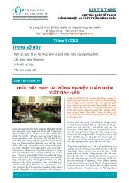
As the per capita income of countries increases, the contribution of the agricultural sector to
gross domestic product tends to decline. This structural transformation is seen clearly by comparing
the share of agriculture in low- and high-income countries (see Figure 2-1). Some of this shift is due
to urbanization and some to the growing importance of non-farm income sources in rural areas,
though the patterns vary across countries. Numerous studies of income and crop diversification have
Page 12

Chapter 2. Background on the Northern Uplands region
been carried out, although they are sometimes difficult to compare due to differences in the definition
of diversification. A selective review of some of these studies illustrates many of the points made in
Sections 2.1.2 and 2.1.3 of this chapter.
Figure 2-1. Structural transformation across countries
80
Share of agriculture in GDP (%)
70
60
Laos
50
40
30
Vietnam
20
10
Thailand
Japan
0
100 1,000 10,000 100,000
Per capita income (US$)
Source: World Bank, 2003.
Joshi et al (2002) examine the trends in diversification in South Asia using area and
production statistics and the Simpson Index of Diversity (SID). The SID is a measure of the number
of income sources and the balance among them (see Section 2.2.3 for more information). They show
that the diversity of crop production has increased over the past two decades in most South Asian
countries. In India, the southern and western regions are diversifying away from grains toward
pulses, oil seeds, fruits, and vegetables. In the northern region, farmers are turning from coarse grains
to commercial production of rice, wheat, and (to a lesser degree) non-grain crops. The eastern region
is poorer and less developed. Agriculture is dominated by rice, but the non-rice areas are quite
diverse. Carrying out state-level time-series econometric analysis, they show that diversification is
associated with road density, urbanization, average farm size, and per capita income. Rainfall is also
a significant factor: low-rainfall areas have more diverse cropping patterns than high-rainfall areas.
They conclude that diversification from coarse grains to high-yielding rice and wheat has had positive
effects on food security, while diversification toward cash crops has boosted employment per hectare
and agricultural exports.
Page 13

Chapter 2. Background on the Northern Uplands region
Reardon (1997) summarizes the results of 27 studies of rural non-farm employment in sub-
Saharan Africa. He finds that non-farm activities are relatively important in rural areas, accounting
for 30-50 percent of income in many cases. In general, non-farm wage labor is more important than
non-farm self-employment. Non-farm rural income tends to be more important in areas near cities
with good infrastructure and high population density. Finally, non-farm income is more important
among better-off rural households.
In a study of rural households in Ethiopia, Block and Webb (2001) find that diversification
out of crop production is associated with higher-income households, a higher dependency ratio, maleheaded
households, and location in the highlands (a region endowed with good soils and higher
rainfall). One of the motivations for diversifying out of crops, often into livestock activities, is to
provide insurance against drought. According to a survey, farmers believe that households with large
herds are less vulnerable to drought.
Delgado and Siamwalla (1997) examine patterns of income diversification in Asia and Africa.
They note that African farmers often have highly diversified crop mixes as a strategy to reduce risks
associated with bad weather. In many Asian countries, crop diversification is associated with
reducing the importance of rice and moving toward fruits, vegetables, and livestock activities. This
type of diversification raises income but exposes farmers to market risks, particularly when the
commodity is perishable. They argue that governments can play a constructive role in facilitating
institutions, such as cooperatives and contract farming, that facilitate diversification into high-value
commodities, thus raising rural income.
Liquidity constraints are often an important factor in the ability of households to diversify
into more remunerative activities. In Cote d’Ivoire, the 1994 currency devaluation increased the
incentives to grow cocoa, cotton, and other export crops, but richer households were better able to
take advantage of these opportunities, presumably due to greater liquidity. In Kenya, a food-for-work
program increased the liquidity of poor farmers, allowing them to diversify into non-crop activities
and avoid destocking livestock in drought years (Barrett et al, 2001).
Another study compares diversification in Rwanda, Kenya, and Cote d’Ivoire. Diversification
away from crop production is greatest in areas with low rainfall and poor soils. Although unskilled
labor income is associated with poor households, most other forms of non-farm income are positively
correlated with income. The fact that income diversity is greater among higher-income households
contradicts the idea that diversification is a risk management strategy (since we would expect the poor
to be more risk averse). On the other hand, it suggests that non-farm activities involve some barriers
to entry, such as education or capital, that make it difficult for poor households to participate (Barrett
et al, 2000b).
In Peru, non-farm activities make up roughly half of all rural income, though the percentage
varies widely across regions and households. The share of income from non-farm enterprises is
Page 14

Chapter 2. Background on the Northern Uplands region
positively correlated with education, electrification, proximity to market, and the value of crop output
per hectare (Escobal, 2001).
One study estimates the relationship between income diversification and household welfare in
Zimbabwe. Using household surveys carried out in 1990-91 and 1995-96, the study measured income
diversification by the number of income sources, the share of non-farm income, and the Simpson
index of diversity. The author finds that in rural areas, richer households had more diversified income
sources, while in urban areas the reverse was true (Ersado, 2003).
A recent study of West Punjab (India) looked at long-term trends in agricultural production
over the 20 th century (Kurosaki, 2003). This study found that area increase accounted for 71 percent
of the growth in an index of agricultural output 2 over 1903-1952, but in the period 1952-1992 the
most important contributors were yield increases (53 percent) and diversification (7 percent), where
diversification was defined as the reallocation of land toward higher-yielding crops. In the first
period, rice yield growth was due to concentration of rice production in the districts with higher and
growing yields, while in the second period, it was due to higher yields in each district. Finally,
analysis across districts indicates that road density is associated with diversification in the first period
and with specialization in the second period (Kurosaki, 2003).
Several studies have looked at the patterns of diversification in Vietnam. Pederson and
Annou (1999) examine the patterns of diversification using the 1992-93 Vietnam Living Standards
Survey. They find that agricultural diversification (defined as the share of non-rice output in
agricultural output) is associated with small farms, small irrigated areas, and higher levels of
education. In addition, they find that households whose crop production is relatively specialized in
rice tend to have more non-farm income diversification. This may suggest that household prefer some
form of diversification, either in non-rice production or in non-farm activities.
Henin (2002) provides a description of diversification patterns in the Northern Uplands,
focusing on Lang Son province. He argues that doi moi policies have increased income and
stimulated income diversification. Farmers in the study area have adopted modern rice varieties and
fertilizer (though they continue to use local varieties as well) and have expanded production of cash
crops such as sugarcane, peanuts, soybeans, tobacco, cinnamon, tea, and anis. Non-agricultural
activities are limited by the lack of rural industries, but some households earn income from porter
work, collecting firewood, bicycle and motorbike repair, and so on. Farmers identify a number of
constraints to diversification and poverty reduction: lack of capital, shortage of paddy land, poor
access to markets, poor irrigation infrastructure, and low quality education. Borrowing from the
formal sector, even from the concessionary Hunger Alleviation and Poverty Reduction Fund, is not
popular due to the high interest rates, short maturity of the loans, and complex procedures. Many
2
Because price data were not available throughout the 89-year period of the study, the author
constructed an index that combines production data on 12 major crops using fixed 1960 prices.
Page 15

Chapter 2. Background on the Northern Uplands region
farmers borrow informally from members of their kin network. Although the reforms have increased
income, they have also increased inequality, social differentiation, and a deterioration in some social
services.
A recent book contains a number of detailed studies of changes in land use and income
sources in Bac Kan Province (Castella and Dang Dinh Quang, 2002). Most of the studies provide a
long-term perspectives, describing changes in land-use patterns as a result of various changes in
policy and technology: collectivization in the late 1950s, the introduction of high-yielding rice
varieties in the late 1960s, the contract system under Decree 100 in 1981, decollectivization of land in
the years following Resolution 10 of 1988, and the Land Law of 1993, which began the process of
allocating land-use certificates. The studies use satellite imagery to document the progressive loss of
forest cover, particularly during the 1980s.
One study in Cho Moi District argues that the allocation of land has been successful in
stimulating intensification of lowland rice production, diversification in the uplands (particularly in
fruit), and preservation of forestland. Intensification of lowland production is not an alternative to
upland diversification; in fact, intensification has produced the liquidity and food security needed to
allow households to diversify on their upland plots (Fatoux et al, 2002).
A study of Ba Be District highlights the importance of accessibility in determining income
opportunities. In remote villages, farmers rely on subsistence crop and livestock production. They
have fewer opportunities to sell their output, speak with extension agents, benefit from government
programs, or obtain non-farm employment. As a result, they tend to be poorer than villages on main
roads close to urban centers, even if they have irrigated lowlands (Alther et al, 2002).
And a study in Cho Don District found that the ethnicity is becoming less useful as a predictor
of livelihood strategies. Historically, the Tay were sedentary lowland rice farmers, while the Dao
were nomadic and practiced shifting cultivation in upland areas. As a result of land allocations, land
purchases, and other factors, the distinction between Tay and Dao livelihood strategies is weak. Both
Tay and Dao farmers who have access to lowland paddy land are sedentary and grow irrigated rice,
while those without (both Tay and Dao) are forced to practice shifting cultivation (Castella et al,
2002).
Page 16

Chapter 2. Background on the Northern Uplands region
2.2 Background on the Northern Uplands
For the purpose of this report, we define the Northern Uplands to include the provinces in the
Northeast and Northwest regions 3 . This region is characterized by:
• Rugged upland terrain. Much of the Northern Uplands consists of hills and low
mountains between 500 and 1000 meters above sea level, but there are mountainous area
above 1000 meters (Nguyen Trong Dieu, 1995).
• Poor infrastructure. According to the 1994 Traffic Survey, the length of asphalted roads
in the Northern Upland region was 3271 kilometers, giving it a road density of 0.032
km/km 2 . By comparison, the national average is 0.045 km/km 2 (GSO, 1998: 779).
• Low population density. The population density in the Northern Uplands is 111
people/km 2 , which is low compared to the national figure of 231 people/km 2
• A large ethnic minority population. According to the data from the 1998 VLSS, 47
percent of the heads of household in the rural areas of the Northern Uplands belong to an
ethnic minority. In contrast, the figure for Vietnam as a whole is just 12 percent.
• Low levels of urbanization. According to GSO estimates for 2000, 16 percent of the
Northern Upland population lives in urban areas, compared to 23 percent nationally
(GSO, 2001).
• Importance of the agricultural sector. Agriculture, forestry, and fishing account for about
42 percent of the gross domestic product of the Northern Uplands region. For Vietnam as
a whole, this sector accounts for just 24 percent of GDP (GSO, 2001).
• A high incidence of poverty. According to the 1999 Vietnam Household Living
Standards Survey carried out by the General Statistical Office, the incidence of income
poverty in the Northeast and Northwest was 41 percent, higher than any other region,
though only slightly greater than in the North Central Coast and the Central Highlands
(GSO, 2000: 74). Similarly, the 1998 Vietnam Living Standards Survey estimated the
incidence of poverty in the Northern Uplands to be 59 percent, the highest of any region.
(Joint Working Group, 2000)
Behind these generalizations, however, a considerable amount of diversity exists within the
region. For example, across provinces, the population density varies from 36 to 395 people/km 2 , the
per capita gross domestic product (GDP) varies from less than VND 1.4 million to 3.7 million, and
the share of agriculture in GDP ranges from less than 10 percent to over 60 percent. Another
important point is that, although much of the region is poor, rural, and geographically isolated, this
does not imply that the rural economy is stagnant or that the region is being “left behind.” In fact, the
Northern Uplands is undergoing the same transformations (economic growth, urbanization,
3
The number of provinces in the Northern Uplands increased from 13 in 1995 (when it was called the
North Mountain and Midlands) to 16 in 1999 (when it was divided into two regions: the Northeast and
Northwest). Since 1999, two provinces (Vinh Phuc and Bac Ninh) have been reclassified as part of the Red
River Delta, leaving 14 provinces: eleven in the Northeast (Ha Giang, Cao Bang, Lao Cai, Bac Kan, Lang Son,
Tuyen Quang, Yen Bai, Thai Nguyen, Phu Tho, Bac Giang, and Quang Ninh) and three in the Northwest (Lai
Chau, Son La, and Hoa Binh).
Page 17

Chapter 2. Background on the Northern Uplands region
commercialization, poverty reduction, etc.) that are occurring elsewhere in Vietnam and in many
cases at the same rate. Thus, it is important to understand both the diversity within the region and the
trends over time. This chapter uses data from various sources to describe the geographic,
demographic, and economic diversity of the region. When possible, we present statistics for 1995 and
2000 to demonstrate the changes occurring in the region.
2.2.1 Geography
The Northern Uplands covers about 102 thousand square kilometers, representing a little less
than one third of the area of Vietnam. It is bordered by China on the north and the Lao P.D.R. to the
west and south. The region is bisected diagonally by the Red River (Song Hong) which runs from the
northwest to the southeast. Running parallel south of the Red River is the Black River (Song Da).
Much of the Northern Uplands consists of hills and low mountains with elevations between
500 and 1000 meters above sea level. The three provinces of the Northern Uplands to the west of the
Red River have large areas over 1000 meters, particularly in the Hoang Lien Son, a range than runs
between the Red River and the Black River. In fact, Fan Si Pan, the highest peak in Vietnam at 3143
meters above sea level, is in the province of Lao Cai in this range. The Northeast, the elevations are
not as high, but there are areas over 1000 meters. In Figure 2-2, the Red River valley can be seen as
a thin line entering Vietnam from the northwest, passing through Lai Chau, Yen Bai, and Phu Tho.
The rugged Hoan Lien Son mountain range is visible running parallel to the Red River to the south.
Figure 2-2 maps an index of accessibility based on the time it takes to get to the district
capital. The travel time is calculated using assumed fastest possible travel speed, taking into account
land cover, road quality, river navigability, the presence of bridges or ferries at the river-crossings,
and slope. The red and purple zones represent areas with less access (greater travel time to the district
headquarters). It is clear that Lai Chau is one of the least accessible provinces in the Northern
Uplands, followed by Son La and Lao Cai. Provinces in the Northeast generally have better
accessibility.
2.2.2 Population
As shown in Table 2-1, the region is home to 11.2 million people 4 , giving it a population
density of 111 people per square kilometer (km 2 ). As mentioned above, however, there is
considerable variation. Four provinces have more than 1 million inhabitants: Bac Giang, Phu Tho,
Thai Nguyen, and Quang Ninh. These four are also the most densely populated provinces in the
region with 173-395 people/km 2 . Three of the four are located on the edges of the Red River Delta,
with significant lowland areas and relatively good proximity to Hanoi. Quang Ninh is a special case
among these provinces because it is on the coast, allowing it to benefit from a large fishing sector, and
4
The figures given here are GSO estimates for the year 2000. The estimates are slightly higher than
the results of the 1999 Census which counted 11.1 million people in the 16 provinces considered here.
Page 18

Figure 2-2. Elevation of the Northern Upland region
Source: Elevation data from USGS GTOPO30, 2003.

Figure 2-3. Index of accessibility in the Northern Upland region
Source: Spatial analysis of GIS data from the Center for Remote Sensing & Geomatics.

Chapter 2. Background on the Northern Uplands region
Table 2-1. General indicators for the Northern Uplands by province in 1995 and 2000
Year
Population
Population
growth rate
Population
density
Agricultural
population
density
(rural
population/
hectare of
crop land)
Urban
population
GDP per
capita
(1000 1994
VND/
person)
Growth rate
in GDP per
capita
(1000
persons) (percent)
(population/
km 2 )
(percent)
(percent)
Ha Giang 1995 550.3 70 5.00 9% 945
2000 618.4 2.4% 78 4.67 11% 1,374 8%
Cao Bang 1995 489.2 73 4.99 10% 1,202
2000 497.4 0.3% 74 5.27 13% 2,171 13%
Lao Cai 1995 550.1 68 6.32 17% 1,366
2000 613.6 2.2% 76 5.85 17% 1,556 3%
Bac Kan 1995 254.2 52 8.16 13% 1,068
2000 280.7 2.0% 58 6.43 15% 1,461 6%
Lang Son 1995 679.2 82 7.22 17% 1,645
2000 710.7 0.9% 86 5.32 19% 2,436 8%
Tuyen Quang 1995 638.8 109 7.21 11% 1,379
2000 685.5 1.4% 117 6.85 9% 1,957 7%
Yen Bai 1995 647.7 94 7.24 19% 1,382
2000 691.6 1.3% 100 6.22 20% 1,938 7%
Thai Nguyen 1995 1,005.3 284 7.92 20% 1,662
2000 1,054.1 1.0% 298 6.22 21% 1,984 4%
Phu Tho 1995 1,211.7 344 8.96 10% 1,533
2000 1,273.5 1.0% 362 7.87 14% 2,184 7%
Bac Giang 1995 1431 374 6.67 6% 1,326
2000 1,509.3 1.1% 395 6.66 7% 1,771 6%
Quang Ninh 1995 941.7 160 7.50 43% 2,439
2000 1,017.7 1.6% 173 6.89 44% 3,708 9%
Lai Chau 1995 535.5 32 4.99 12% 1,440
2000 613.3 2.8% 36 5.12 12% 1,614 2%
Son La 1995 811.7 58 6.15 13% 884
2000 906.8 2.2% 65 5.05 11% 1,369 9%
Hoa Binh 1995 718.5 154 6.31 14% 1,255
2000 767.6 1.3% 165 5.77 14% 2,033 10%
Northern Uplands 1995 10,464.6 104 6.73 15% 1,446
2000 11,240.1 1.4% 111 6.06 16% 2,030 7%
Annual growth 1.4% 1.4% -2.09 1.4% 7.0%
Source: Calculations based on data from GSO (2001).
because it has large coal mining operations. At the other extreme, Bac Kan has the smallest
population (281 thousand) and Lai Chau, located in the far northwest bordering the Lao People’s
Democratic Republic and the People’s Republic of China, has the lowest population density: 36
people per square kilometer (see Table 2-1). The wide variation in population density is shown
graphically in Figure 2-4. In much of the Red River Delta, the density is over 1000 people/km 2 .
Outside the Delta, the population density falls off quickly to less than 200 people/km 2 .
The agricultural population density, defined as the rural population per hectare of crop land,
varies much less. Most provinces have between 5.0 and 7.0 rural inhabitants per hectare of crop land.
In addition, while population density of the Northern Uplands increased, the agricultural population
density has fallen due to the expansion of land under cultivation. Over 1995-2000, the population
growth rate for the region as a whole is estimated at 1.4 percent per year, though it differs widely
Page 21

Chapter 2. Background on the Northern Uplands region
across provinces. In general, the least densely populated provinces experience the highest growth
rates and vice versa. Lai Chau, the most sparsely populated province, has the highest rate of
population growth: 2.8 percent per year. Son La, Lao Cai, and Ha Giang, also with low densities, also
have growth rates of more than 2 percent. In contrast, the more densely populated provinces bordering
the Red River delta have growth rates in the range of 1-1.5 percent (see Table 2-1).
Overall, 16 percent of the people in the region lived in urban areas in 2000, up slightly from
15 percent in 1995. The degree of urbanization tends to range between 10 and 20 percent across
provinces. Quang Ninh is again an exception with the urban areas accounting for 44 percent of the
population. Bac Giang and Tuyen Quang have urbanization rates somewhat below 10 percent (see
Table 2-1).
Figure 2-5 shows the main ethnic group in each commune in northern Vietnam. Note that the
map indicates the most common ethnic group, but this group does not necessarily constitute a
majority of the population in that commune. The map shows that the Kinh (ethnic Vietnamese) are the
main group in the Delta region, as well as in most of Bac Giang, the southern half of Thai Nguyen, the
northern part of Phu Tho, and parts of Yen Bai. The Tay, the most numerous of the ethnic minorities,
live among the Nung in the valleys and plains of Bac Kan, northern Tuyen Quang, and parts of other
provinces in the Northeast. The Tay are more similar culturally and economically to the Kinh than
many minority groups. The Nung, the second most numerous minority, are concentrated in Lang Son
and Cao Bang. The Thai are the main ethnic group in much of Son La province and parts of Lai Chau.
The Muong are found in Hoa Binh and parts of Phu Tho and Son La. The Hmong (Meo) are more
spread out, being found in Son La, Lai Chau, Yen Bai, and northern Ha Giang, often living at higher
altitudes (above 1500 meters). The Dao live at middle altitudes (700-1000 m) are similarly scattered
(Nguyen Trong Dieu, 1995).
2.2.3 Land use and agriculture
Contribution of agriculture to GDP
One measure of the importance of the agricultural sector is its contribution to gross domestic
product (GDP). Agriculture (defined broadly to include crops. livestock, fishing, and forestry)
accounts for 24 percent of national GDP, but 42 percent of the GDP in the Northern Uplands. As
shown in Table 2-2, agriculture plays a particularly important role in the poorer, more remote border
provinces such as Ha Giang, Cao Bang, and Son La, where it represents over half of GDP.
Agriculture plays a somewhat smaller role in the higher-income interior provinces close to Hanoi such
as Thai Nguyen and Phu Tho, where it is 30-40 percent of the total. Quang Ninh is the most industrial
and the highest-income province in the region. Agriculture in Quang Ninh province accounts for just
9 percent of GDP, while industry and construction (including mining) represents almost half of GDP.
Page 22

Figure 2-4. Population density in the Northern Upland region
Source: Analysis of data from the 1999 Population and Housing Census.

Figure 2-5. Main ethnic group in each commune of the Northern Uplands
Source: Analysis of the 1999 Population and Housing Census.

Chapter 2. Background on the Northern Uplands region
Table 2-2. Structure of gross domestic product in the Northern Uplands
by province in 1995 and 2000
Agric
ulture, forestry,
Year & fishing
Industry &
construction Services Total
Ha Giang 1995 69% 15% 16% 100%
2000 54% 21% 25% 100%
Cao Bang 1995 73% 7% 19% 100%
2000 56% 16% 29% 100%
Lao Cai 1995 51% 22% 27% 100%
2000 48% 22% 30% 100%
Bac Kan 1995 71% 6% 23% 100%
2000 66% 9% 25% 100%
Lang Son 1995 62% 8% 30% 100%
2000 50% 11% 38% 100%
Tuyen Quang 1995 56% 16% 28% 100%
2000 52% 20% 29% 100%
Yen Bai 1995 52% 26% 22% 100%
2000 45% 28% 27% 100%
Thai Nguyen 1995 38% 33% 28% 100%
2000 39% 32% 29% 100%
Phu Tho 1995 36% 31% 33% 100%
2000 31% 37% 32% 100%
Bac Giang 1995 53% 17% 29% 100%
2000 55% 14% 31% 100%
Quang Ninh 1995 11% 38% 50% 100%
2000 9% 48% 43% 100%
Lai Chau 1995 49% 14% 37% 100%
2000 46% 18% 37% 100%
Son La 1995 73% 10% 17% 100%
2000 62% 10% 27% 100%
Hoa Binh 1995 60% 6% 33% 100%
2000 52% 17% 31% 100%
Northern Uplands 1995 47% 22% 31% 100%
2000 42% 26% 33% 100%
Change -5 +4 +2
Source: Calculations based on data from GSO (2001).
Land use
The figures presented in Table 2-3 indicate that only a 15 percent of the land area in the
region is under cultivation. Almost half (47 percent) of the total land area is classified as “unused
land”, which includes large tracts of land that is unusable either because the topography is too rugged,
because it is too remote, or because it has been degraded (the so-called “barren land”). Another 37
percent of the area is classified as forest land, although this category includes actual forests and areas
that are designated to be reclaimed as forest. The share of total land being used for cultivation is
lowest in Lai Chau (6 percent) and ranges from 11 to 15 percent in the other border provinces. The
interior province of Bac Giang is the only province in the region with more than 50 percent of the
total area devoted to crop production. Thai Nguyen and Phu Tho, two other provinces with lowland
areas, good access, and a high population density, have more than 35 percent of the land area in crops
(see Table 2-3).
Page 25

Chapter 2. Background on the Northern Uplands region
Table 2-3. Land resources and productivity in the Northern Uplands by province
in 1995 and 2000
Total land area Total cropped Cropped area as
Agricultural GDP
per hectare
Year
area percent of total
(1000 ha) (1000 ha) (percent)
(million 1994 VND
/cropped ha)
Ha Giang 1995 788 100.2 13% 3.60
2000 788 117.9 15% 3.87
Cao Bang 1995 669 88.2 13% 4.89
2000 669 82.1 12% 7.32
Lao Cai 1995 806 72.3 9% 5.28
2000 806 87.1 11% 5.31
Bac Kan 1995 486 27.1 6% 7.14
2000 486 37.1 8% 7.29
Lang Son 1995 830 78.1 9% 8.90
2000 830 108.3 13% 8.05
Tuyen Quang 1995 587 78.8 13% 6.25
2000 587 91.1 16% 7.60
Yen Bai 1995 688 72.5 11% 6.39
2000 688 88.9 13% 6.76
Thai Nguyen 1995 354 101.5 29% 6.33
2000 354 133.8 38% 6.03
Phu Tho 1995 352 121.7 35% 5.47
2000 352 139.2 40% 6.15
Bac Giang 1995 382 201.6 53% 5.04
2000 382 210.9 55% 6.99
Quang Ninh 1995 590 71.6 12% 3.67
2000 590 82.7 14% 4.27
Lai Chau 1995 1692 94.5 6% 3.97
2000 1692 105.4 6% 4.29
Son La 1995 1405 114.9 8% 4.56
2000 1405 159.7 11% 4.86
Hoa Binh 1995 466 98 21% 5.55
2000 466 114.4 25% 7.07
Northern Uplands 1995 10096 1321.0 13% 5.33
2000 10096 1558.6 15% 6.08
Annual growth 0.0% 3.4% 2.7%
Source: Calculations based on data from GSO (2001).
The last column in Table 2-3 shows the value of agricultural output per hectare of crop land.
This is one measure of crop diversification because as household diversify from low-value staple
crops to higher-value commercial crops, this is reflected in rising value per hectare. On average,
cropland in the Northern Uplands produces VND 6.1 million per hectare (in constant 1994 prices).
The provincial figures reveal two patterns. First, the value per hectare is generally greater in the
interior provinces close to Hanoi than in the remote border provinces. For example. Ha Giang, Lai
Chau, and Son La have values of less than VND 5 million per hectare of cropland. And the interior
provinces of Tuyen Quang, Yen Bai, Phu Tho, Bac Giang, Hoa Binh, and Thai Nguyen have
agricultural output worth more than VND 6 million per hectare. There are some exceptions to this
pattern, notably the high values found in Lang Son and Cao Bang. In the case of Lang Son, part of
the explanation lies in the large forestry sector, which is included in the broad definition of
Page 26

Chapter 2. Background on the Northern Uplands region
agriculture. In addition, Lang Son is the main gateway for exports to China, giving the province an
advantage in producing for export.
The second pattern that is evident is that the value of agricultural output per hectare increased
substantially, rising from VND 5.3 million/ha in 1995 to VND 6.1 million/ha in 2000. This represents
an increase of 2.2 percent per year. Although this increase is consistent with crop diversification, in
which farmers shift from low-value to high-value crops, it may also reflect higher yields and/or higher
crop prices. Thus, it is useful to examine the allocation of cropland among different crops.
Agricultural data from the General Statistics Office suggest that rice remains the dominant
crop in the Northern Uplands, but that the share of cropland allocated to rice is declining. As shown
in Table 2-4, sown rice area 5 has fallen from 50 percent of the total to 44 percent. Furthermore, this
decline can be observed in every province except one (Bac Giang). In Bac Kan and Son La, the
percentage of cropland planted with rice declined dramatically, falling by more than 10 percentage
points over the five-year period. Other food crops (maize, cassava, and sweet potatoes) show no net
change for the region as a whole, but this masks some variation across provinces. Most provinces
experienced a small decrease in the share of area allocated to non-rice food crops, but this was offset
by large increases in Son La and Bac Kan. In Son La, maize production has grown strongly in recent
years to supply the feed industry which in turn has been stimulated by the growth of urban demand for
poultry and pork.
The share of cropland allocated to vegetables and beans increased slightly, as did the share of
area devoted to tea and coffee (of which tea represents 93 percent), while the share allocated to annual
industrial crops fell slightly. But the most noteworthy trend is the growth in the share of cropland
devoted to “other crops,” which has increased from 6 percent in 1995 to 11 percent in 2000. The
largest increase is in the province of Lang Son, on the northern border with China. The category
“other crops” presumably includes fruit trees, other tree crops, and agro-forestry plantations. The
growth in litchi and longan production for domestic consumption and for export to China probably
accounts for the main part of this increase. It should be noted, however, that we have calculated
“other crops” as a residual of total crop area after subtracting the other crop categories.
Crop production
The falling share of cropland allocated to rice cultivation raises questions about the impact of
crop diversification on food security. Are farmers in the Northern Uplands sacrificing food security
in pursuit of higher profits from vegetables, tea, and fruit The question is particularly relevant in
light of the fact that the rural Northern Uplands is the poorest region of Vietnam so food security is
clearly an important issue. Table 2-5 shows that the amount of rice land in the Northern Uplands has
5 “Sown area” adds the areas planted in different seasons, so that one hectare of double-cropped rice is
counted as two hectares.
Page 27

Chapter 2. Background on the Northern Uplands region
remained virtually unchanged over the period 1995-2000. Furthermore, a crude measure 6 of rice
cropping intensity suggests that it has increased only slightly, rising from 1.47 to 1.51 over the fiveyear
period.
Table 2-4. Allocation of cropped area in the Northern Uplands by province in 1995 and 2000
Year
Rice
Other food
crops
Percentage of cropped area
Annual
industrial
crops
Vegetables
& beans
Coffee
& tea
Other
crops
---------------------------------------------(percent)--------------------------------------------
Ha Giang 1995 29% 44% 8% 6% 7% 6% 100%
2000 26% 39% 9% 8% 8% 9% 100%
Cao Bang 1995 38% 43% 3% 12% 0% 4% 100%
2000 35% 43% 5% 14% 0% 4% 100%
Lao Cai 1995 46% 35% 8% 8% 2% 1% 100%
2000 42% 34% 4% 9% 2% 9% 100%
Bac Kan 1995 66% 19% 4% 7% 1% 3% 100%
2000 50% 34% 4% 6% 1% 6% 100%
Lang Son 1995 58% 21% 6% 9% 1% 5% 100%
2000 43% 18% 5% 6% 1% 27% 100%
Tuyen Quang 1995 51% 23% 4% 13% 5% 3% 100%
2000 49% 22% 5% 14% 4% 7% 100%
Yen Bai 1995 53% 21% 6% 4% 10% 7% 100%
2000 45% 24% 6% 4% 12% 10% 100%
Thai Nguyen 1995 58% 18% 7% 9% 8% 0% 100%
2000 51% 20% 6% 8% 9% 6% 100%
Phu Tho 1995 58% 19% 7% 6% 6% 4% 100%
2000 51% 21% 7% 7% 6% 8% 100%
Bac Giang 1995 54% 18% 6% 8% 0% 13% 100%
2000 55% 14% 8% 6% 0% 17% 100%
Quang Ninh 1995 63% 18% 9% 8% 0% 3% 100%
2000 59% 16% 9% 5% 0% 11% 100%
Lai Chau 1995 50% 38% 2% 6% 1% 3% 100%
2000 49% 38% 3% 6% 2% 2% 100%
Son La 1995 38% 34% 2% 12% 3% 11% 100%
2000 26% 43% 3% 10% 4% 14% 100%
Hoa Binh 1995 44% 28% 3% 13% 3% 9% 100%
2000 38% 32% 5% 11% 2% 12% 100%
Northern Uplands 1995 50% 27% 5% 9% 3% 6% 100%
2000 44% 27% 6% 8% 4% 11% 100%
Change -6 0 +1 -1 +1 +5
Source: Calculations based on data from GSO (2001).
Total
Combining the changes in rice land and cropping intensity, the sown area of rice increased less than 1
percent per year over the period 1995-2000. Paddy yields, however, have increased from 2.7 tons/ha
in 1995 to 3.6 tons/ha in 2000, equivalent to an annual growth rate of almost 6 percent. The
combined effect of the small increase in sown area and the large increase in yield is that rice produc-
6
Rice cropping intensity is calculated as the sum of sown rice area divided by the area planted with
rice in any season. In the absence of data on the latter, we approximate rice intensity as the sum of spring and
winter area divided by larger of the two figures. This represents an upper limit on the true rice cropping
intensity.
Page 28

Chapter 2. Background on the Northern Uplands region
Table 2-5. Cereal production in the Northern Uplands by province in 1995 and 2000
Rice Rice area
Rice
cropping
Paddy Rice output Maize
Maize
output per
Year land sown intensity Paddy yield output per capita output capita
(kg/ (1000 (kg/
(1000 ha) (1000 ha) (ratio) (tons/ha)(1000 tons) person) tons person)
Ha Giang 1995 23.5 29.3 1.25 2.80 81.9 98 45.4 83
2000 23.7 31.2 1.32 3.88 121.0 129 71.3 115
Cao Bang 1995 30.1 33.4 1.11 2.77 92.4 125 55.3 113
2000 25.2 28.6 1.13 3.10 88.8 118 75.8 152
Lao Cai 1995 26.4 33.1 1.25 2.49 82.5 99 27.7 50
2000 27.7 36.4 1.31 3.07 111.7 120 38.3 62
Bac Kan 1995 14.4 18.0 1.25 2.81 50.5 131 5.1 20
2000 13.3 18.6 1.40 3.67 68.3 161 20.3 72
Lang Son 1995 34.6 45.4 1.31 2.83 128.5 125 21.6 32
2000 33.9 46.9 1.38 3.09 145.0 135 42.8 60
Tuyen Quang 1995 26.4 40.3 1.53 3.32 133.7 138 24.8 39
2000 26.6 44.5 1.67 4.47 198.9 192 36.6 53
Yen Bai 1995 24.3 38.5 1.58 3.14 120.7 123 9.4 15
2000 24.8 39.9 1.61 3.77 150.5 144 19.5 28
Thai Nguyen 1995 37.6 59.2 1.57 3.03 179.4 118 10.1 10
2000 42.7 68.6 1.61 3.89 267.1 167 30.6 29
Phu Tho 1995 35.9 70.2 1.96 2.62 183.6 100 23.9 20
2000 36.3 71.6 1.97 4.04 289.1 150 42.2 33
Bac Giang 1995 60.4 109.8 1.82 2.62 287.7 133 13.9 10
2000 64.3 115.0 1.79 4.14 475.6 208 28.9 19
Quang Ninh 1995 28.0 45.1 1.61 2.59 116.7 82 6.0 6
2000 30.1 48.4 1.61 3.64 176.0 114 12.9 13
Lai Chau 1995 41.9 47.4 1.13 2.13 100.8 124 30.1 56
2000 45.2 51.9 1.15 2.52 130.7 141 41.0 67
Son La 1995 37.7 43.6 1.16 2.28 99.4 81 45.6 56
2000 34.8 41.5 1.19 2.49 103.3 75 122.1 135
Hoa Binh 1995 27.1 43.5 1.61 2.96 128.7 118 20.6 29
2000 26.9 43.4 1.61 3.73 161.9 139 48.7 63
Northern Uplands 1995 446.7 656.8 1.47 2.72 1,786.5 113 339.5 32
2000 454.5 686.5 1.51 3.62 2,487.9 146 631.0 56
Annual growth 0.3% 0.9% 0.5% 5.9% 6.8% 5.3% 13.2% 11.6%
Source: Calculations based on data from GSO (2001).
tion in the Northern Uplands has grown 6.8 percent per year. Per capita rice production has grown
from 113 kg/person to 146 kg/person, a growth rate of more than 5 percent annually. Thus, farmers
are not sacrificing rice production to diversify into higher-value crops. Instead, they are moving
slowly toward rice self-sufficiency on the basis of higher yields, while allocating any new land to
higher-value crops such as vegetables, fruit, and tea.
Maize output has grown even more rapidly, rising 13 percent annually. Son La maize
production has increased more than 160 percent over the five-year period, making it the main maize
producer in the region. As mentioned earlier, the growing demand for animal feed by poultry and pig
producers s driving the demand for maize.
Page 29

Chapter 2. Background on the Northern Uplands region
2.2.4 Income and poverty
The per capita gross domestic product of the region is VND 2.0 million (expressed in 1994
prices). The per capita GDP ranges from below VND 1.4 million in Ha Giang and Son La to VND
3.7 million in Quang Ninh. After Quang Ninh, no other province has a per capita GDP over VND
2.5 million. Between 1995 and 2000, per capita GDP in the region has grown 7 percent per year. The
slowest growing provinces over this period were Lao Cai and Lai Chau, whose economies grew at 2-3
percent per year in per capita terms. Since these are some of the most remote regions, one might
assume that there is a relationship between proximity to Hanoi and the growth rate. In fact, the
relationship is not very clear. The fastest growing province in the region is Cao Bang, on the northern
border with China and other border-provinces such as Ha Giang and Son La registered growth rates
above the regional average (see Table 2.6).
The incidences of poverty at the district level was estimated by combining data from the 1998 VLSS
and the 1999 Population and Housing Census. The VLSS data were used to estimate econometrically
the relationship between per capita expenditure and various household characteristics including size
and composition of the household, housing characteristics, ownership of consumer durables, type of
water source, type of toilet, and region. This relationship is then applied to the same household
characteristics taken from the 1999 Census (see by Minot and Baulch, 2002 for more details). The
results indicate that poverty is more widespread in the more remote districts, particularly those along
the Lao and Chinese border. Closer to Hanoi and to the Red River Delta, the incidence of poverty is
lower (see Figure 2-6). Using this method, the estimated national poverty rate from the Census data
was 36.5 percent, compared to 37.4 percent as estimated directly from the 1998 VLSS. By contrast,
the poverty rate in the rural Northern Uplands was 60 percent (see Table 2-6). The highest incidences
of rural poverty were found in Lai Chau, Son La, Ha Giang, Lao Cai, and Cao Bang. These five
provinces are not just the poorest in the Northern Uplands, but according to this analysis, they are the
poorest five provinces in the country. 7 The least poor rural areas in the Northern Uplands are those of
Phu Tho, Bac Giang, and Thai Nguyen. These correspond to the provinces closes to Hanoi and
adjacent to the Red River Delta.
7 The 95 percent confidence interval of these estimates is ± 6-8 percent, so we cannot say with
confidence that, for example, the rural areas of Lai Chau are poorer than those of Son La.
Page 30

Figure 2-6. Estimates of the incidence of poverty at the district level
Source: Analysis of the 1999 Population and Housing Census and the 1998 VLSS.

Chapter 2. Background on the Northern Uplands region
Table 2-6. GDP per capita and estimated poverty
GDP per capita
Annual growth
rate in GDP per
capita
Estimated
incidence of
poverty
1995 2000 1995-2000 1999
(1000 1994 VND/person) (percent) (percent)
Ha Giang 945 1,374 8% 77%
Cao Bang 1,202 2,171 13% 74%
Lao Cai 1,366 1,556 3% 75%
Bac Kan 1,068 1,461 6% 68%
Lang Son 1,645 2,436 8% 72%
Tuyen Quang 1,379 1,957 7% 63%
Yen Bai 1,382 1,938 7% 64%
Thai Nguyen 1,662 1,984 4% 49%
Phu Tho 1,533 2,184 7% 48%
Bac Giang 1,326 1,771 6% 49%
Quang Ninh 2,439 3,708 9% 52%
Lai Chau 1,440 1,614 2% 86%
Son La 884 1,369 9% 79%
Hoa Binh 1,255 2,033 10% 65%
Northern Uplands 1,446 2,030 7.0% 60%
Source: GDP figures from GSO (2001).
Poverty estimates from Minot and Baulch (2002).
2.2.5 Income diversification
Three measures of income diversification can be calculated from the GSO data. The first
measure of diversification is the share of GDP generated outside the agricultural sector (defined
broadly to include crops, livestock, fishing, and forestry). Overall, the non-agricultural share of GDP
has increased from 53 to 58 percent. The increase is largest for Cao Bang (17 percentage point
increase), Ha Giang (15 percentage points), Lang Son (12 percentage points) and Son La (11
percentage points). The increase is quite small in Quang Ninh (from 89 to 91 percent), partly
because the non-agricultural sector is already so dominant. And in Bac Giang and Thai Nguyen, the
share of non-agricultural sector actually declined slightly. These are the only provinces that experienced
this type of change (see Table 2-7 and Figure 2-7). Figure 2-8 plots the changes in the contribution of
agriculture to GDP against changes in GDP per capita. Provinces with higher income tend to have a
smaller agricultural component, but almost all provinces show both economic growth and declining
share of agriculture. This process is known as the structural transformation of the economy.
The second measure is the share of cultivated land in crops other than rice. Overall, the share
of non-rice crops has increased from 50 percent in 1995 to 56 percent in 2000. As mentioned earlier,
the share of non-rice crops expanded in every province except one (Bac Giang), with the largest shifts
occurring in Bac Kan, Lang Son and Son La (see Table 2-7).
Page 32

Chapter 2. Background on the Northern Uplands region
The third measure of crop diversification is the share of cropland allocated to non-food
crops 8 . Under this definition, unlike the previous one, a shift from rice to maize would not be
considered crop diversification. Overall, the share of cropland planted with non-food crops grew
from 23 percent to 28 percent. The largest increase was found in Lang Son, where it increased from
21 percent to 39 percent, presumably in response to trade with China (see Table 2-7 and Figure 2-9).
Table 2-7. Measure of income diversification in the Northern Uplands
by province in 1995 and 2000
Non-agricultural Non-rice area as Non-food area as
Year
GDP as
percentage of total
percentage of
crop area
percentage of
crop area
Ha Giang 1995 31% 71% 27%
2000 46% 74% 34%
Cao Bang 1995 27% 62% 19%
2000 44% 65% 22%
Lao Cai 1995 49% 54% 20%
2000 52% 58% 24%
Bac Kan 1995 29% 34% 15%
2000 34% 50% 16%
Lang Son 1995 38% 42% 21%
2000 50% 57% 39%
Tuyen Quang 1995 44% 49% 25%
2000 48% 51% 29%
Yen Bai 1995 48% 47% 26%
2000 55% 55% 31%
Thai Nguyen 1995 62% 42% 24%
2000 61% 49% 29%
Phu Tho 1995 64% 42% 23%
2000 69% 49% 27%
Bac Giang 1995 47% 46% 27%
2000 45% 45% 32%
Quang Ninh 1995 89% 37% 19%
2000 91% 41% 26%
Lai Chau 1995 51% 50% 12%
2000 54% 51% 12%
Son La 1995 27% 62% 28%
2000 38% 74% 31%
Hoa Binh 1995 40% 56% 27%
2000 48% 62% 30%
Northern Uplands 1995 53% 50% 23%
2000 58% 56% 28%
Change +5 +6 +5
Source: Calculations based on data from GSO (2001).
8 Food crops are defined as rice, maize, sweet potatoes, and cassava
Page 33

Figure 2-7. Diversification into non-agricultural activities over 1995-2000
Source: Calculations based on data from GSO (2001).

Figure 2-8. Structural transformation of the provinces of the Northern Uplands
80%
1995
70%
Agriculture as % of GDP
60%
50%
40%
30%
20%
10%
Ha Giang
Cao Bang
Lao Cai
Bac Kan
Lang Son
Tuyen Quang
Yen Bai
Thai Nguyen
Phu Tho
Bac Giang
Lai Chau
Son La
Hoa Binh
2000
0%
0 500 1000 1500 2000 2500 3000
GDP per capita (1000 VND)
Source: Calculations based on data from GSO (2001)

Figure 2-9. Diversification into non-food crops over 1995-2000
Source: Calculations based on data from GSO (2001).

Chapter 2. Background on the Northern Uplands region
2.3 Summary
Diversification has been defined in various ways. Some studies define it as an increase in the
number of income-generating activities or the balance among them. Others focus on the transition
from subsistence agriculture to commercial production. And a third definition emphasizes the
reallocation of resources from crops with low returns (typically staple food crops) to crops and
activities with higher returns.
Rural households adopt multiple income sources to manage risk, take advantage of
externalities, adapt to missing markets, respond to heterogeneous skills in the household, or meet
diverse consumption needs. Diversification into high-value activities is often inhibited by barriers to
entry. These include lack of liquidity for investment, lack of information about production and
marketing, lack of education or language skills, lack of social capital, and poor infrastructure.
Although income and crop diversification is usually considered a positive trend, some
concerns have been raised about its impact on food security and nutrition, regarding the consequences
for income inequality and social differentiation, and about its environmental sustainability. Empirical
research on diversification show different patterns by region. There is evidence that crop
diversification is greater among poor households in less favored agro-ecological zones, while nonfarm
income diversification is associated with higher income, more education, and proximity to large
markets.
Turning our attention to the Northern Uplands, the topography is hilly to mountainous, with
altitudes typically between 500 and 1000 meters but with some mountainous areas with peaks above
3000 meters. The infrastructure is poor, leading to communities being relatively isolated from the rest
of the economy. Roughly 11 million people live in the region, resulting in a population density that is
low (111 people/km 2 ) compared to the country as a whole (231 people/km 2 ). Roughly half the
population is a member of an ethnic minority, compared to just 12 percent nationally. The region is
less urbanized and more dependent on the agricultural sector than other regions of Vietnam. And the
incidence of poverty is probably highest in the Northern Uplands, though some studies rank the North
Central Coast and the Central Highlands as equally poor.
Nonetheless, there is considerable diversify across the Northern Uplands. The topography is
highest and most rugged in Lai Chau, Lao Cai, and Son La, while provinces adjacent to the Red River
Delta have significant lowland areas. The infrastructure is better and the population density is much
higher in the provinces near the Delta such as Thai Nguyen, Bac Giang, and Phu Tho. Although
ethnic minorities dominate in most of the Northern Uplands, Kinh are the main ethnic group in large
areas of Thai Nguyen, Bac Giang, Phu Tho, and Quang Ninh. The level of urbanization varies from 7
percent in Bac Giang to 44 percent in Quang Ninh,. Similarly, the incidence of poverty varies widely,
being greatest in the border provinces such as Lai Chau, Ha Giang, and Son La and lowest in Quang
Ninh and provinces adjacent to the Delta.
Page 37

Chapter 2. Background on the Northern Uplands region
Some general trends in the Northern Uplands can be identified by comparing statistics for
1995 and 2000. Although the agricultural sector is growing rapidly (6 percent per year), the
agricultural share of GDP has fallen from 47 percent to 42 percent over this period, indicating that
non-agricultural diversification is occurring at the regional level. The area allocated to rice has been
almost unchanged over this period, but rice production per capita has grown significantly due to rising
yields and, to a lesser extent, cropping intensification. At the same time, there is evidence of crop
diversification in that the share of crop land allocated to non-rice crops and non-food crops has
increased by 5-6 percentage points. Finally, the growth in agricultural GDP per hectare suggests a
trend of diversification into higher-value crops and other agricultural activities. These trends, and
their impact on living standards, are discussed in the next chapter.
Page 38

CHAPTER THREE
PATTERNS AND TRENDS IN DIVERSIFICATION:
ANALYSIS OF THREE NATIONAL HOUSEHOLD SURVEYS
3.1 Introduction
Between 1993 and 1998, rural poverty fell from 66 percent to 45 percent (Joint Government-
World Bank-NGO Working Group, 2000). Part of the reduction in poverty is due to higher yields of
rice and other crops, which have allowed Vietnam to become the second largest rice exporter with no
expansion in rice area and no reduction in domestic consumption (Minot and Goletti, 2000). In
addition, Vietnamese farmers have diversified into higher-value crops. Vietnam has become the
second largest coffee producer in the world, and production and export of fruits and vegetables have
risen dramatically over this period. And part of the income growth and poverty reduction is
undoubtedly due to diversification into non-crop activities such as aquaculture, livestock raising, and
non-farm activities.
The importance of each of these factors in rural income growth and poverty reduction has
implications for policy and public investment. If most income growth comes from technological
change which increases yields, then investments in agricultural research deserve priority 1 . If income
growth derives largely from crop diversification, then research into the constraint that prevent some
farmers from diversifying deserves greater attention. And if income growth or poverty rises mostly
due to the switch to non-farm activities, then non-farm employment generation should be the focus of
research.
Furthermore, the most important factor in raising rural incomes may be different than the
most important factor in reducing rural poverty. For example, it may be that low-income households
benefit more from higher yields and crop diversification, while higher-income households gain with
diversification into non-farm activities. The latter effect could dominate the increase in average rural
income, while the former would have a larger impact on the incidence of poverty.
Finally, it is possible that the importance of each factor will vary depending on household
characteristics and location. For example, yield increases may be more important for farmers in
irrigated lowland areas, crop diversification may be important to household near roads and market
infrastructure, and diversification into non-farm activities to be important near urban areas.
In light of the rapid growth in rural income in Vietnam and the lack of information on the
sources of growth, this study will focus on the following questions:
1
In theory, investment decisions should be made based on the size of the marginal contribution to
growth from alternative investments. However, since this information is generally not available, a reasonable
approximation is to allocate investment among growth strategies according to the average contribution to
economic growth.
Page 39

Chapter 3. Patterns and trends in diversification
• What is the relative importance of various sources of rural income growth in Vietnam:
yield increases, crop price increases, diversification into high-value crops, growth in
livestock and aquaculture, or the shift toward non-farm activities.
• What is the relative importance of these factors in the dramatic reduction in rural poverty
in Vietnam
• How do the sources of income growth and poverty reduction vary by region and by type
of household
3.2 Data and methods
What is income diversification and how do we measure it Before analyzing the patterns and
trends in income diversification in the north mountain region of Vietnam, it is important to address
these two questions. In this section, we briefly describe the data used in this section, the definitions of
diversification adopted, and the measures of diversification used.
3.2.1 Data
This report uses three national household surveys to examine the patterns and trends in
income diversification. The first Vietnam Living Standards Survey (VLSS) was carried out in 1992-
93 by the State Planning Committee and the General Statistics Office, with financial contributions
from the United Nations Development Programme (UNDP) and the Swedish International
Development Agency (SIDA) and technical assistance from the World Bank. The survey included a
household survey, a community survey, and a market price survey. The household survey covered
household size and composition, health, anthropometric measures of nutrition, education, housing
characteristics, migration, employment, non-farm enterprises, agriculture, other income, expenditure
and food consumption, ownership of consumer durables, and savings and credit. The household
questionnaire was approximately 110 pages long and included about 1000 questions. The sample was
selected in three stages using data from the 1989 Population Census. First, 120 villages and 30 urban
precincts were selected at random, with probabilities proportional to the population. Then two rural
hamlets or urban blocks were selected in each selected village/precinct. Finally, 16 households were
selected in each selected hamlet/block, making a total sample of 4800 households (see SPC/GSO,
1994 for more details). The sample was designed to be representative at the level of the seven
geographic regions of Vietnam. The survey was implemented between October 1992 and October
1993. Because the bulk of the data collection took place in 1993, we will refer to it as the 1993 VLSS.
The second Vietnam Living Standards Survey was conducted in 1997-98 by the General
Statistics Office, with financial support from the UNDP and SIDA and technical assistance from the
World Bank. Like the 1993 VLSS, the survey included a household survey, a community survey, and
a market price survey, though a survey of health centers was added. The household questionnaire
covers the same topics as the 1993 VLSS, with only slight changes in the questions and format. The
household sample includes most of the households from the 1993 VLSS, as well as additional
Page 40

Chapter 3. Patterns and trends in diversification
households to provide better coverage of urban areas and the Central Highlands 2 . The sample
contains 6000 households and is representative for each of ten strata, the rural areas of the seven
geographic regions and three urban strata (Hanoi and Ho Chi Minh City, other cities, and towns). The
data collection began in December 1997 and was completed in December 1998. We will refer to this
survey as the 1998 VLSS.
The Vietnam Household Living Standards Survey (VHLSS) was carried out in 2002 by the
General Statistics Office with support from the United Nations Development Programme, the Swedish
International Development Agency, the Japan Bank for International Cooperation and the World
Bank. The VHLSS has two versions: a small questionnaire (36 pages) administered to about 45,000
households and a larger questionnaire (43 pages) administered to a smaller sample of about 30,000.
The larger questionnaire has an expenditure module, allowing calculation of more reliable
expenditure-based estimates of living standards. In this analysis, we use the data from the first two
rounds of the smaller-sample version because we need expenditure data for comparability with the
two VLSS surveys. The larger VHLSS questionnaire is similar to the VLSS questionnaire except that
some modules are not included (anthropometrics, migration, and savings and credit) and most of the
other modules are simplified. For example, the VHLSS does not collect crop-level information on
seed, fertilizer, and other input costs, so it is not possible to calculate net income from each crop.
Table 3-1.summarizes the differences across the three surveys.
Table 3-1. Characteristics of the household surveys
Name
Period of
data
collection
Sample
size
Length of the
household
questionnaire
1993 Vietnam
Living Standards
Survey
1998 Vietnam
Living Standards
Survey
2002 Vietnam
Household
Living Standards
Survey
1992-
1993
1997-
1998
2002
Lowest level of
representativeness
Types of data collected
4800 110 pages Seven regions Household member characteristics,
education, health, employment,
migration, housing, fertility,
agriculture, non-farm selfemployment,
expenditure, assets, other
income, and savings and credit.
6000 110 pages Ten strata (7 rural
regions and 3 types
of urban areas)
30,000 43 pages Urban and rural
areas of eight
regions
Almost identical content and structure
as the 1992-93 VLSS.
Similar to VLSS but no migration,
anthropometrics, savings, or credit
modules. Other modules simplified
45,000 36 pages 61 provinces Similar to small-sample VHLSS but no
expenditure module.
3.2.2 Calculation of income
Income is calculated from both the VLSS and the VHLSS as the sum of net revenues from the
following sources: crop production, agricultural by-products, livestock production, aquaculture,
2
Because the 1993 VLSS sample was designed to be proportional to the population, the sample for
the sparsely populated Central Highlands was just 128 households. In the 1998 VLSS, two clusters from the
1993 VLSS sample in the Red River Delta were dropped and 1290 households were added, mostly in urban
areas and in the Central Highlands.
Page 41

Chapter 3. Patterns and trends in diversification
forestry, agricultural processing, non-farm enterprises, wages, transfers, and other income. The value
of crop sales is collected directly from the questionnaire. The value of crop production that is
consumed at home is imputed using the reported quantities and the regional average sale price for the
commodity in question. Crop production costs, including seed, fertilizer, pesticides, land rental, hired
labor, storage, and marketing, are deducted.
Net income from each crop is calculated as the value of production minus the cost of
production. The VLSS questionnaire does not allocate some costs (hired labor, equipment rental, and
storage), so it was necessary to distribute these costs among the crops in proportion to the value of
production of each crop in each household. In the VHLSS crop input costs are collected at the crop
category level (e.g. food grains), but not at the crop level, so we can calculate net income from crops,
but not the net income from each crop.
Livestock revenue includes the value of animal sales and home consumption of meat from
animals minus the value of animal purchases, plus the sales and home consumption of animal
products such as milk and eggs. The home consumption of animal products is calculated from the
expenditure section of the questionnaire. In the VLSS questionnaire, the expenses associated with
livestock and aquaculture production are combined. In order to calculate net revenue from livestock
and aquaculture production separately, it was necessary to allocate the costs in proportion to the gross
value of production of livestock and aquaculture. In this case, the VHLSS is more detailed, collecting
livestock and aquaculture expenses separately.
Aquaculture sales, net of the purchase of breeding stock, were collected directly. A small
number of households in the 1998 VLSS that reported production and aquaculture area, but no sales
value. For these households, the sales value was imputed using the national average sales per square
meter of aquaculture area. The home consumption of fish and seafood, as measured by the
expenditure section of the questionnaire, was also included. As described above, the VLSS expenses
for livestock and aquaculture production were allocated between the two sectors according the
household level gross values. The value of fish caught and sold is apparently not collected in the two
VLSS questionnaires (although home consumption of such fish is presumably included in the
expenditure section). The VHLSS is more complete in collecting information on income from both
aquaculture and capture fisheries.
Net revenue from self-employment by household members in non-farm enterprises can be
calculated two ways. The VLSS includes detailed questions regarding the gross cash revenue,
consumption of enterprise goods and raw materials by household members, and costs associated with
the three most important enterprises, as well as simplified questions regarding any other enterprises.
From these data, the net enterprise revenue can be calculated. Alternatively, the VLSS also includes a
question on the amount of money that the household retains from enterprise earnings after paying for
hired labor and other business expenses. This figure can be added to consumption of enterprise goods
and raw materials by household members to obtain a different estimate of net enterprise revenue. The
Page 42

Chapter 3. Patterns and trends in diversification
average values of these two measures are similar, but the latter measure had fewer extreme values.
For this reason, we adopt the second measure in the analysis of the VLSS analysis 3 . In the VHLSS,
there is only one way to calculate enterprise income, which is in between the two VLSS methods in
terms of complexity.
Wage income is calculated from the VLSS as the sum of annual earnings in wages and
bonuses from the main job over the previous seven days, secondary jobs over the previous seven days,
and (when they are different) the main job over the previous 12 months and secondary jobs over the
previous 12 months. The questionnaire collects information on the number of weeks worked, the
number of days per week, and the number of hours per day in order to capture seasonal and part-time
wage work. The VHLSS employment module is simpler, collecting information on the income from
the main job over the past 12 months and the total income from all other wage employment.
Transfers include both private transfers (gifts and remittances) and public transfers (payments
from various government programs) over the past 12 months. Other income includes pensions, lottery
winnings, and income from renting out land and property. The VLSS and VHLSS questionnaires are
similar in this area. Revenue from the sale of assets such as buildings, vehicles, gold, or jewelry are
not included in our definition of income.
3.2.3 Measurement of diversification
As discussed earlier, the term “income diversification” has been used to describe many
different concepts. In this report, we will focus on three related but distinct definitions of income
diversification: diversification as multiple sources of income, diversification as commercialization,
and diversification into high-value activities. Below, we discuss several indicators of each definition.
Diversification as multiple sources of income:
One definition of income diversification relates to the number of income sources and the
balance among them. The Simpson index of diversity is widely used in biology to measure the biodiversity
of an eco-system. The Simpson index of diversity is defined as:
SID = 1− ∑
where P i is the proportion of organisms that are classified in species i. The Simpson index of diversity
can also be interpreted as the probability that two randomly selected organisms will be from the same
species 4 . Joshi et al (2003) adapt the Simpson index to compare crop diversification in several South
Asian countries. Here, we use it to measure income diversity, interpreting Pi as the proportion of
income coming from source i. The value of SID always falls between 0 and 1. If there is just one
i
2
P i
3
This method of calculating the net revenue from non-farm enterprise was used by the General
Statistics Office in its analysis of the 1998 VLSS (GSO, 2000: 296).
4
The Simpson Index is closely related to the Hirschman-Hirfendal index of concentration.
Specifically, SID = 1-HH/10000. The Simpson Index is also related to the family of generalized entropy
indices. When the generalized entropy index parameter β=1, it is equivalent to 1-SID.
Page 43

Chapter 3. Patterns and trends in diversification
source of income, P 1 =1, so SID=0. As the number of sources increases, the shares (P i ) decline, as
does the sum of the squared shares, so that SID approaches 1. If there are k sources of income, then
SID falls between zero and 1-1/k.
Another index used in studies of bio-diversity is the Shannon-Weaver index, defined as:
SW
= −∑
i
P
i
ln(Pi
)
where P i is defined as above. The Shannon-Weaver index is less sensitive than the Simpson index to
the degree of dominance of the largest categories.
Diversification as commercialization
Diversification is sometimes defined as the process of switching from subsistence production
of staple crops to commercial production of a wider range of agricultural commodities and to nonfarm
activities. We can identify three measures of commercial diversification. The first measure,
“crop commercialization,” will be defined as the proportion of the value of crop production that is
sold or bartered. The second, “agricultural commercialization,” is defined as the share of agricultural
output (including crops, livestock, fisheries, and forestry) that is sold or bartered. The third measure
is “income commercialization,” defined as the proportion of gross income that is in the form of cash
income. Subsistence production is dominated by food, so income commercialization is roughly equal
to the marketed share of agricultural production multiplied by the share of agriculture in total net
income 5 .
High- value diversification
Finally, diversification is often used to refer to the process by which farmers switch from lowvalue
crops and activities to higher-value crops and activities. Three measures of diversification into
high-value activities are the share of area or income from high-value crops, the percentage of income
from non-crop activities (including livestock, fisheries, and forestry) and the percentage of income
from non-farm activities (wage income and non-farm enterprise income).
Table 3-2: Definitions and measures of diversification
Definition of diversification
Measures of diversification
Number of sources of income
Multiple sources of income
Simpson index of diversity
Shannon-Weaver index
Share of crop output that is sold
Commercial orientation
Share of agricultural output that is sold
Share of net income that is in monetary form
5
The VLSS surveys collect information on the home consumption of goods or raw materials from a
household non-farm enterprise. The average value of this non-agricultural home consumption is small,
however, relative to agricultural home consumption.
Page 44

Chapter 3. Patterns and trends in diversification
High-value activities
Share of area or income from high-value crops
Share of income from non-crop activities
Share of income from non-farm activities
3.2.4 Measuring the contribution of diversification to income growth
The measures of diversification discussed above are static measures in that they quantify the
degree of income diversification at one point in time. We are also interested in measuring the process
of diversification over time. In particular, we would like to measure the contribution of
diversification to income growth. If we simply calculate the average value of crop production per
hectare at two points in time, we are including the effect of price changes and yield changes to income
growth. Thus, in order to assess the contribution of diversification, it is necessary to develop a way of
decomposing income growth into various components, one of which is diversification.
We can measure the contribution of income diversification to income growth by decomposing
growth into increases in crop income and increases in other income, then separating crop income
growth into four components: changes in yield, changes in real prices, changes in total area sown, and
crop diversification, where crop diversification is the effect of reallocating land among crops on
income, holding prices, yields, and total area constant.
We start with an expression for total net revenue in terms of crop income and non-crop
income. Crop income can be rewritten as the product of the area planted, the average yield, and the
average value per kilogram. Area, in turn, can be divided up into total area and the shares allocated to
each crop:
R =
⎛
⎜
⎝
∑ A
⎜ ⎟
iYi
Pi
+ NCY = ∑ a iYi
Pi
∑ A i +
i
where R = crop revenue expressed in Vietnamese dong per year per household
Y i = yield of crop i expressed in kilograms per sown hectare
P i = real net income from crop i per unit of output expressed in Vietnamese dong per kilogram
A i = sown area of crop i expressed in hectares (double cropped land is counted twice)
a = share of crop area allocated to crop i
NCY = non-crop income expressed in Vietnamese dong per year per household
Next, we take the total derivative of both sides:
⎛
dR ≅ ⎜
⎜
⎝
∑
i
i
⎞
⎟
⎠
i
NCY
⎞ ⎛ ⎞ ⎛ ⎞ ⎛ ⎞
a Y P ⎟d⎜
A ⎟
i i i
i + ⎜ A ⎟
i d⎜
a iYi
P ⎟
i + dNCY
⎟ ⎜∑
⎟ ⎜∑
⎟ ⎜∑
⎟
⎠ ⎝ i ⎠ ⎝ i ⎠ ⎝ i ⎠
The second term on the right-hand side can changed from the change in a sum to the sum of changes:
⎛
dR ≅ ⎜
⎜
⎝
∑
i
⎞ ⎛ ⎞
a Y P ⎟d⎜
A ⎟
i i i
i + A i d(a iYi
Pi
) + dNCY
⎟ ⎜∑
⎟ ∑ ∑
⎠ ⎝ i ⎠ i i
Page 45

Chapter 3. Patterns and trends in diversification
⎛
dR ≅ ⎜
⎜
⎝
∑
i
⎞ ⎛
a i Yi
P ⎟
i d⎜
⎟ ⎜
⎠ ⎝
+
∑
i
∑
i
A
i
A
⎞
⎟ +
⎟
⎠
i
∑
i
∑
i
A
Y P da
i
i
i
∑
i
i
a Y dP +
i
+ dNCY
i
i
∑
i
A
i
∑
i
a P dY
The five terms on the right-hand side of the equation can be described as follows:
i
i
i
• The first term on the right side represents the change in crop revenue due to the change in
total area allocated to crops. The expression ΣaYP is the weighted average revenue per
hectare, where the weights are the proportion of total area allocated to each crop (a i ).
• The second term on the right side is the change in gross crop revenue attributable to the
change in real prices of the crops. The first summation is the total area, while the second
represents the change in average gross revenue per hectare due to price changes.
• The third term is the change in gross crop revenue due to changes in yields. The first
summation is the total area, while the second is the change in average gross revenue per
hectare due to yield increases.
• The fourth term on the right side represents the change in agricultural revenue due to crop
diversification, that is, the shift in the allocation of land among crops. Again, the first
summation is the total area, while the second is the change in average gross revenue due
to shifts in the allocation of land among the crops. This fourth term will be zero if there is
no reallocation of land among crops (da i = 0 for all crops). It will also be zero if the
revenue per hectare is the same for all crops, since Σda i = 0.
• And the fifth term is simply the change in non-crop income. Non-crop activities can be
further disaggregated into livestock activities, fishery activities (including aquaculture),
forestry, wages, non-farm enterprise activities, transfers, and other income. These
different terms have been combined to simplify the exposition.
Thus, the contribution of crop diversification to overall growth in crop income is measured by
calculating the income change that would occur if cropland were reallocated among crops the way it
actually was between 1993 and 1998, but yield, prices, and total area remained constant. Dividing
both sides of the equation by the overall change in income (dR) will give the proportional contribution
of each component to overall growth. Naturally, this decomposition can be carried out for any region,
income group, or any other category of households.
Unfortunately, this analysis cannot be carried out to explain growth in rural income between
1998 and 2002 because the 2002 VHLSS does not provide information on input use for each crop 6 .
Thus, it is not possible to calculate net income for each crop (P i ), which is necessary for the analysis.
In interpreting the results, there are three qualifications that should be kept in mind. First, the
decomposition is only approximate because there is an interaction term that reflects, for example, the
effect of higher yields on the additional area planted. As a result, the sum of the percentage changes
6
The VHLSS does collect information on the value of each type of input used for each crop category,
such as grains and industrial crops, but not for each crop, such as rice or tea.
Page 46

Chapter 3. Patterns and trends in diversification
will generally be somewhat less than or somewhat greater than 100 percent. In some cases, when one
of the factors changes by a large percentage, the discrepancy can be large.
Second, as mentioned in Section 3.2.2, the VLSS questionnaire does not link some inputs
(hired labor, equipment rental, and storage costs) to a specific crop, so these costs are allocated in
proportion to the value of output. Furthermore, the VLSS does not provide information on the cost of
planting tree crops unless they were planted in the year of the survey.
Third, for fruit trees and industrial tree crops, the VLSS gives respondents the choice of
expressing the total area and the productive area in hectares or in the number of trees. Since the
decomposition of crop income relies on area estimates in hectares, we need to impute the area of tree
crops for households that only gave the number of trees. This was done by estimating the average
yield (output per hectare of productive land) based on the responses of those who gave area figures in
hectares. For farms that only gave the number of trees, the productive area in hectares was calculated
by dividing household output by the average yield for that crop and that region (or using a national
average yield if necessary). With information on the productive area and the productive number of
trees, the unproductive area was imputed from the number of unproductive trees, assuming that the
tree density was the same for productive and unproductive areas.
The next section describes the importance of different sources of income among rural
households in the Northern Uplands based on the 2002 Vietnam Household Living Standards Survey.
In subsequent sections, we describe the patterns and trends in diversification based on a comparison
of the 1993 VLSS, the 1998 VLSS, and the 2002 VHLSS.
3.3 Changes in standard of living in rural areas
We begin our description of the results of the VLSS analysis by comparing the material
standard of living of rural Vietnamese households in 1993, 1998, and 2002. Two measures of
standard of living are used: per capita consumption expenditure and per capita net income. Per capita
expenditure is defined as the sum of purchases on consumption goods, the value of food produced by
the household for home consumption, and the rental value of consumer durables and housing. These
variables were calculated by the team of analysts at the GSO and the World Bank that first processed
the results of each survey. The expenditure variables are constructed to be comparable with each
other 7 . Per capita net income was calculated for this report, as described earlier (see Section 3.2.2 in
this chapter). Both are expressed in constant Vietnamese dong at prices of January 2002.
The results confirm that the rapid economic growth recorded in national accounts has
translated into concrete gains for rural households. Between 1993 and 1998, estimated per capita
expenditure in rural areas rose 32 percent, while estimated per capita income in rural areas rose 79
7
Some minor types of expenditure were excluded from the 1998 VLSS analysis because data on those
expenditures had not been collected as part of the 1993 VLSS.
Page 47

Chapter 3. Patterns and trends in diversification
percent (see Table 3-3 and Table 3-4). It is not clear whether the higher estimated income growth
reflects reality or not. 8 . Between 1998 and 2002, the increases in income and expenditure were both
11 percent, smaller but still significant. The slower growth in the latter period may reflect lower
world commodity prices, particularly for rice and coffee, but more likely it is a reflection of
differences in the sample and questionnaire between the two VLSS surveys and the VHLSS.
Table 3-3.
Summary changes in expenditure for rural households
Per capita expenditure
Percentage change
1993 1998 2002 1993-1998 1998-2002
--(1000 VND/year)-- (percent)
Sex of household
Male 1,837 2,429 2,689 32 11
Female 2,053 2,703 3,093 32 14
Ethnicity
Kinh/Hoa 1,972 2,637 2,921 34 11
Minority 1,363 1,704 1,807 25 6
Expenditure Category
Poorest 930 1,206 1,240 30 3
2 1,341 1,774 1,837 32 4
3 1,724 2,297 2,444 33 6
4 2,271 3,155 3,431 39 9
Richest 3,866 5,432 6,466 41 19
Region
North Upland 1,529 2,008 2,238 31 11
Red River Delta 1,759 2,560 2,791 46 9
North Central Coast 1,616 2,342 2,502 45 7
South Central Coast 1,988 2,462 2,923 24 19
Central Highland 1,751 2,231 2,057 27 -8
Southeast 2,475 3,909 3,132 58 -20
Mekong River Delta 2,250 2,530 3,173 12 25
All rural areas 1,886 2,488 2,771 32 11
Source: Analysis of the 1993 and 1998 VLSS and the 2002 VHLSS. Values are expressed in constant prices of January 2002.
Female-headed households do not seem to be disadvantaged, either in terms of the level of
standard of living or in terms of participation in the gains from economic growth. If anything, femaleheaded
households may be somewhat better off, at least in terms of material well-being.
On the other hand, both income and expenditure data indicate that ethnic minorities are
considerably poorer than the majority Kinh/Hoa. The expenditure data (which are probably more
reliable) suggest that the standard of living of ethnic minorities is 31-39 percent below that of
Kinh/Hoa households and that it has risen but more slowly than that of Kinh/Hoa households.
8
One possibility is that incomes have increased more rapidly than expenditure, implying a large
increase in household savings and/or investment. A second possibility is that these results are accurate for the
years of the survey, but reflect annual volatility in income rather than a trend. A third possibility is sampling or
non-sampling error contribute to this discrepancy. It should be noted that income and expenditure were not
constructed to match each other. For example, expenditure includes the rental equivalent of housing and
consumer durables because it was designed to measure the standard of living, but income excludes this
component because the purpose was to focus on sources of income. Thus, it is not possible to interpret
differences between income and expenditure as savings.
Page 48

Chapter 3. Patterns and trends in diversification
Table 3-4. Summary changes in income for rural households
Per capita income
Percentage change
1993 1998 2002 1993-1998 1998-2002
--(1000 VND/year)-- --percent--
Sex of household
Male 1,565 2,801 3,113 79 11
Female 1,622 2,913 3,477 80 19
Ethnicity
Kinh/Hoa 1,641 3,013 3,399 84 13
Minority 1,197 1,833 2,286 53 25
Expenditure Category
Poorest 970 1,359 1,640 40 21
2 1,122 2,159 2,417 92 12
3 1,624 2,787 3,112 72 12
4 1,832 3,688 4,426 101 20
Richest 3,178 5,909 6,968 86 18
Region
North Upland 1,474 2,252 2,708 53 20
Red River Delta 1,593 2,618 3,110 64 19
North Central Coast 1,172 2,375 2,711 103 14
South Central Coast 1,142 2,474 3,081 117 24
Central Highland 1,318 3,104 2,493 136 -20
Southeast 2,163 3,978 3,715 84 -7
Mekong River Delta 1,946 3,186 4,414 64 30
All rural areas 1,578 2,825 3,176 79 12
Source: Analysis of the 1993 and 1998 VLSS and the 2002 VHLSS. Values are expressed in constant prices of January 2002.
If we divide the sample for each year into expenditure quintiles 9 , then the growth in per capita
expenditure is higher for the richer quintiles. The patterns for income are less clear, but growth in per
capita income over 1993-98 for the poorest quintile is 40 percent, while the growth in the other four
quintiles ranges from 72 to 101 percent. These results indicate that the gap between rich and poor is
widening, even though the standard of living of the poor is rising.
The regional results also show some divergence. According to expenditure data, the
households in the Southeast have gained the most over the 1993-98 period (58 percent growth), while
those in the Mekong Delta have gained the least (12 percent), but the pattern is reversed over 1998-
2002. According to both income and expenditure data, households in the Central Highlands had
positive growth over 1993-98 and negative growth in 1998-2002, probably reflecting the initial
expansion in coffee production and subsequent decline in coffee prices, respectively. The Northern
Uplands experienced average growth in per capita expenditure over both periods. It should be kept in
mind that the in-migration of poor households into a region will lower the average growth rate. The
negative growth in the Southeast and Central Highlands over 1998-2002, to the extent that it is
accurate, may be the result of this phenomenon.
9
The expenditure categories are defined in terms of national quintiles for that year. For example, the
first quintile in the 1993 data includes rural households that were below the 20 th percentile nationally in 1993.
Because the quintiles are defined nationally, each quintile will not necessarily represent 20 percent of the rural
population. Because the quintiles are defined for each year, expenditure ranges for each quintile vary across
years.
Page 49

Chapter 3. Patterns and trends in diversification
3.4 Sources of income in the Northern Uplands
How do rural households in the Northern Upland earn their living This section describes the
different economic activities carried out by these households as an introduction to the analysis of
income diversification in the following sections. The results are from the first two rounds of the
“small sample” of the 2002 VHLSS. This sample include 15,019 households nationally and 2,780
households in the Northern Uplands. Unless otherwise specified, all income figures in this chapter
refer to average net income adjusted to January 2002 prices and including zeroes for households that
do not earn income from the source in question.
Virtually all rural households in the Northern Uplands (100 percent of the sample) have some
crop production, and it accounts for 38 percent of net household income. Livestock production is also
carried out by almost all rural households, but its contribution to net income is smaller (13 percent).
Less than half (45 percent) have wage income, but on average it contributes 16 percent of net
income. About one-third of rural households have enterprise income, defined as income from selfemployment
in small businesses. Three-quarters of rural households in the Northern Uplands receive
transfers, including gifts, remittances, and assistance from the government (see Table 3-5)
Table 3-5. Importance of different sources of net income among rural households
in the Northern Uplands in 2002
Share of
households
Share of
earning Net income net income
Crops 100 4,939 38
Livestock 97 1,657 13
Fisheries 37 256 2
Forestry 81 986 8
Enterprise 35 1,324 10
Wages 45 2,009 16
Transfers 76 1,507 11
Other 25 229 2
Total - 12,907 100
Source: Analysis of the 2002 VHLSS.
Looking more closely at crop income, the most widespread crops are rice (grown by 91
percent of the rural households), maize (62 percent), water morning glory (58 percent), cassava (49
percent), and bananas (47 percent). In value terms, rice is the most important crop, accounting for 46
percent of the total net value of crop production, followed by maize (15 percent). Tea, cassava, and
litchi/ longan/ rambuttan, each account for 5-7 percent of the value of crop production (see Table 3-6).
Page 50

Chapter 3. Patterns and trends in diversification
Table 3-6. Importance of different crops in the rural Northern Uplands, 2002
Crop Share of Net income Percent of
households from crop net income
growing
from crops
Rice 91 2,267 46
Maize 62 749 15
Sweet potatoes 31 54 1
Potatoes 6 19 0
Cassava 49 228 5
Other staple crops 5 17 0
Kohlrabi, cabbage, cauliflower 43 80 2
Other leafy greens 61 91 2
Tomatoes 6 11 0
Water morning glory 58 43 1
Fresh legumes 33 43 1
Other vegetables 60 92 2
Soybeans 38 90 2
Peanuts 27 61 1
Sugar cane 7 78 2
Tobacco 2 14 0
Other annual crops 5 9 1
Tea 20 363 7
Other industrial tree crops 1 3 0
Citrus 21 36 1
Pineapple 6 9 0
Bananas 47 76 2
Mango 7 10 0
Apple 4 3 0
Plum 8 7 0
Papaya 15 10 0
Litchi, longan & rambuttan 18 265 5
Custard apple 10 14 0
Jackfruit, durian 13 11 0
Other fruit trees 7 9 1
Straw/thatch 37 41 1
Sweet potato leaves & stems 23 22 0
Stems of cassava tree 25 15 0
Legume leaves and stems 12 4 0
Sugar cane by-products 2 3 0
Stems of jute, ramie, etc 1 1 0
Other 8 10 0
Total 100 4,947 100
Source: Analysis of the 2002 VHLSS.
Almost all rural households in the region (97 percent) also have some income from livestock
activities, although the overall contribution to household income is just 13 percent. Livestock income
can take the form of net sales (sales minus purchases) of animals, sale of animal products, or home
consumption of other animal products. The most common types of animals are poultry (raised by 85
percent of the households) and pigs (70 percent). In value terms, pigs, poultry, and breeding stock
represent about three-quarters of the livestock income (see Table 3-7).
Page 51

Chapter 3. Patterns and trends in diversification
Table 3-7. Importance of different livestock in the rural Northern Uplands, 2002
Percent of Net income Percent
Animal/product households from each of net income
producing
Buffalo 8 132 8
Pigs 70 388 24
Poultry 85 422 26
Breeding stock 21 399 24
Other cattle 14 43 3
Eggs 75 178 11
Silk worms 1 9 1
Honey 2 15 1
Livestock by-product 23 53 3
Other livestock 2 6 0
Total 97 1,645 100
Source: Analysis of 2002 VHLSS.
With regard to fisheries, over one-third (37 percent) of the rural households in the Northern
Uplands are involved in fisheries, though it accounts for just 2 percent of net household income. Fish
production is much more important than shrimp production (see Table 3-8).
Table 3-8. Importance of different fishery products in the rural Northern Uplands, 2002
Product Percent of Net income Percent
households from each of
catching/
net income
raising
Fish 35 223 69
Shrimp 5 13 4
Other 11 89 27
Total 37 324 100
Source: Analysis of the 2002 VHLSS.
A large majority of rural households (63 percent) report forestry activity, with collection of
firewood being the most common one and the largest in value terms. Bamboo is the most common
tree crop, grown by 16 percent of the region’s rural households. Altogether, these forestry activities
contribute about 8 percent of the total net income of rural households in the region (see Table 3-9).
Table 3-9. Importance of different forestry products in the rural Northern Uplands, 2002
Product Percent of Net income Percent
households from each of net income
producing
Anise tree 1 34 5
Tree foe wood 7 86 11
Bamboo 16 51 7
Pan palm tree 2 9 1
Other sylviculture tree 2 33 3
Firewood 62 541 72
Total 63 754 100
Source: Analysis of the 2002 VHLSS.
Another source of income is self-employment in non-farm enterprises, usually microenterprises.
The data from the VHLSS indicate that about one-third of the rural households in the
Northern Uplands operate of one or more non-farm enterprise. These household enterprises
contributed about 10 percent of household income. The enterprises tend to be quite varied, and no
one type of enterprise accounts for large percentage of the total. The most common types of
enterprises are food processors (including rice milling) and retail trade, each type being found in over
Page 52

Chapter 3. Patterns and trends in diversification
10 percent of the households. In value terms, food processing and retail trade account for 61 percent
of the net income generated by these enterprises (see Table 3-10).
Table 3-10. Importance of different types of non-farm enterprises in the rural Northern
Uplands, 2002
Product Percent of Net income Percent
households with from each of net income
enterprise
Mining 2 86 5
Food processing 13 391 23
Textiles & garments 0 14 1
Wood/bamboo products 5 161 10
Construction 0 5 0
Wholesale trader 1 90 5
Retail trader 13 641 38
Transport services 2 159 10
Rental services 1 30 2
Hunting, trapping etc. 2 4 0
Other 2 82 5
Total 35 1,674 100
Source: Analysis of the 2002 VHLSS.
Income from wages is somewhat more important and more widespread compared to
enterprise income. About 45 percent report earning wages, and it accounts for 16 percent of
household income. The most common types of wage-paying jobs are in the public sector (including
police), construction, agriculture, and mining. Each of these is a source of wage income for at least 6
percent of the rural households in the Northern Uplands. The most important wage earning activities
in value terms are in the public sector and in construction, though together they account for barely
one-quarter of the total (see Table 3-11).
Table 3-11. Importance of different types of wage income in the rural Northern Uplands, 2002
Type of enterprise Percent Net income Percent
of households from each of value
with income type
Agricultural services 6 91 4
Forestry services 3 76 3
Aquaculture services 2 40 2
Mining 6 186 7
Food processing 2 36 1
Textiles & garments 2 36 1
Wood/bamboo products 4 78 3
Construction 11 275 11
Retail trader 4 98 4
Transport services 4 140 6
Government & police 10 332 13
Education 2 60 3
Health & relief 3 175 7
Other 17 904 36
Total 44 2,527 100
Source: Analysis of the 2002 VHLS.
In addition to income from economic activities, households receive income in the form of
transfers from the government, family members, and (less frequently) non-governmental
organizations. Three-quarters of the respondent reported receiving transfers of one kind or another,
though the true percentage may be even higher. The most common transfers are remittances and gifts,
reported by 71 percent of households. Payments from the social insurance fund, and social subsidies
Page 53

Chapter 3. Patterns and trends in diversification
are less widespread (reported by 9 percent of the households each) but more important in value terms.
Overall, transfers contribute 11 percent of household income, on average (see Table 3-12).
Table 3-12. Importance of different types of transfers in the rural Northern Uplands, 2002
Product Percent of Net Percent
households value of value
Remittances and gifts 71 938 62
Social insurance fund 9 113 7
Pension and allowances 9 457 30
Total 75 1,508 100
Source: Analysis of the 2002 VHLSS.
The Vietnam Living Standards Survey also collected information on other sources of income,
including the rental of land or property, interest income, and lottery winnings. This income is not
common, and the value is a very small proportion (2 percent) of the total income.
3.5 Diversification as multiple sources of income
In this section, we explore the diversity of income sources of rural households in the Northern
Uplands and whether this diversity is increasing or decreasing over time. We consider both the
diversity in broad income categories and diversity in crop production.
3.5.1 Diversity in sources of income
In order to examine the diversity of income sources, household income is divided into eight
categories: crop income, livestock income, fisheries income, forestry income, non-farm enterprise
income, wages, transfers, and other income. The simplest measure of income diversity is to count the
number of income sources (out of the eight listed here) that a household has. According to the
Vietnam Living Standards Surveys, rural households in the Northern Uplands had an average of 4.43
sources of income in 1993, 4.53 sources in 1998, and 4.97 in 2002. These represent small but
statistically significant increases. Both the Simpson Index of Diversity and the Shannon Weaver
index are roughly constant in 1993 and 1998, but increase markedly in 2002. In other words, rural
households in the Northern Uplands show a tendency to increase the number of sources of income and
the balance of income among sources. As will be shown later, this is largely due to the declining
dominance of crop income. These three indicators tend to increase over time in the other regions of
Vietnam in particular (see Table 3-13).
Page 54

Chapter 3. Patterns and trends in diversification
Table 3-13. Measures of diversity in income sources in rural areas by region
in 1993, 1998 and 2002
Year and Region Number of Simpson Shannonincome
Index of Weaver
sources Diversity Index
1993
Northern Uplands 4.43 0.49 0.89
Red River Delta 4.16 0.48 0.85
North Central Coast 3.57 0.45 0.77
South Central Coast 3.74 0.40 0.69
Central Highlands 3.41 0.31 0.54
Southeast 3.36 0.37 0.63
Mekong River Delta 4.31 0.43 0.76
Total 4.02 0.44 0.78
1998
Northern Uplands 4.53 0.49 0.88
Red River Delta 4.50 0.49 0.88
North Central Coast 4.82 0.52 0.96
South Central Coast 4.08 0.47 0.84
Central Highlands 3.72 0.36 0.63
Southeast 3.92 0.39 0.68
Mekong River Delta 4.30 0.40 0.73
Total 4.41 0.46 0.83
2002
Northern Uplands 4.97 0.59 1.14
Red River Delta 4.37 0.56 1.02
North Central Coast 4.65 0.59 1.11
South Central Coast 4.49 0.54 1.01
Central Highlands 5.21 0.53 1.02
Southeast 4.36 0.48 0.89
Mekong River Delta 4.91 0.52 0.99
Total 4.67 0.55 1.04
Source: Analysis of the 1993 and 1998 VLSS and the 2002 VHLSS.
Comparing the indicators across regions, it is interesting to note that the income sources of
households in the Northern Uplands are more diverse than in any other region. This is true whether
we measure diversity by the number of income sources, by the Simpson Index of Diversity, or by the
Shannon-Weaver index. The least diverse livelihood patterns are found in the Southeast (see Table 3-
13). Given that the Northern Uplands is the poorest region in Vietnam and the Southeast is the most
urbanized and the least poor, these results are consistent with the idea that diverse rural incomes are
associated with poor households that diversify in order to reduce risks associated with fluctuations in
income from any given source.
Given the regional patterns, we might expect greater income diversity among lower-income
households than among higher-income households. In fact, the pattern is more complex. At low
incomes, income diversity rises with income, while at higher incomes, diversity begins to fall 11 . In
1993 and 1998, diversity showed an inverted U-shape, while in 2002 diversity is relatively constant
over the lower quintiles, but drops in the richest quintile. It should be kept in mind, however, than the
number of income sources was 4-5 in almost all categories of households (see Table 3-14).
11
The “income” categories are actually quintiles of per capita consumption expenditure. The
quintiles are defined separately for each year, so that the first quintile has the poorest 20 percent of the
households for that year.
Page 55

Chapter 3. Patterns and trends in diversification
Table 3-14. Measures of diversity in income sources in rural area by expenditure
category in 1993, 1998 and 2002
Year and Number of Simpson Shannon-
Expenditure income Index of Weaver
category sources Diversity Index
1993
Poorest 3.82 0.43 0.74
2 3.92 0.44 0.77
3 4.20 0.46 0.81
4 4.17 0.47 0.82
Richest 4.05 0.42 0.76
Total 4.02 0.44 0.78
1998
Poorest 4.26 0.45 0.81
2 4.51 0.47 0.85
3 4.56 0.48 0.86
4 4.47 0.47 0.84
Richest 4.09 0.43 0.78
Total 4.41 0.46 0.83
2002
Poorest 4.69 0.58 1.08
2 4.65 0.57 1.07
3 4.71 0.56 1.04
4 4.69 0.53 1.00
Richest 4.57 0.50 0.93
Total 4.67 0.55 1.04
Source: Analysis of the 1993 and 1998 VLSS and the 2002 VHLSS
Finally, urban households have much less diverse livelihoods than rural households. For
example, in 1998, rural households had an average of 4.4 activities while urban households had just
2.9 activities. Similar patterns can be observed in the 1993 and 2002 data and for the other two
indicators of income diversity (see Table 3-15). It should be noted, however, that this may be a result
of the way we classified income sources. Agricultural income is divided into four categories (crops,
livestock, fisheries, and forestry), while activities that are common in urban areas are grouped in two
categories (non farm enterprise income and wage income).
Table 3-15. Measures of diversity in income sources in rural and urban areas in
1993, 1998 and 2002.
Year and Number of Simpson Shannonresidence
income Index of Weaver
sources Diversity Index
1993
Rural 4.02 0.44 0.78
Urban 2.90 0.35 0.58
Total 3.79 0.42 0.74
1998
Rural 4.41 0.46 0.83
Urban 2.91 0.33 0.55
Total 4.05 0.43 0.77
2002
Rural 4.67 0.55 1.04
Urban 4.34 0.49 0.90
Total 4.65 0.55 1.03
Source: Analysis of the 1993 & 1998 VLSS and the 2002 VHLSS.
Page 56

Chapter 3. Patterns and trends in diversification
3.5.2 Diversity in crop production
Within the agricultural sector, we can measure diversity in terms of the number of different
crops grown. We have calculated the number of crops grown by different types of rural farm
households out of the 45 crops for which there is information in the three surveys (households without
crop production were excluded from these calculations). Among crop producing households in the
rural Northern Uplands, the average number of crops grown is over 8. In contrast, the rural average is
5-6 crops. The average number of crops grown is smallest (indicating crop specialization) among
rural households n the Southeast and Mekong River Delta. For example, in the Mekong Delta in
2002, the average farm household produced just 2.6 crops (see Table 3-16). This is similar to the
regional patterns observed in the diversity of income sources.
Table 3-16. Measures of diversity in crop production by region in 1993, 1998 and 2002
Year and Region Number of Simpson Index Shannoncrops
grown of diversity Weaver index
1993
Northern Uplands 8.02 0.50 1.06
Red River Delta 6.00 0.33 0.71
North Central Coast 5.77 0.45 0.92
South Central Coast 3.98 0.46 0.65
Central Highlands 5.15 0.45 0.83
Southeast 3.29 0.30 0.50
Mekong River Delta 4.27 0.34 0.60
Total 5.55 0.39 0.76
1998
Northern Uplands 8.44 0.56 1.19
Red River Delta 6.22 0.37 0.77
North Central Coast 7.77 0.53 1.13
South Central Coast 4.23 0.40 0.74
Central Highlands 4.71 0.37 0.68
Southeast 4.10 0.36 0.62
Mekong River Delta 3.29 0.28 0.43
Total 6.00 0.42 0.84
2002
Northern Uplands 8.17 0.53 1.13
Red River Delta 4.70 0.28 0.59
North Central Coast 6.60 0.45 0.96
South Central Coast 3.56 0.30 0.58
Central Highlands 6.50 0.42 0.84
Southeast 3.04 0.30 0.51
Mekong River Delta 2.58 0.18 0.30
Total 5.06 0.34 0.69
Source: Analysis of the 1993 VLSS, the 1998 VLSS, and the 2002 VHLSS.
Looking at cropping patterns across income groups, it is apparent that the number of crops
declines among high-income farm households. For example, in 2002 the poorest quintile grows an
average of 5.7 crops, while the richest grows 3.8 crops. It is paradoxical that within each year, the
number of crops declines with income, yet between 1993 and 1998, a period during which rural
incomes rose significantly, the number of crops grown appears to have increased. Perhaps poor
farmers grow a wide variety of crops to meet household needs and reduce production risk while
higher income farmers a somewhat more likely to specialize, but both groups have responded to
market liberalization and more secure land tenure by trying to grow new crops (Table 3-17).
Page 57

Chapter 3. Patterns and trends in diversification
Table 3-17. Measures of diversity in crop production by expenditure
category in 1993, 1998 and 2002
Year and Number of Simpson Index Shannon-Weaver
expenditure crops grown of diversity index
1993
Poorest 5.35 0.39 0.76
2 5.96 0.41 0.80
3 5.92 0.40 0.78
4 5.32 0.38 0.73
Richest 4.91 0.38 0.71
Total 5.55 0.39 0.76
1998
Poorest 6.38 0.48 0.97
2 6.34 0.43 0.87
3 5.85 0.40 0.80
4 5.66 0.39 0.75
Richest 5.52 0.40 0.77
Total 6.00 0.42 0.84
2002
Poorest 5.73 0.41 0.84
2 5.44 0.36 0.74
3 5.00 0.32 0.65
4 4.47 0.29 0.58
Richest 3.80 0.27 0.52
Total 5.06 0.34 0.69
Source: Analysis of the 1993 VLSS, the 1998 VLSS, and the 2002 VHLSS.
3.6 Diversification as commercialization
Diversification is sometimes defined as the process of switching from food crops for own
consumption to producing goods and services for sale. In this section, we examine patterns and
trends in commercialization using three indicators.
• Crop commercialization is defined as the value of crop sales divided by the gross value of
crop production.
• Agricultural commercialization is defined as the sales of crops, animal products, fish, and
forest products divided by the gross value of production of crops, livestock, fisheries, and
forest products.
• Income commercialization is defined as the value of sales of farm and non-farm products
services divided by the gross value of farm and non-farm production.
In each case, the numerator refers only to monetary income, while the denominator includes both
monetary income and the value of non-cash income.
Table 3-18 shows the three measures of commercialization by region for 1993, 1998, and
2002. Rural households in the Northern Uplands sell a relatively small portion of their crop output,
just 34 percent in value terms based on the 2002 VHLSS. The commercial share of crop production
in the Northern Uplands is similar to the share in the Red River Delta and the North Central Coast. In
contrast, the marketed share of crop production is over 70 percent in the Central Highlands, the
Southeast, and the Mekong Delta 12 .
12
These percentages are calculated as the sum of sales divided by the sum of output, giving greater
weight to households with greater output. If the percentage is calculated as the average of the household-level
Page 58

Chapter 3. Patterns and trends in diversification
Because non-crop agricultural production (livestock, aquaculture, and forestry) and non-farm
income tend to be more commercial, the marketed share of agricultural output and total income is
almost always greater than the marketed share of crop output. Thus, about half the agricultural output
of the rural Northern Uplands is marketed and over two-thirds of total income is in the form of cash,
according to the 2002 VHLSS. The southern regions tend to be even more commercially oriented.
About 85 percent of the agricultural output of the Southeast and Mekong Delta is marketed, as is 90
percent of the income in these regions.
In general, rural households are becoming more commercialized over time. For example, the
marketed share of crop production in the rural Northern Uplands has increased from 22 percent in
1993 to 34 percent in 2002 (though most of this increase occurred in the 1993-98 period). For the
country as a whole, the share rose from 40 percent in 1993 to 61 percent in 2002. The fact that the
marketed share of crop output in the Central Highlands fell between 1998 and 2002 may reflect the
drop in the world prices of coffee, reducing the value of sales relative to subsistence food crop
production (see Table 3-18 and Figure 3-1).
Table 3-18. Measures of commercialization by region in 1993, 1998 and 2002
Year and Region
Share of output that is sold
Crop Agricultural Total
output output income
(percent) (percent) (percent)
1993
Northern Uplands 22 36 68
Red River Delta 23 39 81
North Central Coast 22 37 74
South Central Coast 23 39 85
Central Highlands 78 77 92
Southeast 65 69 93
Mekong River Delta 56 59 88
Total 40 48 84
1998
Northern Uplands 33 44 75
Red River Delta 29 45 88
North Central Coast 30 44 80
South Central Coast 46 55 86
Central Highlands 78 78 88
Southeast 77 79 95
Mekong River Delta 74 74 91
Total 54 59 87
2002
Northern Uplands 34 52 71
Red River Delta 34 61 83
North Central Coast 38 63 82
South Central Coast 53 73 91
Central Highlands 74 74 80
Southeast 88 84 89
Mekong River Delta 84 85 91
Total 61 70 84
Source: Analysis of the 1993 and 1998 VLSS and the 2002 VHLSS.
percentages, the marketed share is smaller. For example, the marketed share of crop production in Vietnam in
2002 would be 43 percent using this method of calculation, rather than 61 percent as reported in the table.
Page 59

Chapter 3. Patterns and trends in diversification
Figure 3-1. Share of crop output sold by region and by year
Share of crop output sold (%)
0 10 20 30 40 50 60 70 80 90 100
Northern Uplands
Red River Delta
North Central Coast
South Central Coast
Central Highlands
Southeast
2002
1998
1993
Mekong River Delta
Vietnam
Source: Analysis of the 1993 and 1998 VLSS and the 2002 VHLSS
Looking at the patterns of commercialization across income categories, it is evident that
commercialization is higher among higher income rural households. For example, the share of crop
production that is commercialized rises from 40 percent among the poorest rural households to 79
percent among the highest income category, according to the 2002 VHLSS.
The rise in commercialization over time appears to occur at all income levels. Even the
poorest rural households have experienced an increased degree of crop commercialization between
1993 and 2002. In fact, the proportional increase in crop commercialization is similar between the
poorest quintile and the richest quintile. These results contradict the view that the poor are being left
behind by the market reforms and resulting economic growth. While it is true that the poor participate
less in the market economy compared to the rich, their degree of commercialization is rising as much
as that of their higher income neighbors (Table 3-19).
Page 60

Chapter 3. Patterns and trends in diversification
Table 3-19. Measure of commercialization by expenditure quintile
in 1993, 1998 and 2002
Year and
Share of output that is sold
expenditure Crop Agricultural Total
category output output income
(percent) (percent) (percent)
1993
Poorest 29 38 72
2 31 42 74
3 39 48 82
4 44 52 86
Richest 56 61 92
Total 40 48 84
1998
Poorest 37 44 69
2 47 54 79
3 52 57 84
4 62 67 89
Richest 72 74 96
Total 54 59 87
2002
Poorest 40 54 70
2 52 64 78
3 62 71 83
4 70 77 89
Richest 79 84 93
Total 61 70 84
Source: Analysis of the 1993 & 1998 VLSS and the 2002 VHLSS.
3.7 Diversification as shift to high-value activities
Diversification is sometimes defined as the process of shifting from low-value activities, such
as production of staple food crops, to higher-value activities, including production of higher-value
crops, animal products, fishery products, or non-farm employment. High-value crops are often
defined in terms of the value of the commodity per kilogram. For example, the producer prices of
cassava averaged 500 Vietnamese dong (VND) per kilogram and rice, maize, and sweet potatoes
averaged 1,350-1,460 VND/kg, according to farm sales recorded in the 1998 VLSS 13 . By contrast,
the average producer price for soybeans, peanuts, tobacco, and coffee was over 4,000 VND/kg.
However, there are two problems with defining “high-value” crops by the value per kilogram.
First, many crops which are often considered “high-value” do not actually have unit values that are
greater than rice or maize. For example, fruit and vegetables are generally considered “high-value”
agricultural commodities, but the prices for most of the 18 fruit and vegetable categories are below
2,000 VND/kg. Second, the value per kilogram is not a good measure of the potential of the crop to
contribute to household income. Yields, labor requirements, growing period, and input costs all vary
from crop to crop and affect profitability. Even if two crops have the same price, one may be more
profitable to the grower if it has a higher yield, a shorter growing season (allowing more crop cycles
per year), lower labor requirements, or lower input requirements.
13
The sales transactions were recorded over a 12 month period, but they have been adjusted using the
consumer price index to be expressed in January 1998 prices.
Page 61

Chapter 3. Patterns and trends in diversification
Thus, a better indicator of “high-value” crop is the net revenue per hectare or per day of labor.
Since data on labor input is difficult to collect and is not available at the crop level from the Vietnam
Living Standards Surveys, we focus on the net revenue per hectare per year. For our purposes, net
revenue is defined as the value of crop production (including sales and home consumption) minus the
value of retained seed and crops given to laborers as wages-in-kind, the cost of fertilizer and other
inputs, spending on hired agricultural labor, and the costs of storage and marketing 14 .
With regard to non-crop activities, the appropriate measure would be the net revenue per day
of labor or perhaps per unit of investment, but the VLSS data do not provide sufficient detail on labor
and capital inputs to carry out this analysis. Thus, we will examine the process of diversification from
crop production to livestock, fisheries, and non-farm employment on the premise that these activities
generate higher returns per day of labor. Later in the report, we examine the contribution that these
activities have made in raising rural incomes and reducing poverty.
3.7.1 Participation in high-value activities
One measure of the importance of high-value activities among rural households in the
Northern Uplands is the percentage of household that participate in those activities. According to the
2002 VHLSS, virtually all rural households in the Northern Uplands grow crops and almost all (97
percent) raise livestock, defined broadly to include not only raising buffalo, cattle, pigs, and poultry,
but also activities such as bee keeping, silk worm production, and raising snakes and frogs. Over onethird
(38 percent) participate in some form of fishery activity, including both aquaculture and capture
fisheries. About 84 percent have some forestry income, which includes both agro-forestry and
harvesting firewood. Thirty two percent earn money from non-farm enterprises, the most common
activities being food processing and retail sales. About 44 percent have wage income, and threequarters
receive some kind of transfer, either from family members or from government programs
(see Table 3-20).
Looking at changes over time in the Northern Uplands, the proportion of households growing
crops and raising livestock does not appear to have changed much. Fishery activities were fairly
widespread in the 1993 and 1998 VLSS, but dropped to 38 percent in the 2002 VHLSS. This pattern
(which reflects a national trend) may indicate a shift from self-provision to relying on purchases from
a smaller number of specialized fishing households 15 .
The proportion of households in the Northern Uplands with forestry income appears to have
increased from 27 percent in 1993 to 84 percent in 2002. A similar pattern is observed in most other
regions as well. This expansion may be a reflection of the allocation of upland land-use certificates,
14
As described in section 3.2, the VLSS questionnaire does not allocate hired labor or storage and
marketing costs among crops, so it was necessary to allocate these costs in proportion to the value of crop
production within each household.
15
Alternatively, it may be related to a change in the design of the fishery/aquaculture module in the
VHLSS.
Page 62

Chapter 3. Patterns and trends in diversification
although these figures should be interpreted with caution given differences in the surveys and the
difficulties in measuring firewood collection (see Table 3-20).
Table 3-20. Percent of rural households participating in different activities by region
in 1993, 1998 and 2002
Year and
Region
Source NU RRD NCC SCC CH SE MRD Total
1993
Crops 98 97 97 90 97 81 84 92
Livestock 97 94 95 85 77 63 79 87
Fisheries 56 57 32 7 3 13 58 43
Forestry 27 13 11 18 7 29 51 25
Enterprise 63 40 38 35 24 48 46 45
Wages 35 44 36 46 48 52 61 46
Transfers 65 65 46 90 77 46 44 59
Other 2 6 4 3 8 6 8 5
1998
Crops 97 98 96 97 98 75 82 92
Livestock 97 95 97 87 85 63 64 86
Fisheries 59 67 51 6 29 21 69 53
Forestry 50 19 54 42 0 35 38 37
Enterprise 40 42 48 29 26 44 40 41
Wages 29 43 43 54 44 58 52 44
Transfers 78 79 87 89 88 86 81 82
Other 4 8 6 3 2 9 4 5
2002
Crops 100 100 100 100 99 99 99 100
Livestock 97 86 94 80 86 64 57 81
Fisheries 38 39 25 10 42 16 64 37
Forestry 84 10 57 52 92 59 71 53
Enterprise 35 40 34 41 33 24 31 35
Wages 45 56 45 59 62 69 59 55
Transfers 75 84 90 73 80 78 78 81
Other 22 19 19 32 27 25 29 24
Source: Analysis of the 1993 & 1998 VLSS and the 2002 VHLSS.
Similarly, the proportion of rural households in the Northern Uplands with enterprise income
(non-farm self-employment) has fallen from 63 percent in 1993 to 40 percent in 1998 and to 35
percent in 2002. This decline is found at the national level as well. Non-farm enterprises may be
undergoing a consolidation, in which enterprises such as retail shops and food processors are
becoming fewer in number but larger on average. A alternative hypothesis is that market
liberalization (including import liberalization) and/or rising income has led to consumers switching
from locally-made goods to factory-made goods produced in other regions or imported goods. This
could well apply to processed food and wood products, though it would not affect retail trade. The
prevalence of wage income in the Northern Uplands does not show a consistent pattern over time, nor
does it at the national level (see Table 3-20).
3.7.2 Participation in high-value crop production
Another type of high-value diversification is the shift toward high-value crops.
Diversification toward high-value crops usually implies greater commercialization but this is not
always the case. For example, a farmer may shift land from maize for sale to fruit for sale, increasing
household income without necessarily increasing the degree of commercialization. Comparing the
Page 63

Chapter 3. Patterns and trends in diversification
1993 and 1998 VLSS surveys, there is some evidence of crop diversification among rural households
in the Northern Uplands. The proportion of farmers growing rice, sweet potatoes, and “other staple
crops” decreased slightly, though they remain the most widespread crops in the region. The
percentage of rural households growing fresh legumes, soybeans, and citrus increased. Some crops
Table 3-21. Percent of rural households in the Northern Uplands growing
different crops in 1993, 1998 and 2002
Year
Crop 1993 1998 2002
Rice 95 94 91
Maize 56 61 64
Sweet potatoes 49 40 30
Potatoes 13 16 6
Cassava 49 51 49
Other staple crops 8 5 5
Kohlrabi, cabbage, cauliflower 53 45 47
Other leafy greens 47 44 67
Tomatoes 12 8 5
Water morning glory 59 54 57
Fresh legumes 20 20 36
Dried legumes 48 30 -
Herbs and spices 11 27 -
Other vegetables 42 50 63
Soybeans 28 28 38
Peanuts 41 40 24
Sugar cane 13 17 8
Tobacco 11 7 2
Other annual crops 6 4 5
Tea 20 19 21
Other industrial tree crops 3 2 1
Citrus 12 21 21
Pineapple 10 8 6
Bananas 44 53 46
Mango 5 4 6
Apple 5 9 3
Plum 12 16 10
Papaya 16 21 16
Litchi, longan & rambuttan 12 23 16
Custard apple 7 12 9
Jackfruit, durian 23 25 12
Other fruit trees 6 7 7
Source: Analysis of the 1993 and 1998 VLSS and the 2002 VHLSS.
increased between 1993 and 1998, only to decline between 1998 and 2002. Examples are litchi and
longan 16 , sugarcane, and custard apple. In the case of litchi and longan, the rise and fall may be
connected to fluctuations in the access to Chinese markets. In recent years, import controls in China
have been tightened. The proportion growing herbs and spices increased sharply between 1993 and
1998, but this crop category was not included in the 2002 VHLSS (see Table 3-21).
If we group the crops into six categories, the broader trends are easier to see. The proportion
of rural households in the Northern Uplands that grow rice and other food has declined, while the
proportion growing fruit and annual industrial crops increased over 1993-98 but declined in 1998-
2002. For example, the share of farms growing fruit increased from 62 percent to 78 percent, but then
fell to 67 percent in 2002. This pattern might be explained by the proliferation of fruit promotion
campaigns and experimentation by farmers, followed by a consolidation of production in zones with a
16
Although rambuttan is included in this crop category, only longan and litchi are grown in the north.
Page 64

Chapter 3. Patterns and trends in diversification
comparative advantage. The proportion growing vegetables and perennial tree crops (mainly tea)
does not show a consistent trend in either direction (see Table 3-22)
Table 3-22.
Percent of rural households in the Northern Uplands growing
each crop category
Year
Crop 1993 1998 2002
Rice 95 94 91
Other food 90 88 84
Vegetables 85 80 92
Fruit 62 78 67
Annual industrial crops 68 73 64
Perennial industrial crops 22 20 24
Source: Analysis of the 1993 and 1998 VLSS and the 2002 VHLSS.
Even without changing the crop mix, farmers may diversify toward high value crops by
reallocating land toward high-value crops. For this reason, it is useful to look at the share of
agricultural land planted with different crops as shown in Table 3-23. These figures refer to sown
area, so that, for example, the area under double cropped rice is counted twice.
Table 3-23. Percent of crop area allocated to each crop in the rural Northern
Uplands in 1993, 1998 and 2002
Year
Crop 1993 1998 2002
Rice 53.2 49.0 44.3
Maize 16.8 12.6 25.7
Sweet potatoes 3.1 2.0 1.6
Potatoes 0.2 0.4 0.3
Cassava 6.4 6.4 8.8
Other staple crops 0.2 0.3 0.0
Kohlrabi, cabbage, cauliflower 0.8 0.8 0.8
Other leafy greens 0.5 0.5 0.9
Tomatoes 0.3 0.2 0.1
Water morning glory 0.4 0.3 0.4
Fresh legumes 0.1 0.1 0.5
Other vegetables 0.5 0.9 0.0
Soybeans 2.2 3.6 2.3
Peanuts 2.4 2.3 1.2
Sugar cane 2.1 5.9 1.2
Tobacco 1.2 0.7 0.1
Other annual crops 1.0 1.3 0.4
Tea 1.0 0.9 7.1
Other industrial tree crops 0.1 0.7 0.0
Cashew 0.0 0.0 0.0
Citrus 0.3 0.7 0.2
Pineapple 0.2 0.2 0.1
Bananas 0.7 1.1 1.0
Mango 0.1 0.4 0.0
Apple 0.4 0.1 0.0
Plum 0.3 0.3 0.1
Papaya 0.0 0.0 0.1
Litchi, longan & rambuttan 1.0 1.9 2.5
Custard apple 0.2 0.4 0.1
Jackfruit, durian 3.3 4.4 0.1
Other fruit trees 1.0 1.6 0.0
Total 100.0 100.0 100.0
Source: Analysis of the 1993 and 1998 VLSS and the 2002 VHLSS.
Even in the Northern Uplands, where rice plays a less dominant role than in the lowlands, rice
accounts for almost half the sown crop area. This percentage has declined from 53 percent in 1993 to
49 percent in 1998 and to 44 percent in 2002. These results are consistent with the official
Page 65

Chapter 3. Patterns and trends in diversification
agricultural statistics from GSO reported in Table 2-4 in which the share of agricultural land allocated
to rice fell from 50 percent in 1995 to 44 percent in 2002.
According to Table 3-23, the proportion of sown area allocated to maize doubled from 12.6
percent in 1998 to 25.7 percent in 2002. This increase may be somewhat exaggerated, but the rapid
growth in maize production in the Northern Upland is well documented in agricultural statistics.
According to Table 2-5, maize output in the region grew 86 percent (13 percent annually) between
1995 and 2000. According to the MARD (2002), maize area in the Northern Upland represented 22
percent of agricultural land in 2000.
According to the surveys, the area allocated to sweet potato has declined from 3.1 percent in
1993 to 1.6 percent in 2002. The share of crop land planted with tea and litchi/longan has increased,
while the share allocated to citrus, sugarcane, soybeans, and peanuts increased over 1993-98 and then
decreased over 1998-2002. Although data are not available for 2002, agricultural statistics from GSO
show increases in area planted to citrus, sugarcane, peanuts, and soybeans over 1996-2000. This
discrepancy may be related to design differences between the 1998 VLSS and the 2002 VHLSS.
Examining the share of the sown area allocated to the six crop categories, it is clear that
farmers in the Northern Uplands have shifted cropland away from rice but the surveys are not
consistent in telling us which crops have gained. According to the 1998 VLSS, the shift has been
mainly to fruit and annual industrial crops, while the 2002 VHLSS indicates that the expansion has
been in maize and tea (see Table 3-24).
Table 3-24. Percent of crop area allocated to each crop category in the rural
Northern Uplands in 1993, 1998 and 2002
Year
Crop 1993 1998 2002
Rice 53.2 49.0 44.4
Other food 26.7 21.6 36.4
Vegetables 2.6 2.7 2.7
Fruit 7.5 11.1 4.2
Annual industrial 9.0 13.9 5.2
Perennial industrial 1.1 1.6 7.1
Total 100.0 100.0 100.0
Source: Analysis of the 1993 and 1998 VLSS and the 2002 VHLSS.
3.8 Contribution of diversification to rural income growth
This section measures the contribution of different components of income to overall growth in
rural income. First, we examine the contribution of diversification from crop production into highervalue
activities such as livestock, fisheries, non-farm enterprises, and wage income. The contribution
of a given activity is calculated as the change in income from that source as a percentage of the
overall change in income. Second, we explore the contribution of crop diversification to the growth
in overall net revenue from crop production. In this case, diversification is measured as the increase
in income that can be attributed to the reallocation of land among crops, holding constant yields,
prices, and total area cropped. The method is described in more detail in Section 3.2.4.
Page 66

Chapter 3. Patterns and trends in diversification
3.8.1 Contribution of income diversification
Income diversification in the Northern Uplands
Among rural households in the Northern Uplands, net income increased from 6.9 million
VND per household per year in 1993 to 11.0 million VND in 1998 and to 12.9 million VND in 2002
(expressed in constant terms at January 2002 prices). These imply growth rates of 59 percent over
1993-1998 and 17 percent over 1998-2002 17 . The composition of income has changed slowly over
time, with agriculture and enterprise income becoming less important and wage and forestry income
becoming more important. Income from livestock, fisheries, and transfers remained roughly constant
as a proportion of the total. Although the importance of crop income has declined, crop and livestock
income still represent over half of the rural income in the Northern Uplands (see Table 3-25 and
Figure 3-2).
Table 3-25. Contribution of each source of income to overall income in the rural
Northern Uplands
Source Net income Share of income_ ___
1993 1998 2002 1993 1998 2002
Crops 3,249 5,065 4,939 47 46 38
Livestock 785 1,097 1,657 11 10 13
Fisheries 214 310 256 3 3 2
Forestry 137 380 986 2 3 8
Enterprise 1,309 1,941 1,324 19 18 10
Wages 539 982 2,009 8 9 16
Transfers 680 1,146 1,507 10 10 12
Other 14 64 229 0 1 2
Total 6,928 10,985 12,907 100 100 100
Source: Analysis of the 1993 and 1998 VLSS and the 2002 VHLSS.
Figure 3-2. Contribution of different factors to crop income growth by year
100%
Share of income (%)
90%
80%
70%
60%
50%
40%
30%
20%
10%
47% 46%
38%
Other
Transfers
Wages
Enterprise
Forestry
Fisheries
Livestock
Crops
0%
1993 1998 2002
Source: Analysis of the 1993 and 1998 VLSS and the 2002 VHLSS.
17
These growth rates differ somewhat from the per capita income growth rates reported in Table 3-4
because of changes in the average household size.
Page 67

Chapter 3. Patterns and trends in diversification
Table 3-26 shows the growth rates for income from each source and the contribution of each
type of income to overall income growth. For example, between 1993 and 1998 crop income rose
from 3.2 million VND to 5.1 million VND in 1998, while total income rose from 6.9 million VND to
11.0 million VND. Thus, the increase in net income from crop production (1.9 million VND)
contributed 45 percent of the increase in total net revenue (4.0 million VND) over this period 18 .
Applying similar calculations to other activities, it appears that the growth in enterprise
income accounts for 16 percent of the overall growth. This is somewhat surprising in light of the
results presented in Section 3.5.1 showing that the proportion of households with enterprise income
fell substantially between the 1993 and 1998 VLSS surveys. Given that the proportion of rural
households in the region with enterprise income has fallen but the total enterprise income increased 48
percent in real terms, the data suggest that the small enterprise sector is undergoing some form of
consolidation, as hypothesized in Section 3.5.1. In other words, fewer household operate enterprises
but the average size of the enterprises is rising.
Table 3-26.
Growth of income from each source and contribution to overall growth
of each source in the rural Northern Uplands
Source
Contribution
Growth
to overall growth
1993-98 1998-02 1993-98 1998-02
Crops 56 -2 45 -7
Livestock 40 51 8 29
Fisheries 45 -17 2 -3
Forestry 178 159 6 32
Enterprise 48 -32 16 -32
Wages 82 104 11 53
Transfers 69 32 11 19
Other 344 258 1 9
Total 59 17 100 100
Source: Analysis of the 1993 and 1998 VLSS and the 2002 VHLSS.
The growth in wage income and in transfers each account for 11 percent of the overall growth
in the net revenue of rural households in the Northern Uplands over 1993-98, while growth in
livestock income accounts for 8 percent of the total growth. Although forestry income shows the
fastest growth among the eight income sources, its contribution to overall growth is still relatively
small (6 percent) because it is such a small source of income (see Table 3-26).
If we define livestock, fisheries, and forestry as high-value agricultural activities, then the
growth in high-value agricultural activities accounts for 16 percent of the growth in overall income. If
we consider non-farm enterprises and wage labor together, then growth in non-farm activities
represents 27 percent of the overall growth in income.
The contribution of each type of income to income growth over 1998-2002 shows a very
erratic pattern. According to Table 3-26, growth in wage income and forestry account for 85 percent
of the overall income growth, while income from enterprises, crop production, and fisheries fell over
18
If we carry out the same analysis but limit the sample to those households in both the 1993 and
1998 samples, the results are almost identical. For example, crop income growth accounts for 46 percent of the
rural income growth and growth in enterprise income contributes 16 percent over the period 1993-98.
Page 68

Chapter 3. Patterns and trends in diversification
this period. These results are very different from the 1993-98 results, and they are difficult to
reconcile with economic trends in Vietnam. One explanation is that, because the overall growth rate
is modest, the margin of error for the ratio of sector growth to overall growth has a large margin of
error. In addition, differences in the way the VHLSS collected income data and/or differences in the
sampling design may have contributed to these. Because the patterns by region and by income
category are even more unpredictable, we focus on the 1993-98 results in the next section.
Income diversification in other regions
How does the contribution of each income source to overall growth in rural income vary
across regions Over the period 1993-98, the contribution of crop production to income growth
varied from 30 percent in the North Central Coast and the Southeast to 75 percent in the Central
Highlands. The small contribution in the Southeast is due to the high level of urbanization and the
availability of non-farm employment which mean that wages are an important source of income
growth in this region. The large contribution of crop income in the Central Highlands is linked to the
boom in coffee production during the mid-1990s. In the other three regions, crop production accounts
for 47-58 percent of the overall growth (see Table 3-27) 19 .
In spite of the variation in the contribution of crop production growth to overall growth, it is
noteworthy that crop production is the most important source of rural income growth in all seven
regions of Vietnam. The second largest contributor to rural income growth varies across regions. In
the Northern Uplands, the Red River Delta, the Central Highlands, and the Mekong River Delta, nonfarm
enterprise income is the second largest contributor to rural income growth. In the South Central
Coast and the Southeast, wages are the second largest contributor (see Table 3-27). In contrast, for
urban households (not shown in the table), the sources of income growth are split almost exactly
between wages, 50 percent, and non-farm enterprise income, 49 percent.
Table 3-27. Contribution to overall growth of each income source in rural areas by region
between 1993 and 1998
Source N. Red N.C. S.C. C. South- Mekong
Uplands River Coast Coast High- east River Rural
Delta lands Delta average
---------(percent of overall income growth)---------
Crops 45 47 30 55 75 30 58 48
Livestock 8 -1 7 8 10 10 9 7
Fisheries 2 4 3 0 1 1 8 3
Forestry 6 0 5 2 0 2 -2 2
Enterprise 16 21 7 2 11 10 12 11
Wages 11 16 17 30 1 26 7 15
Transfers 11 12 28 3 1 18 11 13
Other 1 1 3 -1 1 3 -3 1
Total 100 100 100 100 100 100 100 100
Source: Analysis of the 1993 and 1998 VLSS.
19
If we carry out this analysis only on households that are in both the 1993 and 1998 VLSS samples,
the results are quite similar.
Page 69

Chapter 3. Patterns and trends in diversification
Income diversification by income group
This section compares rice and poor households in terms of the income growth over 1993-98
and the contribution of each income source to overall growth over this period. There are two ways to
define the income categories. The top half of Table 3-28 divides households according to the national
quintile of per capita expenditure for that year. In other words, it compares the poorest 20 percent in
1993 with the poorest 20 percent in 1998. The average income in the poorest quintile rose 46 percent
while the average income in the richest quintile rose 125 percent. This implies that the gap between
the poor and rich has widened, even though the poor have benefited from solid income growth.
The bottom half of Table 3-28 makes use of the fact that the 1998 VLSS contains many of the
same households that were in the 1993 VLSS. In this section, we limit our analysis to households that
were in both surveys, of which there are 4,299 in total and 635 in the rural Northern Uplands. By
doing this, we can classify households according to their standard of living in the base year 1993,
regardless of how much their incomes changed over the period 1993-98. More specifically, the
sample is divided into quintiles according to the value of per capita expenditure in 1993. When the
households are organized in this way, the growth in net income over 1993-98 does not show any
consistent pattern across expenditure quintiles. The growth in net income among the poorest quintile
was 57 percent, compared to 46 percent in the highest quintile. The paradoxical result is that the gap
between the poor and the rich in the rural areas of Vietnam has widened, but those who were poor in
1993 gained as much as those who were rich in 1993, on average.
Table 3-28. Income growth between 1993 and 1998 by expenditure category
Expenditure
category in Net Income Growth
each year 1993 1998 1993-98
---(1000 VND/hh/year)--- (percent)
Poorest 4,715 6,883 46
2 6,238 11,219 80
3 8,691 12,128 40
4 8,765 16,606 89
Richest 11,385 25,624 125
Expenditure
category in Net Income Growth
1993 1993 1998 1993-98
---(1000 VND/hh/year)--- (percent)
Poorest 4,823 7,557 57
2 6,296 9,520 51
3 8,808 13,836 57
4 9,113 14,818 63
Richest 11,385 16,656 46
Source: Analysis of the 1993 and 1998 VLSS. Top half of the table includes all households. Bottom half
includes only households in both 1993 and 1998 samples.
The contribution of each income source to overall income and to income growth for each
income group is shown in Table 3-29 and Figure 3-3. Here, the quintiles are defined in each year
(1993 and 1998), as in the top half of the previous table 20 . The top half of the table shows that crop
20 Although not shown here, the results are very similar if the income categories are defined in terms of
the 1993 quintile, using only households interviewed in both years. In this case, the contribution of crop
Page 70

Chapter 3. Patterns and trends in diversification
and forestry income are more important to poor households, while enterprise income and transfers are
more important to richer households. For example, the contribution of crop income declines from 59
percent in the poorest group to 22 percent in the richest.
The bottom half of Table 3-29 shows that growth in crop production is the most important
source of income growth for poor households, accounting for over two-thirds of the total. The
contribution of crop production to income growth declines from 69 percent among households in the
poorest group to just 14 percent among those in the richest group. In contrast, the contribution of
non-farm enterprise income to rural income growth is greatest among higher income households.
Among the poorest households, enterprise income actually declined, so its “contribution” was –12
percent. In the middle three quintiles, the contribution of enterprise income ranged from -13 to 34
percent. In the highest income category, growth in non-farm enterprise income accounted for almost
half of the overall income growth. Livestock and forestry income make a greater contribution to the
income growth of poor households than rich, while the contribution of wage income seems to be
greatest in the middle income categories.
If we limit the analysis to households in both the 1993 and 1998 samples and define the
categories according to the per capita expenditure in 1993 (rather than 1993 and 1998 respectively),
the results are similar. The contribution of crop income growth falls from 65 percent in the poorest
category to 33 percent in the richest category.
Table 3-29. Contribution of each income source to income and income growth
by expenditure category in the rural Northern Uplands, 1993-1998
Income Poorest 2 3 4 Richest Average
source
---------(percent of income in 1998)--------
Crops 59 53 50 31 22 38
Livestock 12 9 10 9 8 13
Fisheries 3 3 3 2 2 2
Forestry 5 4 4 2 1 8
Enterprise 9 14 12 30 33 10
Wages 6 10 11 13 6 16
Transfers 6 6 10 13 24 12
Other 0 0 1 0 3 2
Total 100 100 100 100 100 100
-------(percent of income growth 93-98)-----
Crops 69 55 63 23 14 45
Livestock 15 7 3 7 7 8
Fisheries 2 2 4 4 1 2
Forestry 12 6 7 2 2 6
Enterprise -12 14 -13 34 49 16
Wages 5 14 20 15 3 11
Transfers 10 3 14 16 19 11
Other 0 0 2 0 5 1
Total 100 100 100 100 100 100
Source: Analysis of the 1993 and 1998 VLSS
income growth falls from 65 percent among the poorest income group to 33 percent among the richest income
group. The contribution of enterprise income growth rises from –17 percent in the poorest category to 58
percent in the richest category.
Page 71

Chapter 3. Patterns and trends in diversification
Figure 3-3. Contribution of different sources to rural income growth, 1993-98
120
% of income growth
100
80
60
40
20
0
Other
Transfers
Wages
Enterprise
Forestry
Fisheries
Livestock
Crops
-20
Poorest 2 3 4 Richest
Expenditure category
Source: Analysis of the 1993 and 1998 VLSS.
Note: Some columns extend below zero because households in that group have average enterprise income below zero
(losses). The other sources must add up to over 100 percent to offset these negative figures.
Income diversification by sex of the head of household
Are the sources of income growth different between male- and female-headed households in
the rural Northern Uplands As discussed earlier, female-headed households have per capita income
levels equal to or slightly above those of male-headed households, on average, and the growth in
income appears to be similar for both groups. Table 3-32 shows the contribution of each source to
overall income growth for male- and female-headed households. Almost half (46 percent) of the
income growth of male-headed households can be attributed to growth in crop production, compared
to just 33 percent among female-headed households. The other difference between them is that
transfer income has grown more for female-headed households, contributing 40 percent of total
income growth. These transfers are mainly remittances from family members (who may include a
husband) working elsewhere. By contrast, for male-headed households, growth in transfers represents
just 7 percent of the total.
Page 72

Chapter 3. Patterns and trends in diversification
Table 3-30. Contribution to overall income growth of each income source
by gender of head of household in the rural Northern Uplands,
1993-1998
Income
Head of household
source Male Female Average
(percent of overall income growth)
Crops 46 33 45
Livestock 8 4 8
Fisheries 1 9 2
Forestry 6 5 6
Enterprise 19 -10 16
Wages 11 12 11
Transfers 7 40 11
Other 0 8 1
Total 100 100 100
Source: Analysis of the 1993 and 1998 VLSS
Income diversification by ethnicity of the head of household
Have income growth patterns differed between Kinh/Hoa households and ethnic minority
households in the rural Northern Uplands Earlier in this chapter, we showed that ethnic minority
households tend to be poorer than average and that the growth in their income has also been below
average. Here, we compare the composition of the income growth between 1993 and 1998. Growth
in crop income accounts for three-quarters of the income growth of ethnic minority households.
Forestry and wages are also important, each contributing 10-12 percent of the total. Enterprise
income has declined, resulting in a negative contribution (see Table 3-31 and Figure 3-4).
In contrast, crop income barely contributed one-quarter of the total income growth for
Kinh/Hoa households. The largest contributor to income growth was enterprise income, which
accounted for over one-third (34 percent) of the total. Forestry is much less important as a source of
income growth for these households compared to ethnic minority households.
Table 3-31. Contribution to overall income growth of each income source
by ethnicity in the rural Northern Uplands, 1993-1998
Income
Ethnicity of head of household
source Kinh/Hoa Minority Average
(percent of overall income growth)
Crops 26 74 45
Livestock 8 7 8
Fisheries 2 3 2
Forestry 2 12 6
Enterprise 34 -13 16
Wages 12 10 11
Transfers 14 7 11
Other 2 0 1
Total 100 100 100
Source: Analysis of the 1993 and 1998 VLSS
Page 73

Chapter 3. Patterns and trends in diversification
Figure 3-4. Contribution of different factors to rural income growth by ethnicity, 1993-98
120
% of income growth
100
80
60
40
20
Other
Transfers
Wages
Enterprise
Forestry
Fisheries
Livestock
Crops
0
-20
Kinh
Minority
Source: Analysis of the 1993 and 1998 VLSS
Note: The ethnic minority column extends below zero because households in that group have average enterprise
income below zero (losses). The other sources must add up to over 100 percent to offset these negative figures.
3.8.2 Contribution of crop diversification
The previous section compared the contribution of crop production and other economic
activities to overall rural income growth. This section focuses on the composition of the growth in
crop income. Because the design of the 2002 VHLSS does not allow the calculation of net income
from each crop, this analysis focuses on the comparison of the 1993 and 1998 VLSS.
Crop diversification in the Northern Uplands
According to the Vietnam Living Standards Surveys, the net revenue from crop production
among rural farmers in the Northern Uplands increased by about 2.0 million VND/farm/year in real
terms between 1993 and 1998. 21 This section shows the composition of this growth by crop and by
source of growth: area expansion, higher prices, yield improvement, and diversification into highervalue
crops. The calculations for this analysis are explained in Section 3.2.4.
The last column in Table 3-32 shows the growth in net income from different crops between
the two VLSS surveys. The growth in net income from rice was 618 thousand VND per household
21
The income figures in this section differ somewhat from the ones presented in Table 3-25 for two
reasons. First, the sample for this analysis is smaller, being restricted to rural households in the Northern
Uplands who grow crops rather than all rural households in the Northern Uplands. Second, crop production was
defined earlier to include by-products such as straw, hay, stems, and leaves. Since these by-products are not
linked to specific crops in the questionnaire, they were excluded from this analysis.
Page 74

Chapter 3. Patterns and trends in diversification
per year, about 29 percent of the overall increase in net income from crops. Sugarcane and
litchi/longan each contributed another 18-19 percent of the overall increase in net income from crop
production. No other crop represents more than 6 percent of the total growth in crop income.
The other way to disaggregate the growth in crop income is by the source of the growth:
overall area increase, increased prices, higher yields, and diversification toward higher-value crops.
This decomposition is shown in each row of Table 3-32. For example, yield increases explain more
than three-quarters of the VND 618 thousand increase in the net income from rice production.
Similarly, yield growth is the main factor behind the expansion in maize output.
Price increases did not contribute much to the growth in the value of rice production, but it
did explain much of the growth in value of sweet potatoes, cassava, and sugar cane. In the case of
sugar cane, the higher prices are due to the government policy to achieve sugar self-sufficiency by
restricting imports, which has raised the domestic price of sugar (and indirectly sugarcane) far above
the international price.
Table 3-32. Composition of growth in crop income in the rural Northern Uplands, 1993-1998
Crop Area Price Higher Crop diver- Total
Expansion Increases yields sification change
Rice 193 22 489 -104 618
Maize 30 38 111 -60 105
Sweet potatoes 7 126 -5 -20 66
Potatoes 1 10 -2 6 18
Cassava 20 112 -12 1 126
Other staple crops 1 -2 2 5 6
Kohlrabi, cabbage, caulif. 6 51 3 -4 60
Other leafy greens 3 21 -3 1 24
Tomatoes 2 32 -3 -7 13
Water morning glory 6 47 26 -9 86
Fresh legumes 1 3 0 -1 3
Other vegetables 4 9 -6 24 35
Soybeans 9 -11 10 49 59
Peanuts 11 -30 54 -2 16
Sugar cane 11 141 -26 161 421
Tobacco 6 20 18 -21 12
Other annual crops 0 -1 11 0 0
Tea 5 -17 54 -4 17
Other industrial tree crops 0 -1 -1 11 -1
Cashew 0 0 0 0 0
Citrus 1 0 0 9 12
Pineapple 1 0 -2 2 -1
Bananas 5 -5 3 27 31
Mango 1 -2 -4 8 -4
Apple 0 -1 42 -3 3
Plum 1 7 2 1 15
Papaya 1 2 10 -2 10
Litchi, longan & rambuttan 4 22 89 31 384
Custard apple 1 0 2 7 14
Jackfruit, durian 2 8 -7 6 6
Other fruit trees 1 1 -2 5 3
Total 333 602 852 121 2,157
Row percentage 15% 28% 40% 6% 100%
Source: Analysis of the 1993 and 1998 VLS
Note: See Section 2.4 and accompanying text for explanation. Columns may not add up to total because interaction
term is not shown.
The diversification column gives the increase in the value of crop income due to reallocation
of land away from or toward that crop, holding prices, yields, and total cropped area constant.
Page 75

Chapter 3. Patterns and trends in diversification
Expansion of sugarcane, litchi/longan, and “other industrial tree crops” all represented an increase in
crop income due to crop diversification.
The bottom two rows of Table 3-32 show the decomposition of crop income growth by
source, summing across all crops. The largest factor in the growth of crop income in the Northern
Uplands was yield increases, which accounted for 852 VND/farm/year in additional income or 40
percent of the total increase in crop income. In fact, yield increases in rice alone account for almost
one quarter (23 percent) of the overall increase in crop income. Price increases represented about 28
percent of the crop income growth, while expansion in cropped area accounts for 15 percent of the
total. According to the comparison of the 1993 and 1998 VLSS studies, crop diversification increased
the average annual net revenue from crop production in the Northern Uplands by VND 121
thousand/farm. In other words, if farmers in the Northern Uplands had maintained the same total crop
area, the same yields, and the same real price, but had reallocated their land among crops following
the historical pattern between 1993 and 1998, their crop income would have increased VND 121
thousand/farm. This represents about 6 percent of the total increase in income from crop production
between the two surveys (see Figure 3-5).
Figure 3-5. Contribution of different factors to crop income growth
in the rural Northern Uplands, 1993-98
Diversification
6%
Interaction
6%
Area
15%
Price
28%
Yield
40%
Source: Analysis of the 1993 and 1998 VLSS.
If we limit the analysis to households in both the 1993 and 1998 VLSS samples, the results
are somewhat different. Yield growth accounts for 50 percent of the overall growth in rural income,
while price increases account for 34 percent, crop diversification 9 percent, and area expansion just 3
percent. Overall, these results indicate that, while crop diversification has contributed to income
Page 76

Chapter 3. Patterns and trends in diversification
growth in the rural Northern Uplands, it has not been as important as growth in yields and increases in
real prices.
Crop diversification in other regions
The same analysis can be carried out for the rural areas of the other regions. In the interest of
saving space, we do not present the crop-level results, but Table 3-33 summarizes the contribution of
each factor in crop income growth for the rural areas of each region. Area expansion plays a modest
role in crop income growth in the Red River Delta and the two central coast regions. In fact, the Red
Table 3-33. Sources of growth in net income from crop production by region, 1993-1998
Crop
Areas Price Higher diversi-
Region expansion increase yield fication Interaction Total
N Uplands 15 28 40 6 11 100
Red R Delta -16 78 44 10 -16 100
NC Coast -1 60 29 12 0 100
SC Coast 10 52 23 2 13 100
C Highlands 4 31 46 25 -6 100
Southeast 73 22 -9 26 -12 100
Mekong Delta 28 21 23 17 11 100
Average 15 42 29 12 2 100
Source: Analysis of the 1993 and 1998 VLSSs.
River Delta shows a negative contribution, implying that the area cropped per farm household
declined slightly between the two surveys. This is not surprising given that the growth of Hanoi and
the high value of land are leading to the conversion of agricultural land to residential, industrial, and
commercial uses. In contrast, area expansion is the most important growth factor in the Southeast.
Although the growth of Ho Chi Minh City is also leading to conversion of farmland, the sown area
per farm household has still increased. Increased cropping intensity probably accounts for much of
this growth in sown area.
On a national level, crop diversification accounted for 12 percent of the growth in crop
income between 1993 and 1998. The contribution of crop diversification to crop income growth is
highest in the Central Highlands and Southeast. In the Central Highlands, this reflects the expansion
of coffee production in the mid-1990s. In the Southeast, farmers are reallocating land from rice to the
cultivation of fruit and other higher-value commercial crops for export and sale to Ho Chi Minh City.
At the national level, yield increases represented 29 percent of the growth, and higher real prices
contributed 42 percent 22 .
Crop diversification by income group
The growth rate in crop income does not vary in a consistent way with the level of per capita
expenditure in 1993. In other words, poor households in the rural Northern Uplands experienced as
22
If we focus the analysis on households in both the 1993 and 1998 survey, the results are very
similar. Price increases account for 45 percent of the crop income growth, higher yields 29 percent, crop
diversification 14 percent, and area expansion 11 percent.
Page 77

Chapter 3. Patterns and trends in diversification
much growth in crop production income as higher income households in that region. The
composition of this growth does, however, vary across income groups. Among the poorest quintile of
farmers, the increase in yields accounts for about 60 percent of the increase in crop income (see Table
3-34).
The contributions of area expansion, yield increases, higher prices, and crop diversification to
crop income growth in the rural Northern Uplands shows a somewhat erratic pattern. Area expansion
seems to have played a more important role in crop income growth among the households that had
relatively high income. This result suggests that households with relatively high incomes in 1993
were able to use those resources to secure more land for planting crops, either through the land
allocation process, through the (formal or informal) purchase of land-use certificates, or through land
rental. The contribution of yield increases, though inconsistent, seems to indicate that this factor
plays a more important role in the crop income growth of poor rural households. This result is
plausible since yields can be increased by applying labor more intensively and through the use of
improved seed and fertilizer, which are generally scale-neutral forms of agricultural technology 23 .
Though the pattern is not consistent, crop diversification may play a somewhat greater role in the crop
income growth of higher income rural households. This result is supported by findings from the
Qualitative Social Assessment, in which higher income farmers were more likely to cite crop
diversification as an explanation for increases in their income over time (see Chapter 5).
Table 3-34. Sources of growth in net income from crop production by expenditure category
Crop
Expenditure Areas Price Higher diversicategory
expansion increase yield fication Interaction Total
Poorest -5 30 61 10 4 100
2 12 33 48 0 9 100
3 -18 57 68 9 -16 100
4 24 32 40 3 1 100
Richest 68 32 -3 27 -24 100
Average 16 37 43 10 -6 100
Source: Analysis of the 1993 and 1998 VLSSs (panel households only).
Note: Expenditure categories are defined according to the level in 1993.
These patterns are also seen across quintiles in other regions. Combining all the rural farm
households together and classifying them by expenditure quintile, we see that crop diversification and
area expansion contribute more to crop income growth among higher income households than among
poor households. Furthermore, as in the Northern Uplands, poor households rely more on yield
increases to boost the value of their crop income.
23
Because seed and fertilizer can be purchased in small quantities, this type of agricultural technology
is considered more scale-neutral (benefiting small and large farmers equally) than mechanical technology.
Page 78

Chapter 3. Patterns and trends in diversification
3.9 Determinants of income diversification
This section examines the effect of different household characteristics on patterns of income
diversification among rural households in Vietnam using data from the 1998 Vietnam Living
Standards Survey. The hypothesis is that the share of income from different sources is influenced by
the characteristics of the household, particularly the amount and quality of labor, the amount and
quality of land, access to markets, access to electricity, and the region. We use a linear model in
which the income share is a function of household characteristics 24 . The characteristics included in
the analysis are 25 :
• age of the head of household (years),
• age squared of the head,
• education of the head of household (years),
• household head is a member of ethnic minority (=0 if Kinh or Hoa, =1 otherwise),
• household size (members),
• proportion of household members under 10 (fraction),
• proportion of household members over 60 (fraction),
• female-headed household (=1 if female-headed),
• household has electricity in the home,
• annual crop land (m2),
• perennial crop land (m2),
• irrigated crop land (m2),
• distance from village to a paved road (km),
• number of months per year road to village is impassible, and
• dummy variables for region (Red River Delta is reference region).
Access to credit, defined as the ability to obtain a loan, would be a useful variable to include,
but the VLSS can only tell us whether or not a household has actually received credit. This variable is
less useful in the regression analysis because it is endogenous. A farmer may seek a loan because he
wants to diversify, so that the coefficient would be affected by simultaneity bias.
The first model estimates the share of income from crop production (see Table 3-35). Crop
production is represents a smaller share of net income when the head of household has more
education, presumably because education opens up opportunities for wage and enterprise income.
Crop income is also a smaller share of the total when the head is female, probably due to the more
limited availability of family labor and the greater likelihood of remittance income (as discussed
below). Not surprisingly, the crop income share is also positively associated with the amount of
24
Because income shares are “clumped” at zero and (to a lesser degree) one, the assumption of a
normally distributed error term is violated in this situation. The usual method of dealing with this situation
would be to use a censored regression model (similar to a Tobit) with censoring below 0 and above 1.
Unfortunately, the presence of negative values for net income (particularly for livestock income and enterprise
income) means that the income share may be less than zero or greater than one, so that the assumptions of the
Tobit model are also violated. Both linear and Tobit models were estimated and the results are broadly
consistent, so we present on the results of the linear model.
25
Some variables were not used in the analysis because they might be endogenous (influenced by the
occupation decision). For example, “credit” was not included because the choice of occupation could influence
the decision whether to apply for credit. The VLSS did not collect information on the availability of credit.
Page 79

Chapter 3. Patterns and trends in diversification
annual crop land, the amount of perennial crop land, and the amount of irrigated crop land. Holding
other factors constant, the share of income from crop production in rural households in the Northern
Uplands is similar to that of rural households in the Red River Delta, but greater than the share in
most other regions. The regional differences are quite large: other things being equal, the share of
crop income is over 30 percentage points lower in the Southeast than in the Red River Delta and the
Northern Uplands. It is interesting to note that ethnicity and distance from a paved road are not
related to the share of income from crop production.
Table 3-35. Linear regression model of shares of income from
crop production
Dependent variable: Share of income of crop production
Number of obs = 4243
F( 20, 4222) = 23.52
Prob > F = 0.0000
R-squared = 0.1002
Adj R-squared = 0.0960
Root MSE = .48648
Coefficient Standard t statistic Prob
error
Age 0.004 0.004 0.96 0.34
Age2 -0.000 0.000 -1.39 0.17
Year of education -0.012*** 0.002 -5.42 0.00
Household size -0.010** 0.005 -2.03 0.04
Ethnicity 0.043* 0.024 1.77 0.08
Percent child 0.001 0.000 1.45 0.15
Percent elderly 0.000 0.000 -0.74 0.46
Female head -0.049** 0.020 -2.43 0.02
Electricity -0.002 0.020 -0.11 0.91
Annual crop land 0.000*** 0.000 6.37 0.00
Perennial crop land 0.000** 0.000 3.39 0.01
Irrigated land 0.000*** 0.000 6.66 0.00
Road distance 0.003 0.003 -0.93 0.35
Impassable road 0.010 0.007 1.58 0.11
NU region -0.014 0.028 -0.50 0.61
NCC region -0.112*** 0.027 -4.17 0.00
SCC region -0.117*** 0.029 -4.01 0.00
CH region -0.042 0.035 -1.19 0.24
SE region -0.321*** 0.029 -10.87 0.00
MRD region -0.258*** 0.028 -9.06 0.00
constant 0.584*** 0.113 5.19 0.00
Source: Econometric analysis of the 1998 VLSS.
***Significant at the 1% level, ** at the 5% level, * at the 10% level
As shown in Table 3-36, very few of the explanatory variables are good at predicting the
share of income from livestock production. Female-headed households rely less on livestock income,
other things being equal, and households in the South Central Coast rely more on it. One reason for
the inability to explain livestock income share is that the quality of the livestock income data is not as
good as for other income sources. Animal purchases and sales are often large and infrequent
transactions, so the measurement error is relatively high.
The share of income from aquaculture, shown in Table 3-37, is positively related to distance
to a paved road and negatively related to the number of months the road is impassable. If aquaculture
is mainly for own consumption, then distance could force farmers to rely more on their own
production rather than purchases, but it is difficult to explain the negative sign on the number of.
Page 80

Chapter 3. Patterns and trends in diversification
Table 3-36. Linear regression model of shares of income from
livestock production
Dependent variable: Share of income of livestock production
Number of obs = 4243
F( 20, 4222) = 1.48
Prob > F = 0.0765
R-squared = 0.0070
Adj R-squared = 0.0023
Root MSE = .77069
Coefficient Standard t statistic Prob
error
Age -0.000 0.007 -0.03 0.98
Age2 0.000 0.000 0.09 0.93
Year of education 0.007* 0.004 1.80 0.07
Household size 0.005 0.008 0.58 0.56
Ethnicity 0.031 0.039 0.81 0.42
Percent child -0.001 0.001 -0.89 0.37
Percent elderly 0.000 0.001 0.62 0.53
Female head -0.064** 0.032 -2.01 0.05
Electricity -0.039 0.031 -1.27 0.21
Annual crop land 0.000 0.000 0.56 0.58
Perennial crop land –0.000 0.000 -0.04 0.97
Irrigated land 0.000 0.000 0.09 0.93
Road distance -0.004 0.004 -0.94 0.35
Impassable road -0.015 0.010 -1.43 0.16
NU region 0.062 0.045 1.37 0.17
NCC region 0.083* 0.043 1.94 0.05
SCC region 0.113** 0.046 2.45 0.01
CH region 0.061 0.056 1.10 0.27
SE region -0.019 0.047 -0.40 0.69
MRD region 0.075* 0.045 1.66 0.10
constant 0.049 0.178 -0.28 0.78
Source: Econometric analysis of the 1998 VLSS.
***Significant at the 1% level, ** at the 5% level, * at the 10% level
Table 3-37. Linear regression model of shares of income from
aquaculture production
Dependent variable: Share of income of aquaculture production
Number of obs = 4243
F( 20, 4222) = 18.58
Prob > F = 0.0000
R-squared = 0.0809
Adj R-squared = 0.0765
Root MSE = .14431
Coefficient Standard t statistic Prob
error
Age 0.001 0.001 0.67 0.50
Age2 -0.000 0.000 -0.99 0.32
Years of education -0.001 0.001 -1.55 0.12
Household size 0.000 0.001 0.40 0.69
Ethnicity -0.021*** 0.007 -2.87 0.00
Percent child -0.000 0.000 -0.02 0.98
Percent elderly 0.000 0.000 0.15 0.88
Female head -0.001 0.006 -0.16 0.88
Electricity -0.005 0.006 -0.79 0.43
Annual crop land -0.000 0.000 -1.50 0.13
Perennial crop land –0.000 0.000 -0.04 0.97
Irrigated land -0.000 0.000 -0.91 0.36
Road distance 0.013*** 0.001 16.25 0.00
Impassable road -0.005*** 0.002 -2.73 0.01
NU region 0.021** 0.008 2.56 0.01
NCC region -0.012 0.008 -1.51 0.13
SCC region -0.019** 0.009 -2.17 0.03
CH region -0.020* 0.010 -1.91 0.06
SE region -0.015* 0.009 -1.77 0.08
MRD region 0.011 0.008 -1.26 0.21
constant 0.023 0.033 0.70 0.49
Source: Econometric analysis of the 1998 VLSS.
***Significant at the 1% level, ** at the 5% level, * at the 10% level
Page 81

Chapter 3. Patterns and trends in diversification
months of impassability. Ethnic minorities are less likely to earn a large share of their income from
aquaculture, perhaps because of language barriers to extension assistance. After controlling other
factors, the share of income from aquaculture is greater in the Northern Uplands than in most other
regions.
The share of income from forestry (including firewood sales) is higher among ethnic
minorities than among Kinh and Hoa groups, though the size of the difference is small (2 percentage
points). The land coefficients indicate that the share of income from forestry is larger on large farms
with little irrigation. Forestry income share is higher when the roads are impassable and when the
household lives in the Northern Uplands, the central coast, or the Southeast (see Table 3-38).
The contribution of non-farm enterprises to rural household income is significantly lower
among ethnic minorities, the gap being about 8 percentage points. Enterprise income is more
important among rural households that have limited annual crop land and among those with
electricity. In fact, electricity is associated with a 10 percentage point increase in the share of income
coming from non-farm enterprises (see Table 3-39). It should be noted, however, that electricity may
be correlated with variables that are missing from the model such as the population density or income
level of the commune but that are associated with non-farm enterprise opportunities. In this case, the
coefficient on the electricity variable would overstate the effect of electrification on enterprise
income.
Table 3-38. Linear regression model of shares of income from forestry
Dependent variable: Share of income of forestry
Number of obs = 4243
F( 20, 4222) = 31.26
Prob > F = 0.0000
R-squared = 0.1290
Adj R-squared = 0.1249
Root MSE = .05152
Coefficient Standard t statistic Prob
error
Age 0.000 0.000 0.70 0.48
Age2 -0.000 0.000 -0.53 0.60
Years of education -0.000 0.000 1.16 0.24
Household size -0.001* 0.001 -1.87 0.06
Ethnicity 0.019*** 0.003 7.46 0.00
Percent child 0.000 0.000 0.13 0.90
Percent elderly 0.000* 0.000 1.78 0.08
Female head -0.001 0.002 -0.45 0.65
Electricity -0.019*** 0.002 -9.22 0.00
Annual crop land 0.000*** 0.000 3.02 0.00
Perennial crop land 0.000*** 0.000 6.46 0.00
Irrigated land -0.000*** 0.000 -2.82 0.00
Road distance 0.000 0.000 1.28 0.20
Impassable road 0.003*** 0.001 4.23 0.00
NU region 0.023*** 0.003 7.77 0.00
NCC region 0.023*** 0.003 8.21 0.00
SCC region 0.012*** 0.003 3.90 0.00
CH region -0.025*** 0.004 -6.71 0.00
SE region 0.014*** 0.003 4.34 0.00
MRD region 0.001 0.003 0.21 0.83
constant 0.014 0.012 1.19 0.23
Source: Econometric analysis of the 1998 VLSS.
***Significant at the 1% level, ** at the 5% level, * at the 10% level
Page 82

Chapter 3. Patterns and trends in diversification
Table 3-39. Linear regression model of shares of income from enterprises
Dependent variable: Share of income of enterprises
Number of obs = 4243
F( 20, 4222) = 4.31
Prob > F = 0.0000
R-squared = 0.0200
Adj R-squared = 0.0154
Root MSE = .71553
Coefficient Standard t statistic Prob
error
Age 0.001 0.006 0.16 0.88
Age2 -0.000 0.000 -0.23 0.82
Years of education -0.001 0.003 -0.41 0.68
Household size 0.005 0.007 0.69 0.49
Ethnicity -0.078** 0.036 -2.16 0.03
Percent child 0.001 0.001 1.34 0.18
Percent elderly -0.001 0.001 -1.49 0.14
Female head 0.050* 0.029 1.69 0.09
Electricity 0.100*** 0.029 3.46 0.00
Annual crop land -0.000** 0.000 -2.16 0.03
Perennial crop land –0.000 0.000 -1.08 0.28
Irrigated land -0.000 0.000 -1.59 0.11
Road distance -0.001 0.004 -0.30 0.77
Impassable road -0.014 0.010 1.40 0.16
NU region -0.016 0.042 -0.38 0.71
NCC region -0.007 0.040 -0.17 0.86
SCC region -0.038 0.043 -0.88 0.38
CH region 0.010 0.052 0.19 0.85
SE region 0.157*** 0.043 3.61 0.00
MRD region 0.077* 0.042 1.84 0.07
constant 0.057 0.166 0.34 0.73
Source: Econometric analysis of the 1998 VLSS.
***Significant at the 1% level, ** at the 5% level, * at the 10% level
The contribution of wages to total income is significantly related to the age of the head of
household. The coefficients indicate that the importance of wages is greater among the young heads
and among the old heads, with the minimum occurring at around 58 years of age. Similarly, the share
of wage income is greater among large households with few children or old people, with little annual
or perennial land and little irrigated land. This is plausible since families may be “forced” into wage
labor by limited access to land, but it is also possible that households with wage income sell or rent
out some of their land. Not surprisingly, rural households in villages that are far from paved roads
and/or on roads that are not open all year rely less on wage income than other households.
Presumably, wage income opportunities are correlated with the density of economic activity, which is
in turn associated with a good road network. The regional variables indicate that wage income is less
important in the Northern Uplands than in the Red River Delta and less important than in all four
southern regions (see Table 3-40)
Income from other sources includes private transfers (gifts and remittances), public transfers
(pensions and social assistance), rental income, interest income, and so on, but remittances are
typically the most important category. The share of income from “other sources” is significantly
greater among household with an educated head, few household members, a female head, a large
proportion of older members, and little irrigated land (see Table 3-41). These coefficient make sense
if we think that pensions and social assistance more common among older individuals with limited
means of production (e.g. irrigated land). The fact that female-headed households earn a larger share
Page 83

Chapter 3. Patterns and trends in diversification
of their income from “other sources” probably reflects remittance income from the husband who is
working in the city or elsewhere away from the family.
Table 3-40. Linear regression model of shares of income from wages
Dependent variable: Share of income from wages
Number of obs = 4243
F( 20, 4222) = 34.00
Prob > F = 0.0000
R-squared = 0.1387
Adj R-squared = 0.1346
Root MSE = .255
Coefficient Standard t statistic Prob
error
Age -0.008*** 0.002 -3.52 0.00
Age2 0.000*** 0.000 3.10 0.00
Years of education -0.002 0.001 1.30 0.19
Household size 0.014*** 0.003 5.53 0.00
Ethnicity 0.015 0.013 1.17 0.24
Percent of child -0.001*** 0.000 -4.08 0.00
Percent elderly -0.001*** 0.000 -5.98 0.00
Female head 0.020* 0.010 1.93 0.05
Electricity -0.049*** 0.010 -4.78 0.00
Annual crop land -0.000*** 0.000 -8.28 0.00
Perennial crop land –0.000*** 0.000 -5.82 0.00
Irrigated land -0.000*** 0.000 -4.62 0.00
Road distance -0.007*** 0.001 -4.64 0.00
Impassable road -0.011*** 0.003 -3.12 0.00
NU region -0.068*** 0.015 -4.57 0.00
NCC region 0.002 0.014 0.11 0.91
SCC region 0.100*** 0.015 6.51 0.00
CH region 0.043** 0.018 2.35 0.02
SE region 0.182*** 0.015 11.77 0.00
MRD region 0.126*** 0.015 8.42 0.00
constant 0.388*** 0.059 6.57 0.00
Source: Econometric analysis of the 1998 VLSS.
***Significant at the 1% level, ** at the 5% level, * at the 10% level
Table 3-41. Linear regression model of shares of income from other sources
Dependent variable: Share of income from other sources
Number of obs = 4243
F( 20, 4222) = 64.88
Prob > F = 0.0000
R-squared = 0.2351
Adj R-squared = 0.2315
Root MSE = .19713
Coefficient Standard t statistic Prob
error
Age 0.002 0.002 1.08 0.28
Age2 0.000 0.000 0.78 0.43
Years of education 0.006*** 0.001 6.96 0.00
Household size -0.014*** 0.002 -6.72 0.00
Ethnicity -0.010 0.001 -1.06 0.29
Percent child 0.000 0.000 0.32 0.75
Percent elderly 0.002*** 0.000 11.96 0.00
Female head 0.044*** 0.008 5.44 0.00
Electricity 0.014* 0.008 1.82 0.07
Annual crop land 0.000 0.000 0.94 0.35
Perennial crop land 0.000 0.000 1.56 0.12
Irrigated land -0.000*** 0.000 -3.62 0.00
Road distance 0.001 0.001 0.82 0.41
Impassable road 0.004 0.003 1.54 0.12
NU region -0.009 0.011 -0.75 0.45
NCC region 0.023** 0.011 2.15 0.03
SCC region -0.051*** 0.012 -4.31 0.00
CH region -0.028* 0.014 -1.94 0.05
SE region 0.003 0.012 0.23 0.82
MRD region -0.009 0.012 -0.81 0.42
constant -0.017 0.046 -0.37 0.71
Source: Econometric analysis of the 1998 VLSS.
***Significant at the 1% level, ** at the 5% level, * at the 10% level
Page 84

Chapter 3. Patterns and trends in diversification
3.10 Summary
The comparison of the three surveys indicates substantial growth in income and expenditure
over 1993-98 and more modest but respectable growth over 1998-2002. The gains for rural
households have been widespread across regions and types of households. In the rural Northern
Uplands, per capita expenditure grew 32 percent between 1993 and 1998 and 11 percent between
1998 and 2002, roughly equal to the national average for rural households. Although there is today a
wider gap between poor and rich households than in 1993, paradoxically those who were poor in 1993
gained as much on average as those who were “rich” in 1993. Thus, there is little evidence that the
rural poor have, in general, been “left behind” in the rise in standards of living over the 1990s.
At the same time, crop production continues to be the most important source of income for
rural households, accounting for 38 percent of the net income in the Northern Uplands. Poor rural
households depend even more on crop income than other rural households. Staple food crops,
particularly rice, continue to play a dominant role in crop production. Rice alone accounts for 46
percent of the net value of crop production.
One definition of diversification is based on the number of income sources and balance
among them. Among rural households in the Northern Uplands, there is evidence of increased
diversity in broad income categories, and well as increased diversity in crop production. It is also
worth noting that diversity in crop production is generally higher among poor, rural households than
among urban household or higher-income rural households. Farmers in the Northern Uplands have
the most diverse cropping systems in Vietnam, growing over eight crops on average.
If we define diversification in terms of the shift toward commercial production, the trend is
unambiguous: households in the rural Northern Uplands, as well as other rural areas, have shifted
noticeably from subsistence production to commercial production. The share of crop production that
is marketed rose from 22 percent to 34 percent in the Northern Uplands and from 40 to 61 percent in
rural areas as a whole. Although poor households are less market oriented, they also shifted toward
commercial production over this period.
If we define diversification in terms of the shift toward high-value crops, livestock, fisheries,
and non-farm income sources, several conclusions emerge. There is evidence of crop diversification,
with farmers reducing the area planted with rice and increasing the area planted to either sugarcane
and fruit (according to the 1998 VLSS) or maize and tea (according to the 2002 VHLSS). Almost all
rural households in the Northern Uplands already raise livestock, but we do not see a consistent
increase in the share of income from livestock production. The importance of fisheries has fallen
somewhat in terms of the percentage of households participating and its contribution to total income,
while that of forestry has increased. The importance of both activities, however, remains modest.
Non-agricultural income among rural households in the Northern Uplands accounted for 34
percent of total income 2002, and it represented 37 percent of the growth in income between 1998 and
Page 85

Chapter 3. Patterns and trends in diversification
2002. Thus, non-farm income is important in the livelihoods of rural households, but it’s importance
grew only slowly over the period 1993-2002. The importance of self-employment in family-owned
enterprises has fallen, perhaps due to consolidation, while that of wage labor has increased.
Over 1993-1998, the growth in crop income accounted for 45 percent of the growth in overall
income for the average rural household in the Northern Uplands, but crop income contributes an even
higher percentage (69 percent) among the poorest rural households. Decomposing crop income
growth, 40 percent is attributable to higher yields, 28 percent to higher real prices, and 6 percent to
crop diversification (defined as the reallocation of sown crop land). Nationally, crop diversification
accounts for 12 percent of the growth in crop income. The sources of crop income growth vary
across income groups. Poor households increased their crop income largely by achieving higher
yields, particularly for rice, while richer households increased their incomes by expanding the area
cultivated. The contribution of diversification shows an erratic pattern across income categories, but
appears to be less important for poor rural households than others.
Page 86

CHAPTER FOUR
ANALYSIS OF FOOD DEMAND 1
4.1 Introduction
One of the driving forces behind income and crop diversification is economic growth and the
associated shifts in the composition of consumer demand. Engel’s Law, one of the most consistent
patterns found in economics, states that as income rises, the share of the budget spent on food tends to
decline. A related pattern is Bennett’s Law, which states that, as income rises, consumers reallocate
their food budget away from starchy staples, such as rice and maize, that are inexpensive sources of
calories, toward higher-cost sources of calories such as fruits, vegetables, and animal products. As the
economy grows and incomes rise, the domestic demand for non-food goods and services rises faster
than the demand for food, and the demand for fruits, vegetables, and animal products rises faster than
the demand for grains and tubers. Of course, food consumption patterns are also affected by changes
in relative prices, cultural factors, religious restrictions, and demographic shifts, such as urbanization.
And diversification is driven by factors other than income growth, factors such as falling barriers to
international trade, improvements in transportation infrastructure, and new agricultural technology.
Nonetheless, income growth is probably the main factor affecting trends in food consumption and
domestic demand is one of the most important drivers of income and crop diversification.
Differences in food demand across income categories at one point in time can provide clues to
the changes in demand that will result from sustained economic growth. In particular, household
survey data can be used to identify the effect of price and income on the demand for different
commodities. This section describes an analysis of the 1998 Vietnam Living Standards Survey to
assess the impact of income, price, and other factors on food demand. By studying the differences
between the spending patterns of high-income and low-income Vietnamese household at one time, we
can better understand the likely pace of growth of domestic demand as incomes rise.
4.2 Methods
In this study, we use an approximation of the Almost Ideal Demand System, proposed by
Deaton and Muelbauer (1980), applied to a system of 14 food products or categories. In this model,
demand is represented by the budget share of each commodity, while prices and income are expressed
in logarithms. The model has been widely applied in demand analysis because it has some convenient
features. First, if the system of equations is complete (the actual budget shares sum to 1.0), then the
predicted budget shares will also sum to 1.0, a featured known as adding up. In addition, it is
1
An econometric analysis of the supply of four major crops was also carried out. Although the results
were not satisfactory, possibly due to the type of price data available, the method and results are presented in
Annex A.
Page 87

Chapter 4. Analysis of food demand
relatively easy to impose or test for symmetry in the cross-price terms 2 . Third, the equation is
consistent with economic theory in that the demand equation can be derived from a well-behaved
utility function.
This analysis uses a variant of the AIDS model that takes the following form:
s
= α +
∑
i
β
i
⎛ x ⎞
ln(pi
) + δln⎜
⎟ +
⎝ P ⎠
⎛ x ⎞
⎝ P ⎠
∑ θ
jD
j
ln⎜
⎟ + ∑γ
kZk
+
j
where s is the budget share of a given food commodity,
p i is the price of commodity i,
x is a measure of household welfare, typically per capita income or per capita
expenditure,
P is the price index reflecting the cost of living where the household lives,
D j is one of a set of dummy variable indicating the location (urban or rural) or region,
Z k is one of a set of household characteristics,
e is the error term, reflecting idiosyncratic factors affecting demand,
and α, β, δ, θ and γ are parameters estimated by the model.
The prices (p i ) used in this analysis are community prices, collected as part of the Community
Price Survey, at the time of the household survey. For the heterogeneous categories such as fruits and
vegetables, we construct a price index based on the 2-4 most important commodities within that
category. As a proxy for per capita income (x), we use the value of per capita consumption
expenditure, including the value of home produced food and the rental equivalent of owner-occupied
housing and consumer durable goods. The price index (P), in order to be consistent with an explicit
utility function, should be a complex non-linear expression. Most analysts use a linear approximation
of the price index to simplify estimation. Here, we use the price index constructed by the General
Statistics Office for the 1998 Vietnam Living Standards Survey, based on the prices in the
Community Price Survey. Because it is likely that the relationship between income and demand
varies across regions and between urban and rural areas, we include an set of interaction terms that
combine real per capita expenditure (ln(x/P)) with an urban dummy and regional dummy variables
(D j ). The household characteristics (Z k ) used in this analysis are the size of the household, the
proportion of older adults (over 60 years), the proportion of children (under 10 years), a dummy for
female-headed households, the number of years of education of the head of household, a dummy
variable for urban households, and a set of dummy variables for the region.
This equation is applied to each of the 14 food commodities or food categories. By excluding
non-food items from the model, we are implicitly assuming that the demand for food and non-food are
weaky separable, meaning that consumer decisions on food are unaffected by non-food prices, except
to the extent that they affect real income. The fourteen equations can be estimated independently
under two conditions: a) if we use the same explanatory variables in each equation or b) if we do not
k
e
2
According to demand theory, demand systems based on rational behavior should be symmetric,
meaning that the effect of a one unit increase in the price of good i on the demand for good j should be equal to
the effect of a one unit increase in the price of good j on the demand for good i.
Page 88

Chapter 4. Analysis of food demand
wish to impose any cross-equations restrictions on the system of equations. In this case, the
explanatory variables are the same in each equation but we wish to impose symmetry in the crossprice
effects. In a system with 14 commodity categories, symmetry requires imposing 91 restrictions
on the estimated coefficients 3 Thus, the system of equations is estimated simultaneously by applying
Zellner’s seemingly unrelated regression.
Income elasticities can be calculated from the estimated coefficients using the following
expression:
δ + θ j D j
η = 1+
s
where η is the income elasticity, or more precisely, the elasticity of demand with respect to
per capita consumption expenditure and the other variables are as defined above. The Hicksian
(compensated) price elasticities can be calculated as follows:
ε
H
ij
β
=
s
ij
i
+ s
i
− Θ
where ε H ij is the Hicksian price elasticity of demand for commodity i with respect to the price
of commodity j, β ij is the coefficient on the price of commodity j in the demand equation for
commodity i, Θ is a Kroenecker delta, which takes the value of 1 for the own-price elasticity (when
i=j) and 0 for cross-price elasticities (when i≠j), and the other variables are as defined above. The
Marshallian (uncompensated) price elasticities are obtained as follows:
ε
ij
β
=
s
i
i
+ s
i
− Θ − η s
where η i s j is the income effect.
i
j
4.3 Results
With 14 equations and 35 explanatory variables per equation, the analysis of food demand
generates 490 estimated coefficients, many of which are difficult to interpret by themselves. Thus, we
summarize the results, focusing on the effect of income and prices on food demand. As shown in
Table 4-1, the explanatory power of the independent variables is not very strong, except in the case of
rice. Based on the values of the R 2 , the equation “explains” 70 percent of the variation in rice budget
shares, but most of the other commodities the equations explain between 10 and 20 percent of the
variation. On the other hand, the expenditure coefficient is statistically significant in 9 of the 14
equations 4 . Because the budget share (not the quantity consumed) is the dependent variable, a
positive and statistically significant expenditure coefficient means that the budget share rises with
3
In a 14 x 14 matrix, there are 91 pairs of off-diagonal elements that are forced to be equal. This is
calculated as (14x14 – 14)/2.
4
A t-statistic whose absolute value is 1.97 or greater means that the coefficient is significantly
different than zero at the 95 percent confidence level.
Page 89

Chapter 4. Analysis of food demand
total expenditure, implying that the expenditure elasticity is greater than one and the commodity is a
“luxury” good. This is the case for “other grains” (which includes processed grain products such as
bread and pasta), meat, beverages, and “other food” (which includes many processed foods and meals
consumed outside the home). A negative coefficient implies that the budget share declines with
higher total expenditure, so the expenditure elasticity is less than one. This is the case for rice,
cassava, fruit, fish, cooking and oil. When the expenditure coefficient is not statistically significant,
then we cannot say that the expenditure elasticity is different than one.
The urban-expenditure interaction term tells us whether the effect of higher expenditure on
demand is different in urban areas. Nine of the 14 commodities have significantly different
expenditure-demand patterns in urban areas.
The expenditure elasticity is calculated using the formula described above, evaluating the
budget share (s) and the location dummy variables (D j ) at their mean values. For rice, the expenditure
elasticity is 0.306, implying that a 10 percent increase in overall household expenditure would be
associated with an increase of about 3 percent in rice demand. This is consistent with Bennett’s Law
and the international patterns discussed above in which the budget share allocated to starchy staple
foods declines as income (expenditure) rises. The expenditure elasticity of cassava is negative,
suggesting that a 10 percent increase in total expenditure leads to a 19 percent decrease in cassava
demand. In other words, for the average household in Vietnam, cassava is an “inferior good”, in
economic terms. Fruit, fish, and cooking oil are like rice in that the elasticitiy is between zero and
one, implying that demand rises with higher income but less than proportionately. For maize, sweet
potatoes, legumes, and vegetables, the coefficient is not statistically significant, so we cannot say the
elasticity is different than one. And in the case of meat, beverages, “other grains,” and “other food,”
the expenditure elasticities are significantly greater than one, implying that the demand for these
goods will rise faster than income.
Table 4-1. Effect of expenditure on food demand
Food Expenditure Urban-expend Expend
category coeff T stat coeff T stat elast R2
Rice -0.160 -38.458 0.059 16.045 0.306 0.704
Maize 0.000 0.053 0.004 5.794 -0.531 0.188
Other grains 0.007 5.641 -0.011 -10.258 1.227 0.082
Cassava -0.002 -3.491 0.005 8.853 -1.885 0.136
Sw pot -0.000 -1.078 0.001 4.022 0.346 0.120
Legumes 0.001 1.282 -0.000 -0.380 1.175 0.075
Fruit -0.009 -8.089 -0.001 -1.049 0.589 0.165
Veg -0.001 -1.192 -0.005 -7.333 0.748 0.179
Meat 0.025 7.470 -0.021 -7.005 1.240 0.151
Fish -0.018 -7.605 -0.010 -4.834 0.870 0.157
Sugar -0.001 -1.131 -0.004 -6.584 1.091 0.109
Oil -0.004 -5.428 -0.001 -1.027 0.693 0.128
Beverage 0.003 2.296 -0.000 -0.200 1.172 0.108
Oth food 0.017 4.061 -0.005 -1.498 1.256 0.216
Source: Econometric analysis of the 1998 VLSS.
The effect of the price of each commodity on its own demand is summarized in Table 4-2.
Eight of the 14 equations have price coefficients that are statistically significant at the 95 percent
Page 90

Chapter 4. Analysis of food demand
level, implying that the price elasticities are significantly different than –1. The (Marshallian) price
elasticity for rice is –0.481, meaning that if the price of rice increased by 10 percent, the demand for
rice would fall about 4.8 percent 5 . The demand for cassava, sweet potatoes, and “other grains” is
highly responsive to price, perhaps because as staples they are consumed strictly because they are
economical. Small changes in relative prices which remove that price advantage have large effects on
demand. The demand for “other grains,” sugar, oil, and “other foods” is much less price elastic. It
should be noted that community prices are only an approximation of the prices that households
actually face. According to econometric theory, measurement error in the explanatory variables
introduces a bias toward zero in the estimated coefficients. In this model, a bias toward zero in the
coefficients implies a bias toward –1 in the estimated own-price elasticity. This may explain the large
number of elasticity estimated clustered close to –1 (see the results for legumes, fruit, vegetables, and
meat).
Table 4-2. Effect of prices on food demand
Food Price Hicks p Marsh p
category coeff T stat elast elast
Rice 0.077 11.197 -0.418 -0.481
Maize -0.001 -1.781 -1.633 -1.632
Grains 0.009 3.856 -0.404 -0.422
Cassava -0.001 -2.380 -1.734 -1.731
Sw pot -0.001 -4.225 -1.497 -1.498
Legumes -0.000 -0.019 -0.984 -1.004
Fruit 0.001 0.780 -0.942 -0.957
Veg 0.001 0.581 -0.924 -0.934
Meat 0.012 1.340 -0.776 -0.906
Fish -0.008 -2.638 -1.113 -1.157
Sugar 0.008 2.929 -0.401 -0.416
Oil 0.012 4.851 -0.099 -0.108
Beverage -0.005 -1.737 -1.198 -1.222
Oth food 0.036 6.490 -0.388 -0.471
Source: Econometric analysis of the 1998 VLSS.
The effect of selected household characteristics on consumer demand is presented in Table 4-
3. The coefficients on the urban dummy variable suggest that, other things being equal, urban
households spend a significantly smaller share of their budgets on rice, maize, sweet potatoes, and
cassava than rural households do. On the other hand, urban households spend a significantly larger
share of their budgets on meat, fish, and sugar than rural households.
Female-headed households spend less on maize and sweet potatoes and more on legumes,
meat, fish, and sugar than male-headed households, other factors being equal. These differences do
not necessarily reflect gender differences in tastes but may also reflect differences in the age of the
heads of households (many of the female heads are widows), availability of labor, or other differences
between male- and female-headed households.
5
The Marshallian (or uncompensated) price elasticity refers to the effect of a change in prices on
demand, holding nominal income constant. The Hicksian (or compensated) price elasticity refers to the effect of
a change in prices on demand, holding real income (or utility) constant). Except for items that account for a
large share of the budget, such as rice, the difference between the Marshallian and Hicksian own-price
elasticities is usually small.
Page 91

Chapter 4. Analysis of food demand
The size and age-composition of the household also have statistically significant effects on
budget allocations. In many cases, the signs of the coefficients do not have obvious interpretations
nor immediate policy implications, but it is important to control for these factors in order to improve
the quality of the estimated price and income coefficients.
Table 4-3. Effect of household characteristics on food demand
Food Urban area Female head Household size Pct elderly Pct children
category Coeff T stat Coeff T stat Coeff T stat Coeff T stat Coeff T stat
Rice -0.025 -4.22 0.004 0.86 0.009 1.51 0.005 0.99 -0.065 -9.29
Maize -0.017 -15.31 -0.003 -3.13 -0.001 -0.48 -0.010 -10.09 -0.003 -2.65
Grains -0.001 -0.44 0.000 0.22 -0.001 -0.47 0.002 1.15 0.002 1.02
Cassava -0.003 -2.86 -0.002 -1.88 -0.001 -0.79 -0.015 -16.89 -0.002 -1.29
Sw pot -0.002 -3.83 -0.002 -4.45 -0.005 -10.11 -0.001 -2.34 0.001 1.93
Legumes 0.002 1.64 0.005 4.64 0.004 2.79 0.002 1.66 -0.000 -0.26
Fruit 0.002 1.12 0.001 0.59 -0.000 -0.19 -0.007 -4.97 0.006 3.26
Veg -0.002 -1.75 -0.000 -0.09 -0.001 -0.72 0.002 2.02 0.001 0.57
Meat 0.018 3.72 0.009 2.29 0.015 3.12 -0.001 -0.18 0.005 0.82
Fish 0.016 4.63 0.021 7.44 0.013 3.67 0.031 9.81 0.025 6.11
Sugar 0.007 7.18 0.004 4.74 0.004 4.74 0.006 6.38 0.005 4.41
Oil -0.002 -1.58 0.000 0.54 0.002 1.98 0.001 1.10 0.003 2.35
Beverage -0.004 -1.72 0.003 1.79 0.002 1.02 0.003 1.36 -0.018 -6.95
Oth food -0.011 -1.97 0.002 0.46 -0.006 -1.03 0.012 2.32 0.005 0.71
Source: Econometric analysis of the 1998 VLSS.
The equations used in this analysis are flexible with regard to urban-rural differences in
demand, since there are both urban dummy variables that can shift the demand curve, the interaction
terms between the urban dummy variable and per capita expenditure allow the effect of higher total
expenditure on demand to vary between urban and rural households. Table 4-4 gives the estimated
expenditure and (Marshallian) price elasticities evaluated for average urban and rural households. As
a rule, the expenditure elasticities are generally higher among rural households than among urban
households. This is presumably the result of the fact that rural households are generally poorer, so
they spend a larger share of any additional income on food. Urban households are more likely to be
close to saturation with food consumption and will allocate a larger share of additional income to nonfood
items. Price elasticities also differ between urban and rural households, although there is no
discernable pattern.
Table 4-4. Urban and rural demand elasticities
Food Exp. elasticities Price elasticities
category Urban Rural Urban Rural
Rice 0.100 0.344 -0.205 -0.523
Maize -0.965 -0.512 -5.346 -1.468
Grains 0.745 1.497 -0.529 -0.362
Cassava -0.657 -1.939 -6.100 -1.540
Sw pot 0.486 0.322 -1.993 -1.414
Legumes 1.136 1.196 -1.004 -1.004
Fruit 0.521 0.613 -0.953 -0.958
Veg 0.379 0.872 -0.921 -0.938
Meat 1.096 1.302 -0.896 -0.910
Fish 0.699 0.931 -1.166 -1.155
Sugar 0.881 1.163 -0.337 -0.443
Oil 0.573 0.730 0.112 -0.174
Beverage 1.185 1.167 -1.252 -1.212
Oth food 1.123 1.370 -0.673 -0.295
Source: Econometric analysis of the 1998 VLSS.
Page 92

Chapter 4. Analysis of food demand
Because this report focuses on the patterns of income and crop diversification in the Northen
Uplands, we present the expenditure and own-price elasticities for this region in Table 4-5. In some
ways, the results are similar to the results for the average in Vietnam, presented in Table 4-1 and
Table 4-2: the expenditure elasticity of rice is low but positive; meat, beverages, “other grains,” and
“other food” have expenditure elasticities greater than one; and the demand for cassava is relatively
income inelastic. Some differences can be noted, however. The expenditure elasticity of rice is
higher in the Northern Uplands than in the rest of country, and, although cassava demand is relatively
income-inelastic, higher incomes among households in the Northern Uplands are associated with
higher cassava demand, not lower. These differences are consistent with the fact that the Northern
Uplands is a poorer region, spending a larger share of any additional income on starchy staple foods
and less on high-cost sources of calories and non-food items.
Table 4-5. Expenditure and own-price elasticities of
demand for the Northern Uplands
Food
category
Expenditure
elasticities
Own-price
elasticities
Rice 0.480 -0.542
Maize 1.106 -1.162
Grains 1.332 -0.380
Casasava 0.493 -1.439
Sw pot 0.966 -1.352
Legumes 1.080 -1.006
Fruit 0.600 -0.955
Veg 0.900 -0.952
Meat 1.155 -0.895
Fish 0.337 -1.256
Sugar 0.870 -0.330
Oil 0.757 -0.306
Beverage 1.125 -1.164
Oth food 1.433 -0.046
Source: Econometric analysis of the 1998 VLSS.
In summary, the analysis of demand patterns in the 1998 Vietnam Living Standards Survey
confirms that the demand for meat, beverages, and processed foods are more income-elastic than other
foods. More specifically, if demand patterns across households can be extrapolated to trends in
demand over time, rising household income will cause the demand for meat, beverages, and processed
foods to rise the fastest, followed by fish, vegetables, and fruits. The growth in the demand for rice
and sweet potatoes will be modest and the demand for cassava (for human consumption) can be
expected to decline as incomes rise.
Two qualifications regarding the results of the demand analysis should be mentioned. First,
in using these results to predict how demand will change in response to income growth, we are
assuming that, as Vietnamese households earn higher incomes, they will adopt the spending patterns
of households that have higher incomes today. Second, the analysis predicts the effect of prices and
income on the demand for food for human consumption. It does not include the demand for food for
industrial purposes, for livestock feed, or for export. Thus, the demand for maize will probably grow
Page 93

Chapter 4. Analysis of food demand
more rapidly than suggested by its income elasticity because maize is used for animal feed, and the
demand for animal products will increase rapidly as incomes rise.
Page 94

CHAPTER FIVE
INCOME DIVERSIFICATION FROM THE FARMERS’ PERSPECTIVES
The analysis of the Vietnam Living Standards Surveys provides a detailed picture of how
diversification has contributed to rural income growth over the period 1993-98, and the social
accounting matrix for the northern upland mountain region illustrates the linkages between
diversification sectors than other sectors of the economy. But these two types of analysis are not able
to examine the “how” and “why” of income diversification at the household level, nor the role played
by traders, processors, and various levels of government. The purpose of the Qualitative Social
Assessment was to examine the process of income diversification to identify constraints and
opportunities as perceived by several key participants in the process: local government officials,
traders and processors, and farm households themselves. Thus, the Qualitative Social Assessment of
Income Diversification (QSAID) included four surveys: provincial authorities, district authorities,
commune authorities, rural households, and traders. This section describes the methods and results of
the QSAID survey of rural households in the Northern Uplands region.
5.1 Methods
5.1.1 Questionnaire
The questionnaire used in the QSAID Household Survey was ten pages long, including the
cover sheet (the household questionnaire is provided in Appendix B). It contains a mix of quantitative
questions such as size of farm and qualitative questions such as whether the standard of living of the
household has improved or deteriorated. Somewhat more than half the questions were closed,
meaning that the enumerator records a number or classifies the answer using pre-determined codes.
Other questions, such as “why” questions were left open and the responses were recorded in notes.
The questionnaire had five sections:
• Section A covered the characteristics and living conditions of the household, including
access to land, housing characteristics, ownership of selected consumer goods, perceived
standard of living relative to others in the village, and perceived changes in standard of
living over time.
• Section B focused on the income sources of the household, including which sources have
become more or less important over time and perceptions of the important income sources
of others in the village.
• Section C examined the perceptions and experience regarding income diversification,
concentrating on attempts to grow new crops or launch new income-generating activities.
• Section D explored the role of traders and processors, evaluating the degree of
competition in agricultural markets and the relationship between farmers and buyers.
Page 95

Chapter 5: Income Diversification from the Farmers’ Perspective
• And Section E asked about the role of the government in promoting new crops and new
activities, including questions about the types of assistance offered, the usefulness of this
assistance, and how the government could best contribute to income diversification and
poverty reduction.
Many of the questions ask about changes in livelihoods over time. After discussions with our
Vietnamese colleagues and field testing the questionnaire, it was decided to use 1994 as the base year.
The recall period (eight years) is long enough to capture structural changes in the agricultural
economy, but short enough to ensure that respondents can recall their main sources of income. We
also wanted to include younger households that may not have been formed before 1994. More than
90 percent of the heads of household in our sample are at least 28 years old, implying that they would
have been a head of household in 1994 or at least aware of household income sources 1 .
5.1.2 Sampling and data collection
For the purpose of this study, the Northern Upland region is defined as the 14 provinces in the
Northeast and the Northwest regions. The QSAID Farmer Survey used a five-stage stratified cluster
sample using purposive sampling. In the first stage, eight provinces were selected to represent the
diversity of the region in terms of market access (proximity to Hanoi), topography (lowland vs.
upland), and geography (east vs. west). In the second stage, we selected two districts from each of the
eight provinces. Generally speaking, one district was chosen close to the main roads or a major city
while the other was more remote. The selection also took into account the ethnic composition of the
districts in order to ensure that the districts were representative of the province. In the third stage, one
commune was selected randomly in each of the 16 selected districts (see Table 5-1 and Figure 5-1).
While the province, district, and commune selections were made by the survey management
before the data collection was launched, the selection of villages and households was carried out by
the field teams. The data collection was carried out by two teams, each consisting of one supervisor
and two researchers. The teams selected two villages in each of the 16 selected communes for a total
of 32 villages. The teams were instructed to select villages that were representative of the commune
in terms of income, ethnicity, and level of accessibility. In particular, they were asked to avoid the
tendency to visit “model” villages or easily accessed villages.
In the fifth and last stage of sample, the survey teams selected between 5 and 10 households
to interview. The number of households was left open, depending on resource and time constraints,
but in practice, the teams were able to interview 10 households in most of the villages. The teams
used village leaders to help select households, but they were instructed that the households should be
representative of the village in terms of income, ethnicity, and level of accessibility. In particular, the
1 In some cases, the respondent may be comparing the income patterns of their own household now
with that of their parents in 1994.
Page 96

Chapter 5: Income Diversification from the Farmers’ Perspective
teams were asked to avoid the tendency to over-sample households that are richer, more accessible, or
Kinh. Overall, 307 households were interviewed.
Table 5-1: Provinces, districts, and communes selected for Qualitative Social Assessment
of Income Diversification
Province
code
Province
District/
commune
code
District Commune Hardship
factor
1 Yen Bai 1 Tram Tau Xa Ho 0.7
1 Yen Bai 2 Tran Yen Luong Thinh 0.3
2 Ha Giang 1 Dong Van Van Chai 0.7
2 Ha Giang 2 Vi Xuyen Viet Lam 0.5
3 Lang Son 1 Dinh Lap Cuong Loi 0.4
3 Lang Son 2 Van Quan Trang Phat 0.3
4 Bac Giang 1 Luc Ngan Bien Son 0.1
4 Bac Giang 2 Luc Nam Nghia Phuong 0.1
5 Thai Nguyen 1 Phu Luong Phan Me 0.1
5 Thai Nguyen 2 Vo Nhai Dan Tien 0.4
6 Bac Kan 1 Ngan Son Thuong Quan 0.7
6 Bac Kan 2 Choi Moi Nong Ha 0.3
7 Son La 1 Yen Chau Phieng Khoai 0.5
7 Son La 2 Thuan Chau Muong Khieng 0.5
8 Lai Chau 1 Muang Lay Cha To 0.5
8 Lai Chau 2 Dien Bien Dong Keo Lom 0.7
The interviews were carried out using a semi-structured 9-page questionnaire. About twothirds
of the questions were closed-ended, meaning that the responses were classified into predetermined
codes. The other third of the questions were open-ended, allowing the respondent to
answer in any form. The responses were recorded either in notebooks or on the back of the
questionnaire. The interviews were generally at the home of the respondent. In order to reduce the
risk of outside influence, the interviews were carried out without neighbors and village representatives
whenever possible.
Later, the data were computerized using a data entry program written in MS Access. The
program was designed to replicate the layout of the questionnaire and included range checks to
minimize data entry error. The data files were then converted to Stata for processing and analysis.
5.1.3 Measures of income and accessibility
Because the focus of the study is on the role of income diversification in reducing poverty, we
are interested in how the experience of the rural poor differs from other rural households. We do not
attempt to collect all the information necessary to estimate income or expenditure directly. Rather, we
construct
Page 97

Figure 5-1. Location of provinces, districts, and communes included in QSAID
Source: Spatial analysis of GIS data from the Center for Remote Sensing & Geomatics.

Chapter 5: Income Diversification from the Farmers’ Perspective
an index of household standard of living based on the characteristics of the head of household,
household size and composition, housing characteristics, and ownership of selected consumer goods.
The weights used to combine these indicators into one index are based on econometric analysis of the
1998 Vietnam Living Standards Survey (VLSS). This analysis allows us to identify the relationship
between per capita expenditure and the indicators (the method is described in more detail in Appendix
D). We use this index of household standard of living to divide the sample into terciles (three equalsized
groups). Although these groups actually represent terciles of estimated per capita consumption
expenditure based on household characteristics, we refer to them as “income terciles” or “income
categories” for convenience. Although we refer to lower-income tercile and higher-income tercile, it
should be kept in mind that even the households in the “high-income” tercile are poor by international
standards and even compared to other households in Vietnam. Their incomes are “high” only relative
to other rural households in the Northern Upland region.
Another key variable is accessibility. Access to markets, infrastructure, and urban centers has
a large bearing on the opportunities for non-farm employment, the cost of marketing crops, the cost of
obtaining inputs, and the availability of information needed to make economic decisions. In this
analysis we use a “hardship factors” calculated by the Vietnamese government to determine the
hardship allowance paid to government staff posted to rural areas. The hardship factor is calculated
for each commune in the country and is based on 'natural factors' such as climate and altitude, as well
as on accessibility by road, and availability of services such as schools, health stations, and so on (see
Table 5-1 and Figure 5-2).
In the 16 communes where the QSAID Household Survey was carried out, the
hardship factor takes five values: 0.1, 0.3, 0.4, 0.5, and 0.7. In order to create categories with at least
50 households each, we combine the third and fourth hardship categories to create the accessibility
variable used in the analysis. More specifically, the accessibility category is 1 (low) if the hardship
factor is 0.7, 2 if the hardship factor is 0.5, 3 if it is 0.3 or 0.4, and accessibility is 4 (high) if the
hardship factor is 0.1.
5.2 General characteristics
We are interested in household standards of living for several reasons. First, it is useful to
have a concrete image of the standard of living of rural households in the Northern Uplands. Second,
we would like to see if the livelihood strategies, sources of income, and views about the process of
diversification differ between lower and higher income households. And third, this information
allows us to compare our results with those of larger surveys with stratified random samples to verify
the representativeness of our respondents. In this section, we examine four types of data that reflect
the living conditions of rural households: household size and composition, housing characteristics,
ownership of assets, and perceived income and food security.
Page 99

Chapter 5: Income Diversification from the Farmers’ Perspective
5.2.1 Household size and composition
With regard to household composition, the average household in our sample has 5.9 people,
including 1.2 children under the age of 10 and 0.4 adults over the age of 60. The head of the
household is, on average, 41 years old and has 6.1 years of education. As a basis of comparison,
according to the 1998 Vietnam Living Standards Survey, among rural households in the Northern
Uplands, the average household had 5.1 members, the average head of household is 44 years old, and
the average head has 7.4 years of education 2 .
Fourteen ethnic groups were represented among the households in the sample, the most
common ones being H’Mong (25 percent), Tay (24 percent), Kinh (18 percent), and Nung (10
percent). About three-quarters of the heads of households speak Vietnamese and 62 percent indicate
that they can read Vietnamese. Of the others, some claim to be able to speak or read “a little”
Vietnamese (see Table 5-2).
Dividing our sample into three income terciles 3 , we find that those in the higher-income
category have fewer children, are more educated, and are more likely to speak and read Vietnamese
(see Appendix D for a description of the method used to divide the households into income groups).
For example, in the lowest income tercile, the heads of household have an average of 4.7 years of
education, compared to 6.0 years in the middle tercile and 7.3 years in the highest income tercile. The
household size falls from 7.2 members in the lowest terciles to 4.8 members in the highest tercile.
Ethnicity is also strongly correlated with income. For example, the H’Mong account for over half the
poorest tercile but just 4 percent of the richest tercile. Ethnic Vietnamese households represent just 2
percent of those in the poorest tercile, but 38 percent of the least-poor tercile.
Table 5-2. Household size and composition by income category
Income tercile
Lower Middle Upper Total
Age 37.6 41.9 43.5 41.0
Education (yrs) 4.7 6.0 7.3 6.1
Household size 7.2 5.5 4.8 5.9
Children (

Figure 5-2. Hardship factor used to calculate hardship allowance for public employees
Source: Ministry of Labor, Invalids, and Social Affairs (MOLISA), 2001.
Page 101

Chapter 5: Income Diversification from the Farmers’ Perspective
5.2.2 Housing
The survey also collected information on housing characteristics. About half of the houses
have walls made of wood or bamboo. The remainder is split fairly evenly between those with more
permanent walls made of fired brick or stone (21 percent) and those made of earth (22 percent).
About half (56 percent) of the roofs were tiled, while another 26 percent were straw, grass, or thatch.
Finally, about half (49 percent) of the houses had earth floors, followed by concrete or brick (22
percent) and wood or bamboo (19 percent). Almost two-thirds (64 percent) have electricity, although
many of the houses were electrified only in the last few years: half of those with electricity received it
within the last three years (see Table 5-3)
As expected, the housing characteristics vary significantly across income groups. The higher
income households are much more likely to have concrete, brick, or stone walls, concrete or tile roofs,
and tile, brick, or concrete floors. The poorest rural households in the Northern Uplands are likely to
have wood, bamboo, or earth walls, straw or thatch roofs, and earth floors.
Table 5-3. Characteristics of houses by income category
Income tercile
Lower Middle Upper Total
(percentage of households)
Concrete 0 1 9 3
Fired brick/stone 7 18 37 21
Unfired brick 1 0 5 2
Earth 22 28 17 22
Wood/bamboo 71 53 31 52
Other 0 0 1 0
Total 100 100 100 100
Walls
Roof
(percentage of households)
Concrete 0 1 18 6
Tile 40 74 55 56
Metal 0 5 5 3
Wood/bamboo 10 2 6 6
Staw/thatch 50 19 10 26
Other 1 0 7 3
Total 100 100 100 100
Floor
(percentage of households)
Marble/tile 1 1 19 7
Concrete/brick 3 23 40 22
Wood/bamboo 23 21 14 19
Earth 73 54 21 49
Other 0 2 7 3
Total 100 100 100 100
5.2.3 Assets
With regard to assets, the survey collected information on ownership of selected consumer
goods (radio, television, bicycle, and motorbike or other vehicle) and information on access to land.
Somewhat more than half the households in the sample (57 percent) owned a working radio. Similar
percentages owned a television (53 percent) and a bicycle (56 percent). The percentage owing a
motorbike or other vehicle was 42 percent (see Table 5-4).
Page 102

Chapter 5: Income Diversification from the Farmers’ Perspective
Table 5-4. Ownership of radio, television, bicycle and vehicle by
income category
Assets
Income tercile
Type Lower Middle Upper Total
(percentage of households owning)
Radio 36 61 74 57
Television 11 58 87 53
Bicycle 23 59 84 56
Other vehicle 9 33 84 42
Land is probably the most important physical asset controlled by rural households. The
average household in the sample cultivates 1.07 hectares of land, including about 0.31 hectares of
lowland and 0.76 hectares of upland (see Table 5-5). Of this, 0.18 hectares are irrigated, accounting
for about 57 percent of the lowland area. Very little cultivated land (5 percent) is borrowed or rented
from other farmers or local authorities. Most is “owned” by the household in the sense that they have
long-term leases on land. On average, 0.68 hectares of land are “owned with title,” meaning that the
household has an official land-use certificate, also called a “red-book”. Over three-quarters (78
percent) of the lowland area is covered by land-use certificates, while just half (50 percent) the upland
area is. This reflects national trends in that the allocation of land-use certificates for lowland plots is
nearing completion, while that of upland areas is much less advanced.
Somewhat surprisingly, access to land does not differ significantly across income groups
within the sample, although poor households have a smaller share of irrigated land (12 percent)
compared to higher-income households. Accessibility does, however, make a difference. Households
in the more remote villages generally have a similar amount of lowland but more upland area
compared to those in more accessible villages. This is presumably a reflection of the lower
population density and lower productivity of land in the remote areas (see Table 5-6).
Table 5-5. Composition of agricultural land
Tenure status Lowland Upland Total Irrigated
(area in m2 per household)
Own with title 2,425 3,761 6,186 1,545
Own w/o title 590 3,344 3,935 189
Rent/borrow 77 471 548 23
Total 3,092 7,576 10,668 1,757
Table 5-6. Land type by income tercile (m2)
Type of land
Income tercile
Lower Middle Upper Total
(area in m2 per household)
Lowland 3,171 3,252 2,792 3,072
Upland 8,739 7,093 6,736 7,527
Total 11,910 10,345 9,528 10,599
Of which:
Irrigated 1,338 1,341 2,562 1,746
With title 5,692 5,642 7,107 6,145
Page 103

Chapter 5: Income Diversification from the Farmers’ Perspective
5.3 Food security and income
5.3.1 Perceived level of food security and income
How to households perceive their own situation regarding food security and income
Respondents were asked “concerning rice and other food crops 4 , last year you produced enough food
to feed your household for how many months” Almost 62 percent reported that their own food
production was enough to feed the family for a full 12 months per year. On the other hand, 11 percent
reported that it lasted 6 months or less (see). This information may be misleading because it measures
household food self-sufficiency, which is not the same as food security. For example, households
with stable non-farm income, such as school teachers and government employees, may not produce
much of their own food but they may still be able to secure enough food.
Table 5-7. Months covered by own food production
Months of Number of Percent of Cumulative
food households households percent
2 4 1 1
3 7 2 4
4 6 2 6
5 3 1 7
6 13 4 11
7 5 2 13
8 13 4 17
9 18 6 23
10 37 13 36
11 6 2 38
12 182 62 100
Total 294 100
An alternative, perhaps better, way to measure of food security is to ask if the household
experienced hunger during the past year and, if so, for how many months. Over two-thirds of the
respondents (69 percent) said they had not experienced hunger. Another 10 percent said that they
experienced four or more months of hunger during the year (see Table 5-8) these figures are affected
by different definitions of “hunger”, it seems clear that, although the majority of households are food
secure, it is too soon to say that hunger has been eliminated.
Both these indicators of food security are correlated with our index of household well-being.
For example, the proportion of households with zero months of hunger rises from 47 percent in the
lowest income group to 93 percent in the highest group. Similarly, the percentage of households that
produces 12 months of food supply for itself rises from 42 percent in the low-income group to 79
percent in the high-income category (see Table 5-9).
4
In Vietnam, “food” is generally defined to include rice, maize, sweet potatoes, and cassava.
Page 104

Chapter 5: Income Diversification from the Farmers’ Perspective
Table 5-8. Number of months experienced hunger by income category
Months of
Income tercile
hunger Lower Middle Upper Total
0 45 76 92 69
1 3 2 1 2
2 21 9 4 12
3 13 5 1 7
4 4 2 1 3
5 2 2 0 2
6 8 2 0 4
7 0 1 0 0
8 2 0 0 1
10 1 0 0 0
Total 100. 100 100 100
Table 5-9. Number of months covered by own food production
by income category
Months of
Income tercile
food Lower Middle Upper Total
2 3 1 0 1
3 3 2 2 2
4 5 1 0 2
5 2 0 1 1
6 7 5 1 4
7 2 2 1 2
8 8 0 5 4
9 8 8 2 6
10 19 12 6 13
11 2 2 2 2
12 41 66 79 62
Total 100 100 100 100
Although it is not possible to get reliable estimates of income or expenditure in a
questionnaire this size, we did ask households how they would rank their standard of living compared
to others in the village and compared to their own household in 1994. Almost half (48 percent)
described their well-being as “about the same” as those of others in the same village, while similar
numbers described themselves as “better off” (27 percent) and “worse off” (24 percent). This selfassessment
was correlated with the estimated income tercile based on household characteristics,
though the correlation is not exact. Sixteen percent of those in the lowest income tercile rated
themselves as better than average, while 8 percent of those in the upper tercile described themselves
as worse than average (see Table 5-10). These results are not necessarily contradictory since the selfassessments
were relative to others in the village, while the income terciles are compared to others in
the sample.
Table 5-10. Standard of living compared to others in village by income tercile
Standard of living
compared to others
Income tercile
in village Lower Middle Upper Total
Better 17 22 44 27
Average 44 53 48 48
Worse 40 25 8 24
Total 100 100 100 100
Page 105

Chapter 5: Income Diversification from the Farmers’ Perspective
5.3.2 Perceived changes in income
Respondents were also asked to assess their current standard of living compared to their
standard of living in 1994. Given the rapid economic growth that Vietnam has experienced, it is not
surprising that many households report being better off now. Nonetheless, the margin found in this
survey is quite remarkable: almost 83 percent of the households reported that they were better off than
in 1994. Another 16 percent said they are about the same, and just 1 percent (3 households) reported
being worse off (see Table 5-11). Even if we take into account the fact that some of these responses
may be exaggerated, these results suggest that the benefits of economic growth has not been limited to
the larger cities or the more favored rural areas. Rather, it has extended even into relatively remote
parts of the northern mountain region.
Table 5-11. Standard of living compared to 1994
Standard of living
compared to 1994 Number Percent
Better 247 83
No change 49 16
Worse 3 1
Total 299 100
The proportion of households reporting higher standards of living was greater among the
upper income tercile (94 percent) than among those in the lower-income tercile (71percent). These
results do not necessarily imply that the rural elite are gaining more from economic growth because
some of them may not have been “rich” in 1994 5 . Dividing the sample by accessibility gives similar
results. The percentage of household reporting improvement is higher among those in more
accessible villages (89 percent) compared to those in the least accessible villages (79 percent). But it
is worth noting that even in the most inaccessible villages in the sample, over three-quarters of the
households reported rising standards of living (see Table 5-12).
Table 5-12. Standard of living compared to 1994 by accessibility
Standard of living
Accessibility
compared to 1994 Low 2 3 High Total
Better 79 83 82 89 83
No change 21 16 17 9 16
Worse 0 1 1 2 1
Total 100 100 100 100 100
5 This is a problem of sample selection bias and can be illustrated with a hypothetical example.
Suppose all households had the same income in 1994 and some grew richer and some grew poorer at random.
We would find that the households who are richer in 2002 would report rising income, while the poor would
report declining income, in spite of the fact that all households started out with the same income and the changes
in income were randomly allocated.
Page 106

Chapter 5: Income Diversification from the Farmers’ Perspective
5.3.3 Perceived reasons for changes in income
Given the large numbers of rural households that feel that their standard of living has
improved over the last eight years, an obvious question is what are the main factors behind this
improvement. Households were asked to name up to three factors that were important in contributing
to the change in income since 1994. The questionnaire has nine pre-coded responses, but respondents
were allowed to give other answers as well. Among those households reporting an improved standard
of living, the most common explanation, offered by 64 percent of the respondents, was that their crop
yields had increased (see Table 5-13 and Figure 5-3). In addition, 50 percent said that their household
had benefited from increased income from livestock production. And the third most common
response, cited by 38 percent, was that the household grows new crops that are more profitable than
before. Less common responses included more land to cultivate (27 percent), higher cropping
intensity (24 percent), more income from forestry-related activities (19 percent), and more income
from non-farm enterprises (11 percent).
The responses differed by income group, however. For example, growing new crops with
higher profits was mentioned by 56 percent of those in the upper income group but only 17 percent of
those in the lower income group. Higher income households were also more likely to cite area
expansion, livestock income, forestry, and non-farm enterprise income. On the other hand, higher
crop yields were cited by rich and poor rural households in similar percentages.
Table 5-13. Reported reasons for improved standard of living of household by income tercile
Income tercile
Total
Reasons for improved living conditions Lower Middle Upper
Increase in land available for farming 17 36 29 27
Increase in cropping intensity 22 24 27 24
Increase in crop yields 62 63 65 64
Grows new crops with higher profits 17 41 56 38
Earns more income from livestock 46 46 56 50
Earns more income from fisheries 0 10 7 6
Earns more income from forestry 10 22 24 19
Earns more income from wages 2 5 7 5
Earns more income from NF enterprises 2 12 19 11
Other 10 15 17 14
Total 189 274 308 257
Note: Percentages sum to more than 100 percent because respondents were allowed
to give up multiple responses.
Page 107

Chapter 5: Income Diversification from the Farmers’ Perspective
Figure 5-3. Reported reasons for improved standard of living of household
Percent of respondents
0% 20% 40% 60% 80%
More farm land
Higher cropping intensity
Higher crop yields
New crops with higher profits
More income from livestock
More income from fisheries
More income from forestry
More income from wages
More enterprise income
27%
24%
38%
50%
6%
19%
5%
11%
64%
In order to verify whether the selected households were typical in their sources of income
growth, the survey also asked respondents about the factors behind the income growth of other
households in the village whose standard of living had improved. The results were quite similar, with
higher yields and livestock income each being cited by over 60 percent of the respondents and
diversification into high-value crops being listed by almost half (see Table 5-14).
Table 5-14. Reported reasons for improved standard of living of neighbors
Number of Percent of
Reasons for other households improving responses households
Increase in land available for farming 97 32
Increase in cropping intensity 94 31
Increase in crop yields 212 69
Grows new crops with higher profits 142 46
Earns more income from livestock 186 61
Earns more income from fisheries 22 7
Earns more income from forestry 68 22
Earns more income from wages 6 2
Earns more income from NF enterprises 20 7
Other 54 18
Total 901 295
Note: Percentages sum to more than 100 percent because respondents were allowed
to give multiple reasons.
The reasons households gave for their improved standard of living varied somewhat across
income groups. Yields were mentioned by a larger share of those in the bottom tercile (93 percent)
compared to the top tercile (69 percent). The reverse pattern was found in the case of new high-value
crops and income from non-farm enterprises. Among those in the low-income tercile, just 27 percent
cited growing new high-value crops as a major factor in their improved standard of living compared
to 61 percent of those in the high-income tercile. Similarly, just 4 percent of those in the bottom
Page 108

Chapter 5: Income Diversification from the Farmers’ Perspective
income group mentioned non-farm enterprise income, compared to 22 percent in the top income
group. Thus, it appears that the poorest rural households are more likely to gain from yield increases
and livestock income, while somewhat higher-income rural households gain from a combination of
higher yields, more profitable crops, and livestock income.
The large number of households citing higher yields as an important factor in rising rural
incomes is consistent with the results of the analysis of household surveys in Chapter 3, in which
yield growth was the largest factor behind crop income growth. In the context of Vietnam, it is likely
that yields showed a noticeable rise as a result of improvements in irrigation infrastructure, water
management, and production methods. All three of these factors may be linked to the distribution of
“red book” land-use certificates. The 1993 Land Law called for the distribution of land-use
certificates as a way of formalizing the de facto allocation of cooperative farm land among member
households. This gave rural households greater confidence that the reforms would not be reversed
and that the returns to farm-level investments would be accrue to the household.
These results indicate that income diversification has played a role in increasing rural incomes
in the Northern Uplands over the last eight years. Agricultural diversification (from crops into
livestock) was the second most common explanation given for rising incomes and crop diversification
(from low-value to high-value crops) was the third most common response. Diversification into
forestry, non-farm enterprises, and fisheries are also cited, though less often.
What about households whose standard of living has declined since 1994 As mentioned
above, only three households in the sample reported being worse off, so we cannot draw any useful
information from their experience. All respondents were also asked, however, about others in the
village whose well-being had declined and what the reasons behind that decline were. Here, there was
much less consensus. The most common responses were less land for cultivation (28 percent), many
children (18 percent), that they were lazy (11 percent), and that they lack capital for productive
investment (11 percent). Other reasons given included lack of production knowledge, illness, reduced
income from livestock, and lack of labor.
The results presented here suggest that rural households in the Northern Uplands are quite
poor by almost any definition of the word. At the same time, a large majority of them report that their
standard of living has increased since 1994, and these gains are reported in remote villages as well as
in more accessible ones. Finally, income diversification (along with higher crop yields) are credited
by rural households as being one of the main driving forces behind this increase in income. The next
section examines the income-generating activities of rural households in the Northern Uplands and
how they have changed over the recent past.
Page 109

Chapter 5: Income Diversification from the Farmers’ Perspective
5.4 Sources of income
The previous section examined overall standard of living. This section focuses on the
livelihood strategies of rural households in the Northern Uplands. In particular, we are interested in
the sources of income earned by the households and how these patterns have changed over the last
eight years.
5.4.1 Current income sources
With regard to current income, the survey asked households to rank their three most important
sources of income and list any others. The responses were coded into 39 possible activities, including
16 crop categories, 6 livestock categories, 7 forestry and fishing categories, and 10 types of nonagricultural
income.
Rice continues to be the most important source of income in spite of gradual diversification
into other crops and non-crop activities. Over half (55 percent) of the households in the sample cited
rice production as their most important source of income. Maize is a distant second, identified by 13
percent of the households as the most important source. Litchi, pigs, and tea are the most important
sources of income for smaller numbers of rural households in the Northern Uplands (see Table 5-15).
The results are fairly similar if we examine the top three sources of income: rice, maize, and
pigs are the most commonly mentioned income sources, followed by cassava and litchi. Overall, 91
percent of the households report some income from rice production. Large proportions of households
are also involved in pig production (86 percent), maize cultivation (76 percent), and poultry
production (73 percent). No other activity is reported by over half of the respondents, although
cassava and buffalo come close (48 percent and 44 percent, respectively).
Among non-farm activities, the most common was non-agricultural wage employment,
followed by trading, agricultural processing, and agricultural wage employment. These would include
teachers, retail vendors, rice millers, and day laborers. None was particularly common, partly because
the sample was designed to focus on farmers.
There is some variation in income sources across income categories, but the differences are
surprisingly small. Households in the poorest income group are more likely to report income from
maize, cassava, cattle raising, and agricultural wages, but they are less likely to earn money from fruit
production, trading, processing, and remittances. These differences can be explained by the larger
share of upland farm area, the smaller irrigated area, and the investment costs associated with treecrop
production and non-farm enterprises.
Page 110

Chapter 5: Income Diversification from the Farmers’ Perspective
Table 5-15. Main source of income and top three sources of income
Sources Main source Top three sources
of income of income of income
(percent of households citing)
Rice 55 91
Maize 13 76
Sweet potato 0 14
Potato 0 4
Cassava 1 48
Beans 0 23
Other legumes 0 9
Vegetables 0 14
Litchi 9 17
Longan 0 7
Other fruit 3 27
Tea 4 20
Sugarcane 0 1
Pepper 0 0
Other ind. crops 2 7
Opium 0 0
Beef cattle 3 21
Dairy cattle 0 2
Buffalo 1 44
Pigs 5 86
Poultry 0 73
Other animals 0 9
Fishes 0 13
Fisheries 0 3
Fire wood 0 15
Other wood 0 4
Medicinal plants 0 5
Wildlife 0 0
Other forest prod 1 14
Mining 0 0
Ag trading 1 2
Other trading 2 6
Ag processing 0 4
Other business 1 5
Ag wages 1 8
Non-ag wages 2 10
Remittances 3 17
Family aid 0 2
Government aid 0 23
As discussed earlier, diversification can be defined in terms of the number of economic
activities or in terms of the importance of non-food and non-agricultural activities in the family
budget. Overall, the average household in the sample reported income from 6.8 of the 36 income
generating activities 6 (see Table 5-16). Virtually all households have some non-food income (99
percent) and some non-crop income (98 percent), and 31 percent have non-agricultural income. Is
diversification greater among higher income households The answer is yes, but not by much.
Households in the lowest tercile have 6.4 sources of income on average, while those in the highest
tercile have 7.2. The number of households having non-agricultural income is also greater among
those in the highest tercile (36 percent) compared to the lowest tercile (28 percent).
6 For these calculations, we exclude the three types of transfer income: remittances, family aid, and
government aid.
Page 111

Chapter 5: Income Diversification from the Farmers’ Perspective
Table 5-16. Measures of income diversification by income category
Number of ---- Percentage of households with ------
Income income Non-food Non-crop Non-agricultural
tercile sources income income income
Lower 6.45 99 98 27
Middle 6.80 99 97 27
Upper 7.17 100 99 37
Total 6.80 .99 98 31
5.4.2 Changes in income sources over time
Diversification can also be defined as a process that occurs over time. Thus, we are interested
in how income sources have changed over time. The respondents were asked which of their current
income sources were started within the last eight years (since 1994) and which ones did they have in
1994 but have since given up. An impressive 83 percent of the respondents had adopted at least one
new source of income since 1994. Furthermore, this experimentation was not limited to the rural rich:
at least 80 percent of each income tercile reported adopting a new crop or income-earning activity.
The most commonly cited new income sources were tea (14 percent of the households), litchi (14
percent), other fruit (13 percent), and other industrial crops (10 percent) (see Table 5-17).
Fewer households reported abandoning an income source. The most commonly mentioned
crops that were no longer grown by the household were cassava (14 percent of the households), beans
(4 percent), and opium 7 (4 percent).
We can reconstruct the types of income earned by our sample households in 1994 by
combining information on current income sources, new sources, and abandoned sources. Comparing
the income sources in 1994 and 2002, it is clear that there has been some diversification away from
starchy staples such as cassava and toward tea, fruit, livestock, and non-farm activities. Although
non-farm activities are still not widespread, the percentage of households in our sample earning this
type of income has increased from 17 percent to 31 percent. This contrasts with the VLSS results, in
which the proportion of households with non-farm enterprise income has fallen in most regions of
Vietnam.
7 Since it is illegal to grow opium, we must interpret these results with caution. It is likely that farmers
would deny growing it, though it is not clear whether they would under-report or over-report having given up
opium cultivation.
Page 112

Chapter 5: Income Diversification from the Farmers’ Perspective
Table 5-17. New and abandoned sources of income
New sources of income Sources of income
Sources of income started since 1994 given up since 1994
(percentage of households reporting)
Rice 6 0
Maize 5 2
Sweet potato 0 1
Cassava 3 14
Beans 5 4
Other legumes 2 1
Vegetables 1 0
Litchi 14 0
Longan 3 0
Other fruit 13 1
Tea 14 1
Sugarcane 1 1
Pepper 0 1
Other ind. crops 10 3
Opium 0 4
Beef cattle 6 2
Dairy cattle 0 0
Buffalo 7 2
Pigs 8 1
Poultry 3 0
Other animals 2 0
Fishes 4 1
Fisheries 0 0
Fire wood 1 3
Other wood 2 2
Medicinal plants 4 0
Wildlife 0 2
Other forest prod 7 3
Mining 0 2
Ag trading 1 1
Other trading 3 1
Ag processing 3 0
Other business 4 0
Ag wages 3 1
Non-ag wages 5 1
Remittances 6 2
Family aid 0 0
Government aid 8 0
One exception to the trend of diversification away from staple food crops is the increasing
share of households growing rice (from 84 to 90 percent). This may reflect investments in irrigation
that have made expansion of rice area possible. In addition, it may reflect the expansion of rice
exports. In the early 1990s, a government imposed rice export quota kept exports below 2 million
tons. Since 1997, the government has gradually relaxed the quota allowing exports to rise to about 4
million tons, though low international prices have since partially reversed this trend.
Page 113

Chapter 5: Income Diversification from the Farmers’ Perspective
Table 5-18. Trend of diversification in 1994 and 2002
Source Income sources Income sources
in 1994 in 2002
(percent of households reporting)
Rice 84 90
Maize 72 75
Sweet potato 15 14
Potato 2 4
Cassava 58 48
Beans 22 23
Other legumes 8 9
Vegetables 13 14
Litchi 4 17
Longan 6 7
Other fruit 15 27
Tea 8 20
Sugarcane 1 1
Pepper 1 0
Other ind. crops 5 7
Opium 4 0
Beef cattle 16 21
Dairy cattle 2 2
Buffalo 38 44
Pigs 78 86
Poultry 71 73
Other animals 7 9
Fishes 10 13
Fisheries 3 3
Fire wood 16 15
Other wood 4 4
Medicinal plants 2 5
Wildlife 2 0
Other forest prod 10 14
Mining 2 0
Ag trading 1 2
Other trading 4 6
Ag processing 1 4
Other business 1 5
Ag wages 6 8
Non-ag wages 6 10
Total 596 680
Other definitions of diversification focus on the number of income sources. By this definition
as well, rural households in the Northern Uplands have diversified their income sources somewhat
since 1994. Of the 36 income sources listed, the average number of income sources per household
has increased from 5.9 to 6.8. In addition, the percentage of households earning non-agricultural
income has increased from 17 percent to 31 percent over the eight year period. Furthermore, these
trends are found in poor rural households as well as those somewhat better off.
Income diversification does not have to involve abandoning some income sources and
adopting new ones, however. It may mean changing the relative importance of income-generating
activities. To capture this type of change, the QSAID Household Survey asked which activities have
become more and less important since 1994. When asked about activities whose importance has
increased, respondents cited rice (mentioned by 61 percent of the households), maize (44 percent),
and pigs (41 percent). When asked about activities that have become less important to the household,
the most common responses were cassava (45 percent of the respondents), poultry (22 percent), and
firewood (12 percent) (see Table 5-19, Figure 5-4, and Figure 5-5).
Page 114

Chapter 5: Income Diversification from the Farmers’ Perspective
Table 5-19. Sources becoming more and less important over time in village
Income source that are becoming:
more important less important
(percent of households reporting)
Rice 61 5
Maize 44 6
Sweet potato 0 5
Cassava 6 45
Beans 6 4
Other legumes 1 2
Vegetables 0 0
Litchi 12 0
Longan 1 2
Other fruit 11 8
Tea 17 2
Sugarcane 1 1
Pepper 0 0
Other ind. crops 8 5
Opium 0 3
Beef cattle 10 3
Dairy cattle 0 0
Buffalo 18 6
Pigs 41 8
Poultry 7 22
Other animals 1 0
Fishes 0 3
Fisheries 0 1
Firewood 1 12
Other wood 1 4
Medicinal plants 4 1
Wildlife 0 0
Other forest prod 7 6
Mining 0 2
Ag trading 3 0
Other trading 3 0
Ag processing 1 0
Other business 0 1
Ag wages 3 3
Non-ag wages 3 2
Remittances 0 1
Government aid 10 0
Figure 5-4. Sources of income becoming more important over time
% of households
0% 20% 40% 60% 80%
Rice
Maize
Pigs
Buffalo
Tea
Litchi
Page 115

Chapter 5: Income Diversification from the Farmers’ Perspective
Figure 5-5. Sources of income becoming less important over time
% of households
0% 10% 20% 30% 40% 50%
Cassava
Poultry
Firewood
Pigs
Other forest products
Maize
Similar questions were asked regarding changes in the importance of different income sources
among other households in the same village. The responses were quite similar, though the
percentages were naturally higher and the range of activities list was wider. For example, increased
importance of litchi, tea, beef cattle, buffalo, and other fruit are each mentioned by at least 10 percent
of the sample.
The results presented in this section indicate that rural households in the Northern Uplands
have been involved in gradual income diversification over the last eight years. This is true whether
we define diversification in terms of the number of activities, the proportion of households growing
fruit and industrial crops, or the proportion involved in non-farm activities. Furthermore, income
diversification is not limited to the rural elite or those in accessible villages near roads and cities.
The next section explores in more detail the process of adopting new crops and activities.
5.5 Experiences with diversification
The results in the previous section suggest that rural households are trying new crops, but we
do not know what motivates them to do so, whether they have experienced any failures in their
experimentation, what they think are the main constraints to income diversification. These are the
questions that will be addressed in this section.
5.5.1 Successful experiences with diversification
Overall, 56 percent of the households in the sample report that they have successfully
introduced a new crop since 1994, where success is defined in terms of the decision to continue
Page 116

Chapter 5: Income Diversification from the Farmers’ Perspective
growing the crop. The rate of successful adoption is higher among those in the upper income tercile
(65 percent) than in the lower tercile (44 percent), but successful introduction of new crops is
occurring even among the poorest rural households. The rate is even more strongly correlated with
accessibility. The proportion of households successful introducing a new crop rises steadily from 44
percent in the remote villages to 82 percent in the villages with good market access.
Table 5-20. Respondents successfully trying new crops by income tercile
Have tried new crops
Income tercile
that succeeded Lower Middle Upper Total
Yes 44 60 63 56
No 56 40 37 44
Total 100 100 100 100
Table 5-21. Respondents successfully trying new crops by accessibility
Have tried new crops
Accessibility
that succeeded Low 2 3 High Total
Yes 44 45 58 82 56
No 56 55 42 18 44
Total 100 100 100 100 100
Table 5-22. Crops listed as most successful new crops
by respondents
Number of Percent of
respondents respondents
Successful new crop
Rice (new variety) 12 7
Maize (new variety) 8 5
Taro 3 2
Soybean 2 1
Litchi 31 18
Longan 1 1
Custard-apple 2 1
Plum 6 4
Orange 1 1
Sapodilla 5 3
Watermelon 1 1
Fruit (various) 4 2
Garlic 1 1
Anise 14 8
Cinamon 4 2
Dia Lien (medicinal) 1 1
Sa moc (medicinal) 4 2
Tea 46 27
Coffee 6 4
Sugarcane 3 2
Palm tree 1 1
Pine 11 7
Bamboo 1 1
Bodhi tree 1 1
Total 169 100
The most commonly cited crops that were successfully adopted are tea, litchi, anise, and new
varieties of rice. Tea was mentioned by households in all income terciles with equal frequency, while
litchi was more frequently mentioned by those in the upper-income tercile.
In 42 cases, the new crop was suggested or encouraged by an extension agent or local
authorities. In most cases (54 percent), the response was “other”. After examining the un-coded
responses in the questionnaires, it appears that most of these (37 percent of all respondents) refer to
Page 117

Chapter 5: Income Diversification from the Farmers’ Perspective
cases in which the farmer got the idea of trying the new crop from another farmer. It is interesting to
note that private traders and state enterprises played almost no role in introducing new crops to
farmers.
Table 5-23. Person that encouraged new crop that was
successful
Person or
institution Number Percent
Extension agent 42 25
Local authorities 29 17
State enterprise 6 4
Other 91 54
Total 168 100
In cases in which someone was responsible for introducing the crop and/or encouraging the
farmer to grow it, we asked what types of assistance or incentive were provided. In three-quarters of
the cases, the farmer was given some information about how to produce the crop and in about half the
cases (55 percent) the farmer was sold inputs (see Table 5-24). The farmer received inputs free or on
credit in less than one-third of the cases, though the proportion was about half when the farmer was
motivated by an extension agent. No more than 10 percent of the new adopters received marketing
information or a marketing contract. Thus, it appears that in the majority of cases, the farmer adopts
the new crop with no more assistance than information on how to grow it.
Table 5-24. Types of assistance given to farmers
Type of assistance Number Percent
Show how to grow 90 75
Provided inputs for sale 63 56
Provided inputs free on credit 37 32
Marketing information 9 8
Marketing agreement 11 10
5.5.2 Unsuccessful experiences with diversification
Not all experiments succeed. Roughly one-quarter of the respondents (26 percent) said that
they had had an unsuccessful experience with a new crop, where failure is defined in terms of the
farmer’s decision to discontinue growing it. The proportion of household reporting failed
experiments was higher among households in the upper income tercile. The ratio of successes-tofailures
is lower among poor households, and, perhaps for that reason, poor households are less likely
to report either failures or successes.
Table 5-25. Respondents growing new crop unsuccessfully by income tercile
Have tried new crops
Income tercile
that failed Lower Middle Upper Total
Yes 20 25 34 26
No 80 75 66 74
Total 100 100 100 100
Page 118

Chapter 5: Income Diversification from the Farmers’ Perspective
Respondents were asked to name the crop that they tried to adopt and then gave up, or, if
there were more than one, the crop that was the least profitable. Plum and apricot were mentioned
most frequently, each cited by 13 percent of those who had an unsuccessful experience.
Table 5-26. Crops listed as least successful new crops by respondents
Number of Percent of
Crop
respondents respondents
Rice (new variety) 3 4
Maize (new variety) 1 1
Cassava 9 11
Potato 1 1
Soybean 3 4
Litchi 3 4
Longan 6 8
Plum 10 13
Orange 5 6
Sapodilla 3 4
Apricot 10 13
Jack fruit 1 1
Breadfruit 1 1
Grapefruit 1 1
Fruit (various) 2 3
Dia Lien (medicinal) 4 5
Tea 2 3
Coffee 5 6
Sugarcane 3 4
Coconut 2 3
Mulberry 1 1
Bamboo 1 1
Betel 1 1
Sticklac (resin) 2 3
Total 80 100
The types of people who encouraged the farmer to grow the unsuccessful crops had roughly
the same composition as the people who encourage the farmer to grow successful crops: 40 percent
extension agents and local authorities and 58 percent “other” 9 . One difference between successful
and unsuccessful cases is that the proportion of farmers being told how to grow the crop was greater
in the successful cases (80 percent) than in the unsuccessful cases (53 percent).
Table 5-27. Person that encouraged new crop that was
not successful
Person or
institution Number Percent
Extension agent 11 18
Local authorities 14 23
State enterprise 1 2
Other 36 58
Total 62 100
5.5.3 Perceptions regarding diversification
In addition to questions about their experience with diversification, the survey asked
respondents about their views regarding the potential for different types of income diversification to
improve their income and whether it could raise the income of poor households in their village. Less
9 It is worth noting that the ratio of successes-to-failures is higher for extension agents than it is for
local authorities.
Page 119

Chapter 5: Income Diversification from the Farmers’ Perspective
than half (42 percent) believe that they could increase their income by growing different crops,
though households in the upper tercile were somewhat more optimistic (51 percent) than those in the
lower tercile (36 percent) (see Table 5-28). Those that answered “yes” were asked which crops (up
to three) would increase their income. A wide range of crops were mentioned by the respondents, but
the most commonly mentioned ones were litchi, longan, sapodilla, mango, anise, tea, and bamboo.
These seven crops accounted for about two-thirds of the responses given. (see Table 5-29).
Table 5-28. Perception of ability to earn more money from crop diversification
by income tercile
Could earn more with
Income tercile
different crops Lower Middle Upper Total
(percentage of respondents)
Yes 36 42 51 131
No 64 58 49 173
Total 100 100 100 304
Table 5-29. Crops perceived as profitable
Number of Percent of
Crop
respondents respondents
Longan 24 11
Bamboo 22 10
Litchi 20 9
Fruit (various) 19 9
Sapodilla 19 9
Tea 18 8
Mango 15 7
Anise 10 5
Sa moc (medicinal) 7 3
Plum 7 3
Custard-apple 6 3
Orange 6 3
Soybean 5 2
Pear 5 2
Other 30 9
Total 214 100
If these crops would help them increase their income, the obvious question is why they are
not growing them now. The most common response was lack of capital (21 percent), while other
responses include lack of seeds, lack of land, and lack of information about production methods.
Some respondents said that market and transport are the main constraints for them.
One-third of the households felt that they could increase their income by getting involved in
non-crop activities. Those that answered “yes” were asked which activities would be more
profitable. Over half (57 percent) mentioned some type of livestock production, mainly cattle and
buffalo raising. Another 18 percent cited non-farm businesses, with small numbers listing processing,
hired labor, motorbike repair, and transportation, among others. What are the constraints that prevent
them from engaging in these non-crop activities Over half cited lack of capital as the main
constraint. Others mentioned lack of labor, animal diseases, lack of seeds/seedlings, lack of pasture,
small children, and lack of information.
Page 120

Chapter 5: Income Diversification from the Farmers’ Perspective
Table 5-30. Perception of ability to earn more money from non-crop activities
by income tercile
Could earn more with
Income tercile
non-crop activities Lower Middle Upper Total
Yes 33 26 41 33
No 67 74 59 67
Total 100 100 100 100
The survey also included some questions to address more directly the problems of the poor
and whether income diversification would help alleviate poverty. We started with a very general
question about the main causes of poverty in their village. The most common reason given (30
percent of the respondents) was lack of land. Other common responses were the low level of
knowledge or education (16 percent), large numbers of children (11 percent), lack of capital (9
percent), and laziness (8 percent). Poor health, lack of labor, infertile soils, and drug addiction were
also mentioned as causes of poverty. These responses mirror those discussed earlier regarding the
reasons for the deterioration in standards of living of some households (see Figure 5-6).
Figure 5-6. Perceptions of main causes of poverty
% of responses
0% 10% 20% 30% 40%
Lack of land
Low education
Many children
Lack of capital
Laziness
The survey also asked questions about the potential for different types of diversification to
benefit the poor. About half (52 percent) said that growing different crops would help the poor
increase their incomes, and close to three-quarters (72 percent) agreed that raising fish or livestock
would help the poor, but just 18 percent said that small businesses or wage income would assist the
poor raise their incomes.
The constraints that prevent the poor from getting involved in new activities are quite similar.
In the case of growing more profitable crops, the main constraints are said to be lack of capital (38
Page 121

Chapter 5: Income Diversification from the Farmers’ Perspective
percent), lack of land (22 percent), and lack of information (19 percent). The obstacles faced by the
poor in livestock and fish production are similar but in different proportions: 79 percent cite the lack
of capital and 14 percent said lack of pasture. And in the case of non-farm activities, lack of capital
was again given as the main constraint (38 percent).
There is little doubt that lack of capital is the most common response to questions about
constraints to diversification. It is important, however, to interpret these results with caution for two
reasons. First, credit programs managed by the government and by non-governmental organizations
are often heavily subsidized either through below-market interest rates or through easy forgiveness of
loans. From the responses, it is not clear whether the respondents are stating their need for credit (at
market interest rates) or their interest in receiving subsidies through a credit program. Second,
although the research purposes of the survey were explained to every respondent, some respondents
may feel that reporting a problem of credit will increase their chances of receiving credit in the future,
thus biasing their responses.
Finally, the survey asked whether it was more difficult for ethnic minorities or women to try
new crops or activities. Ethnic minorities may face several barriers to diversification: 1) language
differences may make it difficult for them to obtain technical and market information on new crops;
2) lower levels of education may interfere with their ability to make use of technical or marketing
information, 3) cultural differences may make it harder for them to find a buyer that they trust or that
trust them; and 4) it may be more difficult for them to apply for or obtain credit. Women may face
similar barriers, as well as the fact that they usually do not have land titles or other forms of collateral
for credit.
In light of these constraints, it is somewhat surprisingly that only 21 percent of the
respondents felt that it was more difficult for women to diversify. To check whether we were simply
picking up the views of men, we separated the answers according to the gender of the respondent.
Among female respondents, the proportion that believed women faced additional difficulties was 20
percent (see Table 5-31).
Table 5-31. Opinion on difficulty of women to try new crops
Harder for women to Gender of respondent
diversify Male Female Total
Yes 21 20 21
No 79 80 79
Total 100 100 100
With regard to ethnicity, less than one-quarter (24 percent) of the respondents said that ethnic
minorities faced additional constraints in diversification. Again, dividing the sample into two groups,
the percentage was 26 percent among ethnic minorities and 14 percent among others 10 . Thus, ethnic
10 This category includes the Kinh (ethnic Vietnamese) and Hoa (ethnic Chinese), following the
convention used in Vietnam.
Page 122

Chapter 5: Income Diversification from the Farmers’ Perspective
minorities are more likely to say that they face additional constraints than others, but even among
ethnic minorities barely one quarter believe those additional constraints exist (see Table 5-32).
Table 5-32. Opinion on difficulty of ethnic minorities to try new crops
Harder for some ethnic Ethnicity of respondent
groups to diversify Kinh/Hoa Other Total
Yes 14 26 24
No 86 74 76
Total 100 100 100
5.6 Role of traders and processors
Traders and processors are normally the link between farmers and markets. As such they
transmit market signals to the farmer, either implicitly through the prices they are willing to pay for
different commodities, or explicitly by passing on market information to the farmer. Since traders
succeed or fail based on their knowledge of the market, they are potentially a useful source of
information about market conditions in general and about opportunities to grow new crops in
particular. Furthermore, because traders and processors are often larger and more liquid enterprises
than farm households, they are a potential source of credit. On the other hand, traders are often seen
as exploitative middle-men, taking advantage of the isolation and ignorance of farmers to pay them
less than a “fair” price. To the extent that farmers distrust traders or see the market as inherently
unstable, they will be reluctant to diversify into higher-value commercial crops. This section explores
the role of traders and processors in marketing the output of farmers in the Northern Uplands.
Almost all households in the sample (92 percent) sell at least some of their agricultural
production (including crops, livestock, forestry, and fisheries). The proportion of farmers selling is
higher among better-off households, but even among the poorest third of rural households, 80 percent
sell some of their output. Similarly, the percentage is higher among those with good market access,
but even among those living in the most inaccessible villages, 82 percent have agricultural sales.
The respondents were asked to name three most important commodities they sell. The most
frequently mentioned commodity was pig, sold by at least 63 percent of all households in the sample.
Maize and rice are sold by 22 and 22 percent of the respondents, respectively, followed by poultry,
litchi, and tea. Rice and poultry are more often cited by poor households, while fruit and tea are
much more common among households in the upper income tercile.
The buyer is usually a private traders. Traders account for 78 percent of the sales transactions
recorded in the survey. Consumers and private processors are a in a distant second and third place,
representing less than 10 percent of the sales transactions each. State enterprises and state processors
together account for just 4 percent of the farm-level buyers, although they may receive the
commodities further along the supply chain. Low-income households and those in remote locations
are somewhat more likely to sell to consumers than other households, but private traders still account
for the bulk of their sales.
Page 123

Chapter 5: Income Diversification from the Farmers’ Perspective
The buyer almost never provides any assistance to the farmer in terms of production
information, inputs, credit, or marketing contract. Less than 1 percent of the sales transactions
involved any type of assistance from the buyer. In other words, almost all the sales transactions were
on the spot market, regardless of the income or location of the farmer and regardless of the type of
buyer.
Table 5-33. Type of buyer of crops by accessibility
Type of buyer
Accessibility
Low 2 3 High Total
(number of respondents)
Private trader 88 137 133 120 478
State enterprise 0 3 7 0 10
Private processor 6 5 8 10 29
State processor 0 2 11 0 13
Consumers 29 9 11 3 52
Other 6 9 10 2 27
Total 129 165 180 135 609
In order to assess the level of competition in agricultural markets, we asked how many buyers
are there to choose from in the same location where the sales transaction was made. For over half the
transactions (58 percent), there were five or more buyers (see Table 5-34). In 6 percent of the cases,
there was just one buyer and in 19 percent the respondent did not know. Even among poor
households and those in remote villages, it is rare that sales take place in a context of just one buyer.
The percentage of “don’t know” responses is significantly higher among poor and isolated farmers,
but these appear to correspond to sales to consumers, where the question is not really applicable.
Table 5-34. Number of buyers for each crop by accessibility category
Accessibility
Number of buyers Low 2 3 High Total
(number of respondents)
More than 10 38 47 37 76 198
5-10 buyers 17 37 51 34 139
2-5 buyers 21 18 43 16 98
Just 1 buyer 4 6 25 1 36
Don't know 45 41 16 6 108
Total 125 149 172 133 579
When asked the reason that this buyer was selected, almost 73 percent of the responses were
that he or she offered the best price. Concerns that previous debts or personal relationships would
obligate a farmer to sell to one buyer appear to be unfounded on the whole. In fact, not only is debt
not a factor in the choice of buyer, but it is very rare for a farm household to owe money to a buyer.
Just 2 percent of the respondents reported this type of debt. Poor households and those in remote
villages are somewhat more likely to cite trust/personal relationship, but “best price” is still the most
common reason, accounting for at least 60 percent of all sales transactions.
Page 124

Chapter 5: Income Diversification from the Farmers’ Perspective
Table 5-35. Reason for selling crops to current buyer
Accessibility
Reason Low 2 3 High Total
(number of respondents)
Only one 4 6 19 0 29
Offers assistance 0 1 2 0 3
Gives best price 67 101 102 110 380
Trust/relationship 12 16 30 12 70
Owe money to him 0 2 0 0 2
Other 19 9 5 2 35
Total 102 135 158 124 519
Two other questions were used to explore the relationship between the farm household and
the most important buyer (in value terms). When asked how many years the household has sold to
this buyer, 28 percent of the respondents said this was the first year and 43 percent said just a few
years. This suggests that not only do farmers sell in spot markets for the most part, but there is a lot
of turnover in the farmer-buyer relationship. This is positive in demonstrating that farmers have a
choice and are not locked into a relationship, but it is also a matter of concern because it indicates that
buyers are not likely to provide assistance (in the form of market information, credit, or inputs) to
farmers under these conditions.
Table 5-36. Number of years selling to buyer by accessibility category
Number of years
Accessibility
selling to buyer Low 2 3 High Total
Many years 7 11 3 9 7
Several years 17 16 22 30 21
Just a few years 30 44 55 39 43
This was first year 46 29 21 21 28
Total 100 100 100 100 100
When asked how much the respondent trusts that they are getting a “fair price” from the
buyer, 37 percent reported that they trust the buyer to give a fair price and another 58 percent state
that they “trust the buyer more or less but verify prices.” Just 4 percent said they “don’t trust much”
or “don’t trust at all.”
Table 5-37. Trust in buyer by accessibility category
Accessibility
Trust in buyer Low 2 3 High Total
Trust for fair price 40 42 36 29 37
Trust but verify 49 53 61 68 58
Don’t trust much 11 5 2 0 4
Don’t trust at all 0 0 1 4 1
Total 57 60 84 56 257
100 100. 100 100 100
Finally, respondents were asked whether a private trader or processor had ever given the
household any encouragement or assistance to try a new crop. Given the results presented earlier, it is
not surprising that 99 percent of the respondents said no.
In summary, the bad news is that there is little or no “vertical coordination” between farmers
and buyers. Farmers sell on spot markets and receive virtually no guidance (much less credit or other
Page 125

Chapter 5: Income Diversification from the Farmers’ Perspective
assistance) from buyers regarding market opportunities. The good news is that farmers usually have a
choice of buyers and seem to trust that the prices they receive are fair. On the basis of farmer
perceptions, there is little evidence of exploitative relationships between farmers and buyers, even in
the more remote villages.
5.7 Role of government
Earlier, we presented results indicating that, in about 40 percent of the cases where farmers
adopted a new crop, the main factor in the decision was the encouragement or assistance of an
extension agent or local authority. In this section, we examine in more detail the role of the
government in promoting income diversification among rural households in the Northern Uplands.
The households in the survey had relatively good contact with the extension service. About
41 percent had attended an extension meeting in the past 12 months. Of those that did not attend a
meeting, 78 percent received extension information indirectly (e.g. through the village leader, a friend,
a brochure, or a radio program). Furthermore, these figures did not vary much across income groups
or accessibility categories. Higher-income farmers were somewhat more likely to attend meetings
and receive extension information indirectly, but the differences were modest (see Table 5-39).
Table 5-38. Received suggestions from extension
Extension suggest
Income tercile
new crop Lower Middle Upper Total
Yes 58 45 55 53
No 42 55 45 47
Total 100 100 100 100
Over half (53 percent) of the households said they had received encouragement or assistance
from extension agents or other government officials to try a new crop. Of those receiving some kind
of encouragement or assistance, almost all (97 percent) said they were shown how to grow the crop,
more than half (59 percent) were provided with inputs for sale, and somewhat less than half (41
percent) were provided inputs for free or on credit. On the other hand, only 8 percent were offered a
marketing agreement and almost none (3 percent) were offered marketing information. Thus, it
appears that the assistance provided was heavily oriented toward production, with little attention to
marketing issues.
Table 5-29. Types of assistance given to farmers
Type of assistance Number Percent
Show how to grow 155 97
Provided inputs for sale 90 59
Provided inputs free on credit 63 41
Marketing information 4 3
Marketing agreement 12 8
Note: Total sums to more than 100 percent because respondents were
allowed to give up to three responses.
Overall, 75 percent of the respondents reported that they felt the assistance was “useful”.
This percentage did not vary substantially between lower- and high-income households, nor between
Page 126

Chapter 5: Income Diversification from the Farmers’ Perspective
households in remote and accessible villages. Among those who said it was useful, most of them
reported good yields and higher income as a result of the assistance. Of those who said it was not
useful, some complained of insufficient assistance, while others cited production problems (lack of
water, poor yields) and marketing problems (the price was too low). Some noted that the seed
provided by the extension service was of poor quality.
Table 5-30. Usefulness of the assistance
Was it
Income tercile
useful Lower Middle Upper Total
Yes 81 73 71 75
No 19 27 29 25
Total 100 100 100 100
The extension service and other local government officials were much less involved in
providing assistance or encouragement to households to do non-crop activities. Only 11 percent of
the respondents reported assistance or encouragement of this type. Of the 33 farmers who received
assistance, most reported production information and credit, while very few reported assistance or
information in marketing. As in the case of crop assistance, about three-quarters of the beneficiaries
said the information was useful.
Table 5-31. Respondent was encouraged to try new activity by extension agent
Extension suggests
Income tercile
new activity Lower Middle Upper Total
Yes 16 8 9 11
No 84 92 91 89
Total 100 100 100 100
Finally, respondents were asked to identify up to three of the most useful types of government
assistance to reduce poverty. Two-thirds of the households (68 percent) said that improved access to
credit is a key strategy for reducing poverty. Over half (58 percent) called for better support for
existing crops, while the promotion of new crops was mentioned by 36 percent. Also cited by at least
one-third of the respondents was build or expand irrigation and improve road to village. Better
education and health care and electrification were each mentioned by at least 10 percent of the
respondents (see Table 5-32 and Figure 5-7).
Table 5-32. Most useful types of government assistance
Most useful types of assistance Number Percent
of responses of households
Better education and health care 46 15
Build better road to village 106 35
Build or expand irrigation 110 36
Expand or improve electrification 41 13
Improve access to clean water 18 6
Better access to credit 209 68
Promote new crops & marketing 111 36
Better support for existing crops 177 58
Promote non-farm employment 14 5
Other 56 18
Total 888 289
Note: Total sums to more than 100 percent because respondents were
allowed to give up to three responses.
Page 127

Chapter 5: Income Diversification from the Farmers’ Perspective
Figure 5-7. Most useful types of government assistance
Credit
Support existing crops
Irrigation
New crops
Roads
Education/health
Electrification
Non-farm activities
% of responses
0% 20% 40% 60% 80%
There were some differences on priorities across income terciles. Lower-income households
were somewhat more likely to call for electrification and clean water, probably because they are
mostly likely not to have these amenities. Higher-income households were more likely to mention
health and education. But all three income categories mentioned improved access to credit and better
support for existing crops as their first and second priorities, respectively (see Table 5-33)
Table 5-33. Most useful types of government assistance by income tercile
Most useful types
Income tercile
of assistance Lower Middle Upper Total
(percent of responses)
Better education & health care 3 5 7 5
Build better road to village 13 10 13 12
Build or expand irrigation 10 15 12 12
Expand or improve electrification 8 3 3 5
Improve access to clean water 4 1 1 2
Better access to credit 23 24 23 24
Promote new crops & marketing 11 14 13 13
Better support for existing crops 22 23 15 20
Promote non-farm employment 1 1 3 2
Other 4 4 10 6
Total 100 100 100 100
Some differences were also observed between the responses of households in remote villages
and those in accessible villages. Not surprisingly, better roads were mentioned by 14 percent of those
in isolated villages but just 4 percent of those in accessible villages. Similarly, electrification and
clean water were cited by a higher proportion of households in remote villages. On the other hand,
improved credit was mentioned by 30 percent of those in the most accessible category but just 18
percent of those in the least accessible category. But similarities remain. In three out of the four
accessibility categories, credit and support to existing crops are the two most important priorities for
rural households.
Page 128

Chapter 5: Income Diversification from the Farmers’ Perspective
Table 5-34. Most useful types of government assistance by accessibility
Most useful types
Accessibility
of assistance Low 2 3 High Total
(percent of responses)
Better education & health care 3 5 9 1 5
Build better road to village 14 14 13 4 12
Build or expand irrigation 13 5 21 8 12
Expand or improve electrification 8 9 0 1 5
Improve access to clean water 5 2 0 1 2
Better access to credit 18 25 22 30 24
Promote new crops & marketing 13 15 7 18 13
Better support for existing crops 20 20 18 23 20
Promote non-farm employment 0 1 3 2 2
Other 5 4 6 12 6
Total 100 100 100 100 100
5.8 Case studies
In order to complement the statistics provided in the previous sections, we present a number
of case studies. These examples give a more tangible idea of the challenges faced by rural households
in the Northern Uplands.
Case 1: Nguyễn Quang Vinh is a 43 years old farmer with a seventh grade education. He is
from the Tày ethnic minority and lives in Lương Thịnh commune, Trấn Yên district, Yên Bái
province. He and his wife and two children were allocated two hectares of hilly forest land. On that
land, he plants tea, cinnamon, and styrax. His family harvests six tons of tea per year. The current
price of tea is VND 1700-1800/kg, so their annual gross revenue from tea production is about VND
10 million.
Case 2: Hoàng Thị Thu is 26 years old and finished grade 8. She is also from the Tày ethnic
minority and lives in Cường Lợi commune, Đình Lập district, Lạng Sơn province. She lives with her
husband and her four-year-old child. She is 8 months pregnant. Her family, newly formed, has no
land. In the absence of land, her husband works as motorbike driver. She herself stays at home to
raise chickens and pigs. Every year in the dry season, some paddy fields stay fallow. She borrows
1000 m 2 of land from her parents and relatives to grow maize and cassava for the animals. Ms. Thu
said that raising pigs and chickens provides her with a high and stable income, but because she lacks
capital and knowledge about breeding and disease prevention, she is reluctant to expand. Early this
year she borrowed money from her relatives to buy three piglets. The piglets became sick, and,
because there are no veterinary workers nearby, she bought medicine based on the suggestion of
neighbors. Two piglets died, and she is now in debt.
Case 3: Đặng Lâm Thao is 52 years old and from the Kinh group. He is chairman of the
Trạm Tấu People Committee, Yên Bái province. He reports that the H’Mông people here have a
tradition of growing flax and weaving. In addition, the climate and soil in this area are very suitable to
flax cultivation. However, this activity has fallen into neglect. If there is a market for it, if there is
enough capital, and if the roads are in good condition, this activity could be developed, and the
income of H'mong people in the area would be improved.
Page 129

Chapter 5: Income Diversification from the Farmers’ Perspective
Case 4: Nguyen Quang Vinh, a former solder, has two hectares of hilly land. He is curious to
learn new agricultural methods. He has invested VND 15 million to dig a fish pond and raise
chickens. He was interested in learning how to graft litchi and longan. When asked about measures to
promote the transformation of cropping patterns, he said the government should give thorough
technical guidance on how to cultivate a crop, how to raise animals, and organize study tours for
farmers so that they see examples of good practices with their own eyes. According to Vinh,
understanding the market is an important factor in diversification.
Case 5: Dang Xuan Bao lives in Cuong Loi commune, Dinh Lap district, Lang Son province.
He is one of the main innovators in his commune, having tried various new crops. He was the first in
the village to grow watermelon when it became evident that there was a market for it in China. In the
first year, due to lack of experience, his yield was low but the high price helped him to cover costs. In
2000, he has expanded the area and the yield improved, but he was unable to sell the output to China.
He has to sell at low price or leave the watermelon to rot in the field. Last year, he grew chili because
there was a strong demand for chili, but at harvest the demand had disappeared and his chili rotted in
the field. Like other farmers, production risk and marketing risk make him reluctant to diversify into
new crops.
Case 6: Vi Thi Sinh, 55 years old, lives in Cuong Loi commune, Dinh Lap district, Lang Son
province. When electricity came to the village in 1999, she became involved in grain milling. In
order to buy the mill, she had sell a buffalo because she could not borrow money from anyone. At
beginning, there was a good number of customers so the business was profitable, but at present most
of households have mini-processing machines made in China and the number of customers gone
down rapidly. She has begun raising pigs in order to utilize the rice bran and increase her profits.
Case 7: Huynh Thi Mw is a 33-year old from the Kinh ethnic group, resettled in Viet Lam
commune, Vi Xuyen district. Her family has been resettled since 1995 and started to cultivate
mulberry. Initially, business was very bad and unstable with series of difficulties, but they consulted
the Hanoi Center for Mulberry and Silkworm Development. The Center provided training and seed
(silkworm egg) and some staff comes to buy the cocoons. Since then, mulberry production has been
profitable. Her family has expanded the business into selling silkworm seed egg at a price of VND
20,000 per ring (imported from the center in Hanoi) and collecting cocoons from farmers. Then, they
transport the cocoons by bus to sell to the Center in Hanoi.
Case 8: Le The Dung, from Luc Ngan district, Bac Giang province, is 34 years old and
completed the National Economics University. He has been involved in litchi for many years, with
current capital of about VND 300 million. Having discovered the importance of litchi storage, he has
contacted the Post-Harvest Technology Institute to find the way to store litchi longer. He learned how
to store litchi using ozone water for a longer time. He has also guided and advised many households
in the hamlet with this technique.
Page 130

Chapter 5: Income Diversification from the Farmers’ Perspective
Case 9: Nguyen Thi Tuyen, a 55-year-old woman in Viet Lam commune, Vi Xuyen district,
Ha Giang province, is involving in milling “My family has always wanted to expand livestock in
order to use rice bran from grain milling, but we don’t have the funds to do this… The interest rate of
private lenders is very high. The government should revise this policy to encourage households to
invest and produce”.
Case 10: The H’Mong family of Ha Thi Dua in Phieng Khoai commune, Yen Chau district
moved from their parent’s home five years ago. The commune gave them 4900 m 2 for cultivation
(400 m 2 of lowland, and 4500 m 2 of upland fields). Noticing that there was still a lot of unused land in
the commune, they asked for and received another 10,000 m 2 of land and used it to grow maize. With
encouragement from the extension service officers, they used the maize variety LVN10 and obtained
yields three times greater than the traditional variety. With such good results, they decided to lease
more land (20,000 m 2 ) and paid VND 500.000 per year/per hectare. Each year since 1999, they have
been able to harvest about ten tons of maize, six ton of cannas, three tons of cassava, and 200 kg of
pork with the net income of VND 18 millions. In 2000, they bought a truck worth VND 25 millions to
transport their output and to rent out. Every year, she earns VND 4 millions from the rental. Today
they are trying to replace cassava with fruit trees in order to make their income higher. There were
another three H’Mong families in the same village who did similar things and also own a truck.
5.9 Summary
The results of the QSAID Household Survey confirm the finding from the VLSS data that
standards of living in the rural Northern Uplands have improved for the vast majority of rural
households. Fully 83 percent of the QSAID respondents said that their standard of living was higher
today than in 1994 and just 1 percent (3 households) reported a deterioration. Most households (62
percent) reported that their own food production was enough to supply them for 12 months per year
and about two-thirds (69 percent) said that they did not experience any hungry months over the course
of the year. When asked about the reasons for their improved standard of living, 80 percent cited
higher crop yields, 62 percent mentioned higher livestock income, and 47 percent said that they now
grow new, more profitable crops. The importance of yield increases in income growth confirms the
results of the VLSS, though the importance of livestock income and crop diversification seems greater
in the QSAID than would be expected based on the VLSS analysis. Part of the explanation may be
that the QSAID uses a difference reference period (1994-2002) than the VLSS analysis (1993-98).
The poorest respondents were more likely to attribute income gains to higher yields, while their
higher-income neighbors were more likely to credit crop diversification and diversification into nonfarm
activities. These results also mirror those obtained from the VLSS.
Staple food crops remain important in rural livelihoods, however. Ninety-one percent of the
respondents said that rice was among the top three sources of income. Pigs, maize, and poultry were
Page 131

Chapter 5: Income Diversification from the Farmers’ Perspective
listed among the top three sources by over 70 percent of the households. Non-farm income was
somewhat more common among higher-income households than poorer households.
An impressive 83 percent of the respondents had adopted at least one new crop or source of
income since 1994, the most common ones being litchi, other fruit, tea, and “other industrial crops”.
Fewer households reported giving up a crop or income source, the most common ones being cassava,
beans, and opium. Farmers report that the share of income from rice, maize, pigs, buffalo, tea, and
litchi has increased, while that of cassava, poultry, and firewood has decreased. Fifty-six percent had
successfully adopted at least one new crop (where success is defined by continued cultivation),
although this is considerably less common among poor and remote households. Tea, litchi, anise, and
new varieties of rice were the most frequently mentioned. Friends and extension agents are most
commonly credited with encouraging the adoption of the new crop and farmers received inputs on
sale or on credit in over half the cases. About one-quarter reported unsuccessful experiences with
new crops, with plum and apricot being mentioned most frequently.
Regarding the role of traders, there appears to be little or no “vertical coordination” between
farmers and buyers. Farmers sell on spot markets and receive virtually no guidance or any other
assistance from buyers. On the other hand, farmers generally have a choice of buyers and seem to
trust that the prices they receive are fair. There is little evidence of exploitative relationships, even in
the least accessible villages.
Extension agents and local government officials are quite involved in the process of
diversification. Over half the rural households interviewed had received guidance or assistance on
new crops from an extension agent, and three-quarter felt the assistance was useful. The respondents
had clear views on what types of activities could help the poor. Three-quarters (72 percent) agreed
that raising fish or livestock would help the poor; about half (52 percent) said that growing different
crops would help; but just 18 percent said that small businesses or wage income would assist the poor
raise their incomes. Regarding the constraints, the most common response was “lack of capital”, but
lack of labor, animal disease, lack of seed/seedlings, and lack of pasture were also cited. When asked
about the most useful forms of government intervention, 24 percent said better access to credit, 20
percent cited better support for existing crops, and 12 percent mentioned promotion of new crops.
Among the most remote villages, greater weight was put on infrastructure improvements (roads,
water, and electricity) and less weight on credit.
Page 132

CHAPTER SIX
DIVERSIFICATION FROM THE PERSPECTIVE OF LOCAL GOVERNMENT
Local government plays a key role in the process of income and crop diversification.
Although development targets, agricultural policies, and major public investment decisions are made
in Hanoi, provincial and district authorities are responsible for implementing these policies and
programs. Differences across provinces in administrative, financial, and technical capacity mean that
the implementation differs across provinces.
The goal of the Qualitative Social Assessment of Income Diversification (QSAID) was to
study the process of income diversification to identify constraints and opportunities as perceived by
key participants in the process: farmers, local authorities, traders, and processors. In this section, we
describe the results of the interviews with local authorities.
6.1 Methods
Before describing the results, it is useful to provide a brief overview of the methods used to
collect the information. The interview guidelines for the provincial and district officials consisted of
24 questions and one table to complete (see Appendix C). The questions covered topics related to the
patterns of crop and income diversification in the province or district, the factors that catalyze the
introduction of new crops, the role and policies of the local authorities in promoting new crops, the
role of private traders in promoting new crops, and the role of state-owned enterprises in stimulating
diversification. The table requested a simple high-medium-low classification of the degree of market
access and the standard of living of the administrative units within the province or district, along with
a brief summary of the main crops or activities that have expanded since 1994 and the main obstacles
to development. These questions were designed to be the starting point for open-ended discussion of
the process of income diversification in the province/district and the role of the government in
promoting it.
The interview guidelines for the commune authorities followed the format of the household
questionnaire (see Appendix B). As such, it involved somewhat longer and less open-ended
interviews. Furthermore, it focused more closely on the experience of farmers within the commune
with new crops and new activities.
As discussed in Chapters 1 and 5, the Qualitative Social Assessment of Income
Diversification (QSAID) collected data in eight of the Northern Upland province. The eight
provinces were selected to represent the diversity of the region in terms of market access (proximity
to Hanoi), topography (lowland vs. upland), and geography (east vs. west). Two districts were
selected from each province. One district was chosen close to the main roads or a major city, while
the other was more remote. The selection of districts also took into account the ethnic composition of
the districts in order to ensure that the districts were representative of the province. In each of the 16
Page 133

Chapter 6. Diversification from the perspective of local government
selected districts, one commune was selected randomly to be visited. Table 6-1 shows the list of
provinces, districts, and communes included in the QSAID.
Table 6-1: Provinces, districts, and communes selected for Qualitative Social Assessment
of Income Diversification
Province code Province District/commune
code
District Commune Hardship
factor
1 Yen Bai 1 Tram Tau Xa Ho 0.7
1 Yen Bai 2 Tran Yen Luong Thinh 0.3
2 Ha Giang 1 Dong Van Van Chai 0.7
2 Ha Giang 2 Vi Xuyen Viet Lam 0.5
3 Lang Son 1 Dinh Lap Cuong Loi 0.4
3 Lang Son 2 Van Quan Trang Phat 0.3
4 Bac Giang 1 Luc Ngan Bien Son 0.1
4 Bac Giang 2 Luc Nam Nghia Phuong 0.1
5 Thai Nguyen 1 Phu Luong Phan Me 0.1
5 Thai Nguyen 2 Vo Nhai Dan Tien 0.4
6 Bac Kan 1 Ngan Son Thuong Quan 0.7
6 Bac Kan 2 Choi Moi Nong Ha 0.3
7 Son La 1 Yen Chau Phieng Khoai 0.5
7 Son La 2 Thuan Chau Chieng Bom 0.5
8 Lai Chau 1 Muang Lay Cha To 0.5
8 Lai Chau 2 Dien Bien Dong Keo Lom 0.7
The interviews were carried out by two teams of three Vietnamese researchers, each
consisting of a more senior team leader and two associates. An international consultant and two staff
members from the International Food Policy Research Institute worked with the local researchers in
selecting the sample and designing and testing the interview guidelines. IFPRI staff and the
consultant also accompanied the local researchers during the first two weeks of field work and made
periodic visits to the field teams throughout the field work. The field work took place between late
July and early October 2002.
After the data collection phase, the two teams were responsible for summarizing the results of
their interviews. This chapter is based on the field notes and on two background reports prepared by
the two teams of field researchers.
Page 134

Chapter 6. Diversification from the perspective of local government
6.2 Patterns in diversification
The local authorities interviewed as part of the Qualitative Social Assessment are almost
unanimous in their view that the types of crops grown by farmers has changed since 1994, though the
types of change vary from place to place.
The adoption of hybrid maize on a large scale was mentioned by officials in several provinces
and districts. For example, it is estimated that 40-50 percent of the maize area in Bac Kan is planted
with hybrid maize. In Bac Giang, hybrid maize is said to have completely replaced the use of retained
seed. New maize varieties or expanded maize area was also cited by officials in Lai Chau, Son La, Ha
Giang, and Lang Son, as well as many district officials. As described earlier, the most dramatic
increase in maize production has been in Son La, which has more than doubled its maize output over
1995-2000.
Numerous provincial and district officials reported that farmers were adopting and/or
expanding production of various types of fruit trees. In Bac Kan, apricot, persimmons, peach, and
mango areas are increasing. In Lang Son, officials also cited the expansion of fruit production. But
Bac Giang is the lead fruit producer in the Northern Uplands. In this province, litchi area has grown
from 270 hectares in 1990 to 32 thousand hectares today, one third of which is not yet mature. Under
a project to provide pineapples for a new processing plant, the pineapple area in Bac Giang is
schedule to increase from 1400 hectares in 2001 to 38 thousand hectares. Persimmons were not
grown in the province before 1996, but there are now 1300 hectares of persimmons.
Five of the eight provinces report that more farmers are growing tea. Yen Bai is the lead tea
producer in the Northern Uplands and is second only to Lam Dong (Southeast) on a national level.
Yen Bai, Thai Nguyen, and Phu Tho produce two-thirds of the tea in the Northern Uplands and onethird
of the tea in Vietnam.
Other crops mentioned in interviews with local authorities include anise, cinamon, cardomon,
sugarcane, coffee, bamboo, flax, tobacco, soybeans, and rice. Only a few official reported increase in
rice area, although officials in in Bac Kan noted that high-yield varieties of rice have been adopted
widely by farmers so that these varieties now account for 70-80 percent of the rice area.
Looking at the new crops by province, we see that Bac Giang and Thai Nguyen, the two
provinces in our sample that are closest to Hanoi and the delta, have experienced significant
expansion of litchi and longan. Thai Nguyen also had an increase in sugarcane, while Bac Giang
reports a wide variety of new crops including pineapple, persimmons, custard apple, pig, and poultry
production. Authorities in
Bac Giang report the widest array of new crops and activities among the eight provinces visited see
Table 6-2 and Table 6-3).
Page 135

Chapter 6. Diversification from the perspective of local government
Table 6-2. Characteristics of districts in selected provinces as perceived by provincial authorities
Province (in
bold) and district
Market
access
1 Poor
2 Avg
3 Good
Standard
of living
1 Very
poor
2 Poor
3 Fair
Main crops or activities that have
increased in importance since 1994
Main constraints to agricultural
development
Thai Nguyen
1. Dai Tu 2 1 Litchi, longan Transport, lack of intensification
2. Dinh Hoa 1 1 None Inconvenient transport;
3. Phu Luong 2 2 Litchi, longan Lack of processing, fragmented prod.
4. Vo Nhai 1 1 Sugarcane Transport; backward production;
5. Dong Hy 3 2 Litchi, longan, sugarcane, mulberry Lack of experience and capital
6. Phu Binh 2 2 Litchi, longan Lack of experience and capital
7. Pho Yen 2 2 Litchi, longan, sugarcane No market, poor soils
8. Song Cong 3 2 None Limitation in cultivated land
town
9. Thai Nguyen 3 3 Litchi, longan Lack of land and capital.
city
Bac Can
1. Ba Be 1 1 Maize, soybean, rice Lack of capital, skills, land.
2. Na Ri 1 2 Tobacco, maize, rice Lack of capital, skills, land.
3. Ngan Son 1 1 Tobacco, maize, rice, soybean Lack of capital, skills, land, labor
4. Cho Moi 1 1 Tuyet Shan tea, maize Lack of land, skills, capital.
5. Cho Don 1 1 Tuyet Shan tea, maize, cinnamon Lack of land, capital, transport.
6. Bach Thong 1 1 Maize, rice Lack of capital, skills, land.
7. Town 2 3 Maize, rice Lack of land, markets
Son La
1. Moc Chau 3 2 Tea, hybrid maize Lack of capital, skills, big families
2. Yen Chau 2 2 Sugarcane, hybrid maize Lack of capital, skills, land
3. Mai Son 3 2 Sugarcane, coffee, mulbery Lack of capital, skills, labor, big families
4. Son La town 3 3 Chicken Lack of capital, experience, land
5. Thuan Chau 1 1 Coffee Lack of capital, skills, large families
6. Quynh Nhai 1 2 None Lack of capital, skills
7. Muong La 1 2 None Lack of capital, skills, big families
8. Bac Yen 2 1 Sugarcane Lack of capital, skills, big families
9. Phu Yen 2 1 Fish Lack of capital, skills, land
10. Song Ma 1 1 None Lack of capital, skills, labor; big families .
Yen Bai
1. Yen Bai city 3 3 None None
2. Luc Yen 2 3 None Lack of markets
3. Yen Binh 3 3 Tea Lack of markets
4. Tran Yen 2 3 Tea, mulbery Lack of markets; lack of land for
cultivation
5. Van Yen 2 3 Tea Lack of market;
6. Mu Cang Chai 1 1 Tea Lack of market; difficult to transport
7. Tram Tau 1 1 Tea, fruit trees, pine Lack of market; difficult to transport
8. Van Chan 2 2 Tea, pine Lack of market; difficult to transport
9. Nghia Lo
town
3 3 None None
Source: Interviews with provincial representatives of DARD and DOLISA.
Page 136

Chapter 6. Diversification from the perspective of local government
Table 6-3. Characteristics of districts in selected provinces as perceived by provincial authorities
Province (in bold) and
district
Market
access
1 Poor
2 Avg
3 Good
Standard
of living
1 V poor
2 Poor
3 Fair
Main crops or activities that have
increased in importance since 1994
Main constraints to agricultural
development
Ha Giang
1. Dong Van 1 1 Maize HQ1; tea Lack of water; lack of land
2. Meo Vac 1 1 Maize HQ1; tea Lack of water; lack of land
3. Yen Minh 1 2 Maize HQ1; so Lack of water; lack of land
4. Quan Ba 1 1 Maize Lack of water; lack of land
5. Bac Me 1 2 Orange; mandarin Transportation
6. Ha Giang town 2 3
7. Vi Xuyen 2 2 Longan, bamboo Transportation
8. Hoang Su Phi 1 1 Maize Transportation
9. Xiu Man 1 1 Maize Transportation
10. Bac Quang 2 2 Orange; mandarin Transportation
Lang Son
1. Lang Son town 3 3 hybrid rice
2. Cao Loc 2 2 None Market
3. Van lang 1 2 None Market
4. Trang dinh 1 2 None Market
5. Van Quan 1 2 Anise Market
6. Binh Gia 1 2 Cattle raising Market
7. Bac Son 1 2 Mandarin Market
8. Loc Binh 3 3 Cattle raising Market
9. Dinh Lap 1 2 Cattle raising Water; transport
10. Chi Lang 2 2 Custard apple Market
11. Huu Lung 3 3 Persimmon Market
Lai Chau
1. Muong Te 1 1 None Transportation
2. Muong Nhe 1 1 None Transportation
3. Phong Tho 1 1 Cardamom Transportation
4. Tam Duong 1 2 None Transportation
5. Sin Ho 1 1 None Transportation
6. Lai Chau town 2 2 None
7. Muong Lay 1 1 sugarcane, cardamom Transportation, flooding
8. Tua Chua 1 1 Tuyet Shan tea Transportation
9. Tuan Giao 2 2 Soybean Transportation
10. Dien Bien 2 3 Fruit trees Transportation
11. Dien Bien Dong 1 1 None Transportation, hills, flooding
12. Dien Bien Phu town 3 3 Chicken raising Transportation
Bac Giang
1. Bac Giang town 3 3 Fishery; flower, bonsai Marketing
2. Viet Yen 3 2 Pig, cattle, fish, turtle, bamboo, rattan
goods
Lack of land; rats, markets,
fragmentation, disease
3. Yen Dung 1 2 Litchi, chicken, pig, cattle; Marketing, processing
4. Hiep Hoa 1 2 Livestock, fishery, peanut, soybean; Marketing, processing
5. Luc Ngan 2 3 Litchi, persimmon, processing Marketing
6. Luc Nam 2 3 Litchi, pineapple, custard apple, service,
processing
Marketing
7. Tan Yen 3 3 Litchi, pineapple, maize, peanut Marketing, processing
8. Yen The 1 2 Litchi, pineapple, special animals, forest Marketing of products;
planting
transport
9. Lang Giang 2 Litchi, pineapple Marketing of products
10. Son Dong 1 Litchi, longan, forest planting Irrigation, roads, water,
climate, market for products
Source: Interviews with provincial representatives of DARD and DOLISA.
In Bac Kan, rice, maize, tobacco, and tea are reported to be expanding in several districts
each. In Yen Bai, tea expansion is cited in six of the eight rural districts. In Son La, increases in
maize and sugarcane production are reported in several districts, which is not surprising given the
dramatic growth in maize production according to agricultural statistics (GSO, 2001a). These three
Page 137

Chapter 6. Diversification from the perspective of local government
provinces, Ha Giang, Lang Son, and Lai Chau may be considered to have intermediate market access.
Unlike Thai Nguyen and Bac Giang, several districts in Son La and Yen Bai do not have any crops
that have increased in importance since 1994. All three of the districts in Son La with no reported
diversification are rated “poor” in market access by provincial authorities (see Table 6-2 and Table 6-
3).
The three provinces in the sample that are the most remote are Lao Cai, Ha Giang, and Lai
Chau. Over half the districts are rated “poor” in market access by provincial authorities. In Ha
Giang, the crops that are growing in importance are maize, tea, and citrus. In Lang Son, cattle
production is said to be expanding in three provinces. In Lai Chau, cardamom, sugarcane, tea,
soybean, fruit trees, and chicken are mentioned (see Table 6-2 and Table 6-3).
These results indicate that some diversification is occurring in most districts of the Northern
Uplands, but the pace of diversification is greater in areas with good market access. The average
number of new crops or activities listed by provincial authorities is 1.4 among districts with “poor”
market access and 2.8 among districts with “good” market access. Furthermore, the type of
diversification depends on the degree of market access. In provinces close to Hanoi and the delta,
farmers are diversifying into litchi, longan, and other fruit crops. Farther out, farmers are diversifying
into tea, sugarcane, and tobacco. And in the most remote provinces, any diversification that occurs
tends to be into maize or cattle production.
What are these new crops replacing Local officials were asked which crops were declining
in importance. The most common responses were upland rice, cassava, and sweet potato. However,
it is too simplistic to view the trend as a shift from staple food crops to commercial crops. In some
cases, the area under specific high-value crops is declining as farmers discover that the soils are not
appropriate or in response to lower market prices. In Son La, the area planted with mulberry, apricot,
and plum is said to be falling. In Bac Giang, the area under citrus is reported declining. Coffee
growers in Ha Giang and elsewhere are discouraged by low international prices.
Diversification into higher-value crops is not occurring everywhere, however. Diversification
seems more common in areas with favorable conditions in term of soil and roads. In upland districts
that have bad roads, rocky soil, steep slopes, and/or poor irrigation (areas typically inhabited by the
H’Mong people), there is much less likely to be crop diversification. This was the case for Trạm Tấu
(Yên Bái) and Đồng Văn (Hà Giang), where there has been very little shift in cropping pattern. In
these areas, the only cropping changes are the introduction of hybrid rice and maize with higher
yields. These new varieties have improved food security, but often do not lead to increased marketed
surplus. In addition, it is worth noting that six of the twelve districts in Lai Chau are said not to have
any diversification, according to provincial officials. In 29 percent of the districts with “poor” market
access, provincial authorities could not name a crop or activity whose importance has increased over
time. In contrast, none of the districts with “good” market access were without new crops or activities
(see Table 6-2 and Table 6-3).
Page 138

Chapter 6. Diversification from the perspective of local government
There appears to be little diversification into livestock activities, according to local officials.
There is little government support for expanding livestock production except in selected areas. One
exception is Ha Giang, which has a program to promote cattle production. Of course, owning smallscale
livestock is quite common. Many households have 1-2 pigs and some chickens for own
consumption and occasional sale. But livestock development does not appear to be a high priority for
local officials, and they are not aware of major changes in breeds, production methods, or innovation.
This result contrasts with the household interviews in which farmers reported that pig production was
one of the three most important factors in the improved living standards of their household since
1994.
Bac Giang has a large fruit sector, taking advantage of its relatively good soil and market
access. The development of fruit production in the province has received assistance and
encouragement from local officials and extension officers. On the other hand, the bee-keeping
necessary to pollinate the trees has expanded spontaneously.
Interviews with local officials also suggest that diversification into non-farm activities is rare,
particularly in the more remote villages. In general, it is difficult for people in remote mountain
villages to find jobs, particularly outside the agricultural sector. Most farmers and commune
authorities were not able to provide any suggestions for promoting non-farm activities. The reasons
given for this pattern are that there are no markets for non-farm goods, people do not have the
education and skills for non-farm work, and, being isolated, it is difficult to work as hired labor in
other areas. These results parallel those of the QSAID Household Survey, which found that few
households had started non-farm enterprises since 1994 and few felt that non-farm enterprises were a
promising way for poor households to raise their incomes.
6.3 Role of government in promoting diversification
Almost all the local officials attribute the adoption of new crops mainly to policies and
subsidies offered by the government. In Lai Chau, farmers are switching to modern irrigated-rice
varieties partly because of the higher yields and partly because the government offers subsidies for
new terracing 1 . Similarly, the adoption of hybrid maize is motivated by higher yields and by the fact
that hybrid maize seed is subsidized. In Bac Kan and Son La, local officials described the adoption
process as being influenced by both spontaneous decisions of farmers and government efforts to
promote new crops. In Yen Bai, local officials reported that adoption of new crops was determined
by “strategic direction” from the central government and said that there are no crops that farmers have
spontaneously adopted. Similarly, officials in Ha Giang, Bac Giang, and Lang Son stressed the role
of government programs and subsidies in determining the direction and extent of crop diversification.
Various policies are used to promote diversification into new crops.
1
Under Decision 186/CP, farmers are given VND 5 million for each new hectare of terraced land.
Page 139

Chapter 6. Diversification from the perspective of local government
Input subsidies In every province visited, seeds and planting materials are subsidized or even
provided to farmers free-of-charge. This policy is usually implemented through the provincial state
enterprises that supply agricultural inputs. For example, in Ha Giang the Provincial Input Supply
Company buys new varieties of seed and sells it to farmers at a subsidized price. Poor households are
supposed to receive a 70 percent subsidy, while others receive a 30 percent subsidy. Households in
communes identified as poor by Program 135 are entitled to receive 5 kg of seed and 20 kg of
fertilizer at no cost. In Bac Giang, seed subsdies are available for rice, maize, peanuts, and pineapple.
In Yen Bai, the Van Huong Coffee Company offers coffee seedlings and fertilizer on credit, with the
cost to be deducted from the crop revenue payments when the trees begin to produce. Bac Kan
province has a subsidy policy on transport for all types of crop seeds. Prior to the planting season,
households make production plans, including planting areas, planned crop verities, and so on. Based
on these plans, commune, district and province authorities work together to supply the needed inputs
at the fixed price.
Box 6-1. Input subsidies in Lai Chau
In Lai Chau province, in order to implement a policy on input subsidies, the province classifies regions to
identify suitable scope and support level among regions. For example, for zone 1, seed support level is 50%, for
zone 2, it is 70% and zone 3, it is 90-100%. In addition to this policy, there is a separate policy on support for
crops damaged by natural calamities.
To develop tea in Phong Tho, the Lai Chau Provincial People Committee approved a plan to fund
supplementary support to agricultural production in 2001 (Decision No. 1382/QD-UB, January 1, 2001). Total
support was VND 224 million, subsidizing 50 percent of the cost of tea seedlings to plant in 2001. With
Decision No. 161/QD-UB dated 08/03/2001, the Lai Chau provincial people committee began supporting coffee
planting by households that had suffered damage from natural calamities. The support level is 100% of value of
coffee seedlings for those who have to replant, 100% of interest rate for loans borrowed from banks, lenghtened
repayment terms of more than one year for loans invested in coffee plantation which were damaged by frost.
Transport subsidies. In Bac Kan and Lai Chau, officials cited subsidies on transportation
costs to encourage farmers to try new crops. Remote districts also qualify for subsidized
transportation of fertilizer from Hanoi. The goal of this policy is to ensure that farmers in remote
locations are able to buy fertilizer at prices equal to (or at least closer to) the price paid by lowland
farmers near Hanoi. The subsidy is only available on fertilizer supplied by state-owned input
companies, so they are often the only supplier in remote areas.
Low-interest loans. Various government programs are used to provide low-interest loans to
farmers to adopt new crops, particularly fruit trees, tea, and coffee, which require 3-5 years before the
first harvest. For example, Ha Giang provides VND 1 million in credit for three years for each
hectare of tea planted. Growers of flax receive two-year loans equivalent to 1 ton of maize per
hectare of flax planted. Similarly, officials in Yen Bai noted that funds from the Resettlement
Program and Program 327 are used to promote new crops, particularly tree crops
Technical assistance. Most programs to promote a new crop involve technical assistance
from agricultural extension officers. Typically, one or more extension agents will be assigned to
Page 140

Chapter 6. Diversification from the perspective of local government
focus on a crop being promoted in a specific area. For example, in Son La technical assistance and
budget support are used to promote the expansion of sugarcane area.
Box 6-2. Examples of extension activities
The extension unit of Cho Moi district (Bac Kan) has 14 agents that are based in different communes. They are
supposed to help communes prepare the annually production plan and monitor it, as well as introduce new
production techniques. In fact, the main activity of most of them is to provide technical training at the
beginning of the crop season.
In Yen Chau (Son La), the extension unit was established in 1994 and has 11 agents. Each of them will be in
charge of one particular program. The goal is to make them more responsible and work independently. Most
of them just work with the head of the commune or village. Direct assistance to farmers is limited.
In 2001, the Lai Chau agricultural and forestry extension center organized 82 technical training courses for total
4100 farm households. Of these, there were 25 courses on food crop production, 15 courses on industrial and
fruit trees; 15 courses on forestry extension; 27 courses on livestock and fishery.
.
Land allocation policy The 1993 Land Law (Decree 64/CP) initiated the process of
distributing land-use certificates (LUCs) to farming households. The distribution of land-use
certificates for lowland land is almost complete, but the distribution of LUC’s for upland areas has
been much slower. This is partly due to the fact that upland areas had less clearly defined user rights
than lowland areas and partly because the allocation of LUC’s is complicated by the goal of
protecting existing forest land and stimulating reforestation. Some have expressed concern about the
social impact of the land distribution. There is a widespread impression that the gap between
small and large farms is widening.
Land allocations in Thai Nguyen and Bac Kan are based on the historical distribution of land
rather than the numbers of family member. This led to a situation in which some households have
more land than their family labor can farm, while others have too little. In Son La, the system of
allocating agricultural land is slightly different. Here, there is not much irrigated land. Most of the
fields there are uplands, formerly cultivated using slash-and-burn methods. If the plot lies in the areas
planned for reforestation, it will be taken back to the State. If not, it will be divided among local
households based on the numbers of people in the family. In Lai Chau, land allocation was only
implemented with the irrigated fields. People in Dien Bien Dong and Muong Lay Districts are still
cultivating in their land without any land-use certificates.
Land use policy The General Department of Land Administration has responsibility for land
use planning, with technical assistance from the National Institute for Agricultural Planning and
Projection (NIAPP). Campaigns to promote new crops may begin with a new land use plan for the
district or province. During most of the 1990s, land-use restrictions made it difficult for farmers to
convert riceland to other crops. As it became clear that Vietnam could reliably produce a surplus in
rice and in response to the falling international price of rice in the late 1990s, central government
policy shifted in favor of diversification from rice into high-value commodities. Local governments
Page 141

Chapter 6. Diversification from the perspective of local government
were given more flexibility in regulating land use, but restrictions still apply in many regions.
Officials in Bac Giang listed various policies to promote new crops including a policy to allow
farmers to convert some agricultural land into fruit. Generally, agricultural credit is only available for
investments that are compatible with the land-use plan for the area.
Marketing assistance. There is a general recognition that high-value crops often face serious
marketing problems due to high quality requirements, perishability, and instable prices. Some
provinces attempt to stabilize the price by creating state-owned processing-export companies to buy
the output. In Bac Giang, a provincial processing company sign contracts with pineapple farmers,
offering a fixed price in order to ensure adequate supply for the plant. In Yen Bai, the province has
established 4-5 tea processing plants. These efforts may reduce intra-annual price fluctuations, but
they cannot prevent shifts in demand or export competitiveness than will affect domestic prices.
Indeed, officials in Yen Bai report that farmers are puzzled and dissatisfied with the tea market
because prices have been so volatile. Officials in Bac Giang were the only ones to mention training
and workshops on marketing and processing. Most of the provinces visited as part of the QSAID
were not actively involved in helping farmers with agricultural marketing, except to the extent of
creating state-owned enterprises to buy and process raw materials.
The provincial budget for subsidies and assistance in promoting new crops is difficult to pin
down because it involves a number of components. In Bac Kan, an official estimated the cost to be
VND 3-4 billion (US$ 200-266 thousand), while Ha Giang estimated the cost of subsidies for rice and
maize at VND 9 billion (US$ 600 thousand). In Bac Giang, the estimated cost of subsidies for
promoting rice, maize, peanut, and pineapple production (mostly with seed subsidies) was about VND
17 billion (US$ 1.1 million).
6.4 Role of traders in diversification
Provincial officials were asked if there were any crops that had expanded significantly
without being promoted by the provincial government. The officials were unanimous in reporting that
there were no cases of crop production expanding spontaneously. Although it is true that local
officials may not be aware of the efforts of traders and others to promote new crops, the QSAID
Household Survey confirms this finding. Farm households were asked to identify the main source of
encouragement or support in their decision to adopt a new crop. Traders were mentioned by less than
4 percent of the respondents. On the other hand, about half the respondents cited friends or neighbors.
Thus, informal exchange of information with other farmers and simply observing what other farmers
experiences are is an important factor in farmer decisions on whether to adopt a new crop.
Officials were asked whether private traders play a positive or negative role in promoting new
crops. Most officials argued that traders have an important role because they often market the output
of the new crop, buying it from farmers to sell to processors, wholesalers, or consumers. Respondents
noted that traders are able to set the price, while farmers are forced to accept the price offered to them.
Page 142

Chapter 6. Diversification from the perspective of local government
Box 6-3. A trader in Son La
Mr. Nguyen Duc Khue in Thuan Chau district, Son La province has been trading agricultural products since
1981. In the beginning, he did not have enough money, so he just bought agricultural products at home. Some
years later, after he had gained more confidence, he borrowed from the bank to buy a truck. Having a truck, he
expanded the business network to the whole village and even goes to Dien Bien town to buy rice.
After the harvest, he buys rice from the lowland to sell in Son La. It is not difficult to buy rice from the
lowlands: he just calls the wholesaler and informs him/her details of order. In addition, he also provides rice and
maize milling services. He has never encouraged or helped farmers to plant any new plant species, however he
sometime lets buyers pay later if they have difficulty paying him immediately.
He does not face any difficulties in business with local authorities, though he sometimes finds it difficult to
collect the debts. He loses about VND 2 million annually on average due to bad loans.
6.5 Role of state-owned enterprises
State-owned enterprises play a role in diversification both as suppliers of seed and other
inputs and as processors of output. As mentioned above, provincial enterprises play an important role
in the distribution of fertilizer and seed, particularly in the more remote provinces. The Lai Chau
Agricultural Input Supply Company was cited by officials in that province as playing a key role in
their programs to promote new crops. In Ha Giang as well, officials mentioned the role of the
Provincial Input Supply Company, although private traders also sell fertilizer and seed. In Lang Son,
there is also a provincial input supply company, though it tends to focus on the sale of seed for food
crops.
In marketing, a number of the provinces have at least one provincial enterprise involved in
agricultural processing. Unlike in the case of input supply companies, provincial processing
companies appear to be more common in the centrally-located provinces. In Son La, there is a
provincial enterprise that buys maize to produces animal feed. In Ha Giang, one provincial company,
the Bac Quang Food Company, produces wine from plums, while another, the Viet Lam Tea and
Coffee Company, processes tea. Bac Giang has several provincial processors including an
agricultural export-import company and six animal feed processing plants. In Lang Son, provincial
companies are involved in producing bamboo flooring and making wrapping paper, but neither
company is financially stable. To the knowledge of our respondents, none of the provincial
enterprises is undergoing any restructuring or equitization under the state enterprise reform program.
Page 143

Chapter 6. Diversification from the perspective of local government
Box 6-4. Agro-processing in Lai Chau
To develop tea production, the Lai Chau has invested in two processing plants with a capacity of 500kg/day
operated by the agricultural breeding company in Tua Chua district. The policy of purchasing fresh bud tea at
VND 2,500/kg has helped to mobilize fresh bud tea from all the district and created income for the H'mong
people in upland areas in Tua Chua.
Regarding coffee, the Lai Chau People's Committee issued Decision No. 1368/QD-UB dated 28/9/2001,
approving a purchasing price and options to support coffee assembly and processing in Lai Chau in order to
market coffee for farmers. The goal is to stabilize coffee price in the face of the rapidly falling international
price.
6.6 Perceived constraints on diversification
Provincial, district, and commune officials were asked what constraints prevent farmers in the
Northern Uplands from diversifying into higher-value crops and activities. The following is a
summary of these discussions.
6.6.1 Unfavorable production conditions
The production conditions in many parts of the Northern Uplands are very difficult. A large
portion of the land area is hilly or mountains, with poor fertile soils and steep slopes. Although the
Government has given priority to the development of irrigation systems in these provinces, because of
the uneven topography and fragmented cultivated areas, the irrigation systems are mainly on a small
scale, with limited capacity. A majority of cultivated land areas rely on rain, affecting production
potential and limiting improvements in the living standard. Water is becoming an increasingly serious
issue, both for irrigation and for human consumption.
6.6.2 Low level of education and training
The level of education of upland farmers is low, particularly in the more remote areas and
particularly among ethnic minorities. According to the QSAID Household Survey, the average head
of household had just six years of education, and less than 20 percent had more than seven years. The
education levels are even lower among households in the more isolated provinces such as Lai Chau.
Furthermore, lack of language skills often makes it more difficult to learn new methods.
Many villagers, especially women of working age, do not know Vietnamese. Thus, the improvement
of technical knowledge and production organization skills is made more difficult.
6.6.3 Population pressure on land resources
Terrace-based farming is common modes in northern mountainous provinces. In general, the
amount of cultivated land area depends on the food demand and the labour capacity of households.
Local officials argue that farmers do not pay enough attention to soil protection and improvement.
Traditionally, farmers would leave the land fallow for 8-10 years. In recent years, the implementation
of land allocation policy and high population growth rate have led to intensification of production,
which leads to shorter fallow period (3-4 years) . Cultivation of steep slopes leads to erosion and soil
Page 144

Chapter 6. Diversification from the perspective of local government
loss. These problems are not only affecting cultivating capacity in the next land-use cycle, but also the
environment, since after cultivation terraces lose restoration capacity and become barren lands.
6.6.4 Lack of credit
Many households and some local official argue that that one of the main constraints in
production is the lack of capital. Other information suggests that this issue may be overstated. The
results of the QSAID showed that it is common to see households with access to credit, but who do
not use it productively for various reasons. The Chieng Bom commune (Son La province) is one of
the poorest ones visited. Interviews with local officials revealed that there are 411 poor households in
the commune that had received loans with total amount of VND 602 million. Currently, 30% of these
households have not repaid the loan and are not expected to be able to. The amount of unrepaid loans
over the last two years is VND 38 million. The main reasons for the non-repayment, according to
commune officials, is that farmers did not use all the money for the purposed stated in the loan
application, but rather spent the money on more immediate consumption needs. In some cases, social
events such as marriages and funerals require significant spending. For example, Ha Van Duy, a Tay
ethnic man in Bac Kan, is the head of a household with medium economic status. For his mother’s
funeral in 1999, he had to purchase 200 kg of pork and spent over VND 1.0 million. It took him
almost three years of pig production to pay off the debt.
6.6.5 Poor infrastructure
The lack of infrastructure, particularly roads, was frequently mentioned as a constraint on
diversification. Apart from national roads, which are generally usable in all seasons, the internal road
system is often not usable during the rainy season. The transportation system within communes is
minimal, often suitable only for walking. For example, to reach the Thuong Quan commune (Bac
Kan), it takes a full day of walking.
In recent years, the government has implemented Program 135 to invest in poor and remote
communes, but the size of the fund is small relative to the large investment needs of these communes.
As a result, improvements in road infrastructure are slow.
6.6.6 Inappropriate development projects
The development of the production capacity of rural villages has relied heavily on direction
from local authorities. In many places, due to impatience in the economic development toward
industrialization, funds have not been used effectively. For example, in Son La province, many
households need to buy new pig and poultry breeds to develop livestock, but there are no breeding
stations available. Villagers have to travel to other provinces like Ha Tay and Hung Yen to buy
breeding animals. Another example is sugarcane development. Sugar prices are supported by tight
import quotas on refined sugar, while decisions regarding the establishment of new sugar refineries
has has sometimes followed political and development criteria at the expense of agro-climatic
Page 145

Chapter 6. Diversification from the perspective of local government
suitability. As a result, some sugar processing plants are still losing money after four years of
establishment, kept running only with direct subsidies or indirect subsidies through credit from the
banking system.
6.6.7 Lack of information needed for production process
Market information plays an important role in decisions regarding agricultural investments,
planting decisions, and use of inputs. However, most of households in the four surveyed provinces
have conducted their activities on production and trade with little or no access to information about
market conditions. Consequently, some argue that villagers do not know whether the selling prices
of their products are fair or not, how is their production prospect, how is their trade, and so on. It
should be noted that, according to the QSAID Household Survey, many households believe that the
prices they receive are reasonably fair, but they may be wrong.
In addition to the lack of market information, farmers often do not have good information on
the production characteristics of new crops, including the growth rate, life cycle, disease/pest
problems, methods of treatment, and so on. Farmers may not be knowledgeable about their soil
characteristics and the requirements of different crops, leaving them without much information on
which crops would be suitable for their farms.
6.6.8 Marketing problems
Agricultural marketing involves coordination between farmers and buyers, particularly when
the buyer is a processor. In the Northern Uplands, other than staple food crops (paddy, maize, and
cassava), the quantities marketed of each agricultural commodity are often small. Given the small
quantities, it is difficult to justify investment in agricultural processing facilities. And without the
demand created by processing facilities, there may be little incentive for farmers to produce
significant marketed surpluses. From the point of view of the processor (often a provinciallymanaged
state-owned enterprise), the problem is how to ensure that the availability of raw materials
will be sufficient at prices that allow a profit before the plant is constructed. The development of fruit
trees is an example. Four years ago, one kilogram of plums in Son La sold for VND 2,500; in 2002,
the price of plums was just VND 200 per kg, barely enough for the labor cost of harvesting. As a
result, many households did not bother to harvest their plums. In the QSAID Household Survey,
plums were one of the most commonly cited unsuccessful new crops. Furthermore, it is difficult for
rice grown in the Northern Uplands provinces to compete with that produced in Red River Delta.
Only maize is easy to sell, due to the high demand for animal feed.
Page 146

Chapter 6. Diversification from the perspective of local government
Box 6-5. Marketing problems in Son La
Mr. Ha Van Binh, chairman of Chieng Bom commune (Son La) said “There are three main agricultural
products that farmers sell: cassava, rice and maize. The quantities are not large. When farmers want to sell
their products, they have to bring them to district market or mill paddy and retail to consumers. Traders
don’t go to village to assemble agricultural products partly because of the bad roads and also because the
quantity is often small”. The poverty rate of the commune now is more than 70%. The income from selling
agricultural products is only enough to buy fish source, salt, and oil.
6.6.9 Weak extension service
The extension service is one of the main avenues for providing information to farmers
regarding the opportunities for crop diversification, but the extension services suffers from some
systemic weaknesses. Problems identified during the field interviews included the following:
• The number of extension workers is small, with just only one per commune. The size of
the communes in the Northern Uplands is sometimes large due to the sparse population
density. The agents must cover all the activities of agricultural extension in addition to
some related to off-farm activities, reducing its effectiveness.
• The low education level of agents is also an issue. Most of them have been finished high
school only. In some localities such as Xa Ho Commune (Yen Bai) and Van Chai
Commune (Ha Giang), extension workers have not finished secondary school.
• The extension workers at commune level are under short contract system of working (36
months) with very low salary (150,000-2000,000 VND/month) without any other
supports. With this level of salary and these kinds of works they can not fulfill their tasks
because they have to think about their life and their families.
6.7 Summary
The Qualitative Social Assessment of Income Diversification (QSAID) involved interviews
with local authorities in eight provinces, 16 districts, and 16 communes in the Northern Uplands. The
interviews covered various topics including the types of diversification being undertaken, the policies
being implemented to support diversification, and the perceived constraints at the farm level.
The types of diversification vary by province. Most provinces cited diversification into fruit
and tea, with a wide range of new crops were mentioned by local officials including anise, cinnamon,
cardamom, sugarcane, coffee, bamboo, flax, tobacco, and soybeans. Farmers are also adopting new
varieties of rice and hybrid maize in much of the Northern Uplands. Local officials report that there is
little diversification into livestock and non-farm enterprises, though it is possible that they are less
aware of these trends because they occur with less government support.
Some diversification is occurring in most districts of the Northern Uplands, but the pace of
diversification is greater in areas with good market access. Furthermore, the type of diversification
depends on the degree of market access. In provinces close to Hanoi and the delta, farmers are
diversifying into litchi, longan, and other fruit crops. Farther out, farmers are diversifying into tea,
Page 147

Chapter 6. Diversification from the perspective of local government
sugarcane, and tobacco. And in the most remote provinces, any diversification that occurs tends to be
into maize or cattle production.
Local authorities are quite active in identifying and promoting promising new crops. They
use various policy tools to encourage the adoption of new varieties including input subsidies,
transportation subsidies, technical assistance, low-interest loans, land allocation policy, land use
restrictions, and (less often) marketing assistance. Traders seem not to be very involved in promoting
new crops, according to interviews with local officials (this is confirmed by the QSAID Household
Survey).
Constraints to diversification include unfavorable production conditions, the low level of
education and training of farmers, population pressure on land resources, lack of credit, and poor
infrastructure. Inappropriate development projects, lack of markets, and weak extension services
were also mentioned.
Page 148

CHAPTER SEVEN
A SOCIAL ACCOUNTING ANALYSIS OF
ECONOMIC LINKAGES AND DIVERSIFICATION
7.1 Introduction
Successful economic diversification depends upon the income potential of alternative
production activities for households, which in turn depends ultimately on the downstream linkages of
these activities to the rest of the regional, national, and global economy. Some activities may be
profitable in some areas, where linkages are well articulated, and fail in others that lack appropriate
connections to downstream activities and markets. For this reason, elucidating linkages can do much
to improve the quality of diversification decisions and increase the ultimate returns to factors
allocated to diversified activities.
One of the most widely used tools for analyzing economic linkages is the Social Accounting
Matrix (SAM), a double entry book keeping device that details bilateral transactions across a region,
nation, or global economy, at any level of detail for which data are available. In the case of Vietnam,
we are fortunate to have a recent national SAM (2000) which was estimated at an exceptionally
detailed level. In this report, we use this SAM and other data to produce several new datasets,
including macro SAMs for each of the fourteen provinces in the Northern Uplands, a regional SAM
with disaggregation comparable to the national table, and finally a singly two-region (Northern
Uplands-ROV) table which clearly delineates direct and indirect income-expenditure linkages within
and between the two regions and with respect to the rest of the world. All these tabular datasets can
provide new insights about income determination and distribution in the region.
The tables produced as part of this project are unprecedented data resources for Vietnam, and
making them available will stimulate and sustain new research on the region for at least 5-10 years. In
addition to developing and disseminating new data resources, however, the present study is intended
to provide direct analysis and policy guidance. We begin this chapter with an overview of how the
tables were estimated, and then follow this with discursive analysis and examples of detailed
analytical applications.
7.2 SAM Analysis
7.2.1 Overview
The direct impact of income diversification can be studied quantitatively with survey data and
qualitatively with focus groups. However, at least as important as the direct impact of income
diversification on participating households are the indirect (or multiplier) effects. These effects can
occur through three channels: backward production linkages, forward production linkages, and
consumption linkages.
Page 149

Chapter 7. A Social Accounting Analysis of Linkages
• Backward production linkages refer to the effect of income diversification on the demand
for inputs into the production activity, particularly locally-produced inputs. For example,
the growth of a fishery industry may result in additional demand for locally produced fish
food, fingerlings, pond construction services, and so on.
• Forward production linkages refer to the effect of income diversification on downstream
users. For example, the same fishery industry development may lead to new fish drying
enterprises, generating income for employees and owners.
• Consumption linkages refer to the impact of diversification on household income and,
indirectly, on demand for other goods. For example, households whose incomes have
been increased by aquaculture may increase their purchases of meat, fruits, and
vegetables, with indirect effects on producers of these commodities.
In order to study these linkages, the project has constructed a social accounting matrix (SAM)
that represents the economy of the Northern Uplands, as well as 16 other supporting tables of
complementary and independent interest. The Northern Uplands SAM is adapted from a national
SAM constructed by two of the international consultants and two of the local consultants included in
this project (see Tarp et al, 2001, Tarp et al, 2002a, Tarp et al, 2002b, and Tarp and Roland-Holst,
2002). This SAM was calibrated to represent the Vietnamese economy in 2000 and has a relatively
large number of agricultural commodities and services represented in it.
This chapter discusses the estimation procedure used for three types of social accounting
matrices:
• Macroeconomic SAMs for each of the 14 provinces in the Northern Uplands and the
region as a whole
• A detailed microeconomic SAM for the Northern Uplands
• A two region SAM delineating transactions within and between the Northern Uplands and
the rest of Vietnam (ROV).
The estimation of the Macro SAMs for the 14 provinces are discussed in section 7.2.2, the
estimation of the Micro SAM for the Northern Uplands in section 7.2.4, and the Two-Region SAM in
section 7.4.1.
7.2.2 Estimation of the Macro SAMs for the 14 provinces
In this section, we show how the Macro SAMs for 14 Vietnamese provinces in the Northern
Uplands were developed. The macro-table is essentially a double entry representation of the usual
macroeconomic accounting identities. It is used to ensure that the more detailed activity, commodity,
factor, and other institutional accounts in the disaggregated SAM are consistent with existing
Page 150

Chapter 7. A Social Accounting Analysis of Linkages
macroeconomic information. Table 7-1 depicts a generic Macro SAM in terms of the standard macro
accounting identities. Note that in this case intermediate goods are netted out. 1
With these macro accounts in mind, consider the tableau with generic Macro SAM accounts
for the Northern Uplands, given in Table 7-2. Intermediate goods are included explicitly, and
production is decomposed in the activity and commodity accounts. While there is a little more detail
in this table, it continues to represent a double entry accounting version of the traditional macro
accounts. Relying on the data supplied by the General Statistics Office (GSO, 2002) and the
Vietnamese Macro SAM developed by Tarp et. al. (2002), 14 regional Macro SAMs for northern
Vietnam were developed. The regions covered include: Ha Giang, Cao Bang, Lao Cai, Bac Kan, Lang
Son, Tuyen Quang, Yen Bai, Thai Nguyen, Phu Tho, Bac Giang, Quang Ninh, Lai Chau, Son La and
Hoa Binh.
This section refers to detailed estimates in Annex E, Tables A7.1-7.15. Values (in millions of
VND at prices of 2000) have been assigned to all of the cells in Table 7.2 for which a transaction
between two accounts took place and for which data were available from the GSO or other sources.
Detailed notes on data sources, assumptions, and procedures are also outlined in Annex E.
Throughout, the relevant cell in Table 7.2 is referred to as (i, j) where i refers to the row and j to the
column.
This Section documents the steps involved in constructing the 14 regional Macro SAMs for
Vietnam, and in what follows, reference is made to the individual cells in Table 7-2. The Macro SAM
has nine rows and nine columns. Corresponding rows and columns share the same label. For example,
row three and column three are both labeled “factors”. In the Macro SAM, entries are in the form of
macroeconomic aggregates, and the row/column labels are defined below.
In a social accounting matrix (SAM), rows track receipts, while columns track expenditures.
Hence, row and column sums represent, respectively, total receipts and total payments by a given
account/institution. In the tradition of double entry accounting, row sums must equal column sums.
1 See Reinert and Roland-Holst (1997) for a more extensive introduction to Macro SAMs and SAM
estimation.
Page 151

Chapter 7. A Social Accounting Analysis of Linkages
Table 7-1. An Open-Economy Macro SAM with a Government Sector
Expenditures
Receipts 1 2 3 4 5 Total
1. Suppliers - C G I E Demand
2. Households Y - - - - Income
3. Government - T - - - Receipts
4. Capital Accnt. - S h S g - S f Savings
5. Rest of World M - - - - Imports
Total Supply Expenditure Expenditure Investment ROW
Additional Variables:
t 42 = S h = private savings
t 32 = T = tax payments
t 43 = S g = government savings
t 15 = E = exports
t 45 = S f = foreign savings
t 51 = M = imports
t 13 = G = government spending
Accounting Identities:
1. Y + M = C + G + I + E (GNP)
2. C + T + S h = Y (Income)
3. G + S g = T (Govt. Budget)
4. I = S h + S g + S f (Saving-Investment)
5. E + S f = M (Trade Balance)
Page 152

Chapter 7. A Social Accounting Analysis of Linkages
Table 7-2. A MacroSAM for the Northern Upland Region - Generic Macro Accounts
Expenditures
Receipts 1.
Activities
(97)
2.
Commodities
(97)
3.
Factors
(14)
4.
Private
Households
(16)
5.
Enterprises
(3)
6.
Recurrent
State
(1)
7.
Invest
-ment
Savin
gs
(1)
8.
Rest of
World
(94+1)
9.
Total
1.
Activities
(97)
Marketed
Production
Total
Sales
2.
Commodities
(97)
Intermediate
Consumption
Private
Consumption
State
Consumption
Invest
-ment
Exports
Total
Commod
ity
Demand
3.
Factors
(14)
Value
Added
Value
Added
4.
Private
Households
(16)
Wages,
Salaries
and
Other
Benefits
Distributed
Profits
Social
Security and
Other Current
Transfers to
Households
Net Foreign
Transfers to
Households
Private
Househol
d Income
5.
Enterprises
(3)
Gross
Profits
Enterprise
subsidies
Net Foreign
Transfers to
Enterprises
Enterpris
e Income
6.
Recurrent
State
(1)
7.
Investment
Savings
(1)
Value
Added
Taxes
Trade Taxes
Production
Taxes
Income Taxes
Household
Savings
Enterprise
Income
Taxes
Retained
Earnings
State Savings
Net Foreign
Transfers to
State
State
Revenue
Total
Savings
8.
Rest of World
(94+1)
Imports
Enterprise
Remittances
Government
Remittances
Imports
9.
Total
Total
Payments
Total
Commodity
Supply
Total
Factor
Payments
Allocation of
Private
Household
Income
Total
Enterprise
Expenditure
Allocation of
State Revenue
Total
Invest
-ment
Total
Foreign
Exchange
Page 153

Chapter 7. A Social Accounting Analysis of Linkages
7.2.3 Data Resources for the Northern Uplands Vietnam Macro SAM
Data resources have been surveyed around the country in official and unofficial media, and
we also undertook a review of relevant data in the hands of bilaterally and multilaterally sponsored
activities. The results pointed to two essential sources, General Statistics Office and the 1998
Vietnam Living Standards Survey (VLSS). To take full advantage of these resources, we have
retained three local research professionals and made a small data acquisition agreement with GSO.
In a particular, GSO has supplied the macro accounting information available for each of the
fourteen provinces in the Northern Uplands. This information is essential, but insufficient, to calibrate
the Macro SAM for the region and make it consistent with the economy-wide Vietnam Macro SAM.
We have already received this and other supporting data, consisting of fourteen spreadsheets of
detailed national income and product accounts.
The second primary source of regional data is the VLSS, a detailed household survey for
which there are several thousand representative households in the Northern Uplands. From this
dataset, we have extracted information on income sources, expenditure patterns, and savings behavior
in a manner consistent with the detailed (97 commodity) final demand accounts of the national SAM.
This gives us income and expenditure information for the region’s rural poor at an unprecedented
level of detail and facilitates the linkage analysis carried out below.
We subject the new regional SAM to intensive multiplier decomposition analysis, further
elucidating the direct and indirect linkages between the rural sector and its urban counterparts in the
Northern Uplands and elsewhere in the country.
Page 154

Chapter 7. A Social Accounting Analysis of Linkages
Data obtained from GSO for construction of North Uplands SAM
Type of data
Details and source
Marketed Production
The gross output number as defined in GSO (2001) page 90 - 94 for the
year 2000.
Intermediate Consumption The intermediate consumption number as defined in GSO (2001) page 90 -
94 for the year 2000.
Private (Household) Final Consumption The private consumption number as defined in GSO (2001) page 134 for
the year 2000.
State (Government) Final Consumption The state consumption number as defined in GSO (2001) page 134 for the
year 2000.
Investment/Gross Capital Formation
The investment number as defined in GSO (2001) page 134 for the year
2000 (i.e. gross fixed capital formation and change sin inventories)
Net Commodity Resource Flow
This net flow calculated as residual from a supply/use balance table for
each province
Value Added
The value added number as defined in GSO (2001) page 90 - 94 for the
year 2000.
The compensation of employees number as defined in GSO (2001), page
121 - 127 for the year 2000.
Consumption of Fixed Capital.
The consumption of fixed capital number as defined in GSO (2001), page
121 - 127 for the year 2000
Operating Surplus The operating surplus number as defined in GSO (2001), page 121 - 127
for the year 2000.
Production Taxes
The production tax number as defined in GSO (2001), page 121 - 127 for
the year 2000.
State Savings
The state savings calculated as revenue minus expenditure.
State Expenditure by its Various Components Figure representing the various categories of state expenditure, including
transfers such as the social security payments and other current transfers
from the state to households, state to enterprises, and state to central
government for the year 2000.
State Revenue by its Various Components State revenue by its various components disaggregated by standard
categories
A version of the actual Northern Uplands Macro SAM, conformal to the schematic Macro
SAM described above, is presented in Table 7-3. The complete Northern Uplands Macro SAM is
presented in Appendix E, including disaggregated Provincial and Central Government Accounts.
Since the data we obtained from GSO and elsewhere was disaggregated by province, we actually
estimated Macro SAMs for each of the fourteen provinces in the Northern Uplands. These tables are
also presented in Tables A7.3-A7.16 in Appendix E.
Page 155

Chapter 7. A Social Accounting Analysis of Linkages
Table 7-3. Macro SAM for the Northern Mountain Region, 2000
Expenditures (Bill. VND)
Receipts
(Bill. VND) 1.
Activities
(97)
2.
Commodities
(97)
3.
Factors
(14)
4.
Private
Households
(16)
5.
Enterprises
(3)
6.
Recurrent
State
(1)
7.
Investment
Savings
(1)
8.
Rest of
World
(94+1)
9.
Total
1.
Activities
(97)
58,776 58,776
2.
Commodities
(97)
25,863 22,472 7,475 7,732 16,286 79,827
3.
Factors
(14)
27,120 27,120
4.
Private
Households
(16)
22,407 383 2,939 2,984 28,712
5.
Enterprises
(3)
4,692 355 843 5,891
6.
Recurrent State
(1)
5,793 3,700 20 1,607 2,236 4,392 186 17,934
7.
Investment
Savings
(1)
4,633 41 395 7,732
8.
Rest of World
(94+1)
17,352 609 2,337 20,298
9.
Total
58,776 79,827 27,120 28,712 5,891 17,934 7,732 20,298
Page 156

Chapter 7. A Social Accounting Analysis of Linkages
7.2.4 Estimation of the Microeconomic SAM for the Northern Uplands
The microeconomic SAM for the Northern Uplands was estimated at the same level of
disaggregation as the economywide 2000 Vietnam SAM estimated by Tarp et al (2002). This table
includes the following primary institutional groups:
• 97 Activity/Commodity Categories
• 12 Occupational categories of Labor
• Capital as a factor of production
• Land as a factor of production
• Natural resources as a factor of production
• 8 Types of households
• Types of enterprises
• Provincial and Central government accounts
• A variety of fiscal instruments
• Consolidated capital account
• Trade flows with respect to the Rest of Vietnam and Rest of World
To estimate the SAM for the Northern Uplands, four types of basic data were used:
• The regional Macroeconomic SAMs
• Detailed microeconomic survey data from the 1997-98 Vietnam Living Standards Survey
(VLSS), a nationally representative household survey with direct sampling in the
Northern Uplands
• Independent data on regional trade flows and sectoral activity levels.
• The national SAM for 2000.
The basic estimation procedure consisted of a combination of direct survey and non-survey
methods. In particular, all direct survey data were combined in the same layout as the national
microeconomic SAM, and used as controls to reconcile imputed compositional values for the
remaining accounts. Imputation was carried out by maximum entropy estimation techniques. 2
2 See, for example, Robinson and El-Said (1998, 2000) for discussion of these methods.
Page 157

Chapter 7. A Social Accounting Analysis of Linkages
The complete Micro SAM for the Northern Uplands is presented in Appendix E, Table A7.16.
For expository purposes, a 38 sector representative aggregation is provided in Table 7-4. This
aggregation forms the basis of the structural narrative in the next section. Although we aggregate from
97 sectors in the original national and Northern Uplands Micro SAMs, activities of most relevance to
Northern Uplands household income determination, 18 original agricultural and commercial service
sectors, are maintained in the 38 sector aggregation.
As a service to policy makers and the research community, the following tables can be
obtained electronically by writing to data@rdrc.net:
1. Complete Northern Uplands Micro SAM (252x252)
2. Structural aggregation of the Northern Uplands Micro SAM (107x107)
3. Macro SAMs for Northern Uplands (and its 14 constituent provinces)
4. Complete two-region Northern Uplands-ROV Micro SAM (199x199)
7.3 Structure of the Northern Uplands economy
Table 7.4 presents a variety of disaggregated economic statistics extracted from the 38 sector
aggregate regional SAM, while Table 7.5 defines the labels used in Table 7.4. 3 As mentioned above,
this is based on the Northern Uplands Micro SAM.
7.3.1 Supply
In column 1, for example, shares of economy-wide marketed gross output are given for all 38
sectors and aggregates representing primary, industry, and service activities. One would expect that,
for an economy at Vietnam’s stage of development, most of output is concentrated in primary and
secondary activities. However, the high level of subsistence agriculture in the Northern Mountain
region means that agriculture is a relatively small share of marketed output and GDP. The figure of
17.36% is actually below the national average, because in more market oriented regions agriculture is
an important source of money income. Any casual observer of production activity in the Northern
Uplands would conclude that the region is far from realizing the income potential of its resource
allocations to agricultural activities. This is of particular relevance to more remote areas, where
farming occupies the energies of well over the national average of two-thirds of the population,
because of the large subsistence or non-market component of agricultural output.
There are many indications that Northern Uplands agricultural potential, and especially its
marketable component, could be expanded significantly and sustainably, but ideally this would be
3 The sectoral classification used in the following tables is based on a distinction among primary,
secondary and tertiary sectors that is different from the classification used by the GSO. For example, GSO
classifies Mining as a secondary sector of production together with Industry. Abbreviations used in Table 4 are
the following: X = output, Sd = supply for domestic market, E = exports, C = consumption, I = investment, Dd
= demand for domestically produced products, M = import, VA = value added, LVA = labour value added,
KVA = capital value added, TVA = land value added.
Page 158

Chapter 7. A Social Accounting Analysis of Linkages
done in ways that respond to more attractive output prices and greater value-added capture. In terms
of the former, this would mean shifting the composition of crops toward higher value varieties. More
domestic food processing capacity could also be developed, independently or in foreign partnership,
and preferably located in rural regions where the income gains would be most significant.
More detailed inspection reveals that over half of gross output is in primary and light industry
sectors, with the highly capital intensive-type industry accounting for less than 8% of total output.
Primarily because of capital insufficiency, Vietnamese industry generally, and Northern Uplands
industry in particular, is only beginning the path to modernization and manufacturing diversification
commensurate with its population size and resource base. For this reason, processed food,
construction materials, and labor-intensive light industries dominate its secondary sector.
Excluding the construction sector, less than one third of the Northern Uplands’s gross output
takes the form of marketable services. A service sector that is large (in terms of output, employment,
and value added) is the hallmark of developed countries. The average in the OECD nations is over 65
percent, but Vietnam is only beginning to develop this component of economic activity. As economic
diversification, incomes and rural-urban migration rise over time, however, the share of services in
overall output will grow substantially. 4
The second column of Table 7-4 gives sectoral shares of domestic supply, i.e. domestic output
delivered to the domestic market. Generally, the differences between these and the gross output shares
are better understood by reference to Columns 3 and 4, which give the corresponding export shares, a
measure of supply-side trade dependence for each sector. Despite its heavy reliance on primary sector
activities, Northern Uplands marketable exports are more concentrated in sectors classified as
industrial (one half to two-thirds). The main reason for this is the Textile and Apparel sector, which
accounts for a large share of total exports in 2000.
More detailed examination of these shares reveals many opportunities for regional
development, however, especially via agricultural diversification. For example, food and non-food
crops, such as rice and coffee, have significant export shares already but are generally thought to be
producing well below their long-term output and revenue potential. Food processing activities could
also animate more extensive market linkages in the Northern Uplands.
In manufacturing, even a cursory review of column 3 of Table 7-4 indicates that Northern
Uplands has not yet captured the export potential of dynamic growth sectors in Vietnam or elsewhere
in ASEAN. These sectors not only leverage external demand for domestic employment and capacity
development, but also accelerate modernization and confer many growth externalities on the domestic
economy. In other economies of the region, the primary catalysts for development of these sectors
4 Note that Services are well ahead in terms of value added, largely because market factor prices in this
sector are closer to (higher) national norms than other activities.
Page 159

Chapter 7. A Social Accounting Analysis of Linkages
were foreign capital and sustained state commitments to human capital development via education
and labor market liberalization.
A more focused comparison between production for domestic and external markets can be
made with the ratios given in the fifth and sixth columns of the table. Here the export orientation of
certain sectors, such as cash crops and energy, comes into very high relief. Several agricultural
sectors, including rice and fishery, are still directing the vast majority of their output to intra-regional
markets, while their export potential at the margin is only beginning to be realized. Given that rice has
a low income elasticity (see Chapter 4), its export potential at the margin of a growing economy is
considerable. Conversely, fishery supply may increasingly be diverted to the domestic market as
Vietnamese per capita incomes rise. In the latter case, export shares will depend heavily on capacity
expansion in aquaculture, since marine fisheries in the region are being exploited near or even beyond
sustainable capacity. Significantly, export ratios for food processing are also very low, indicating that
the export potential of the Northern Uplands agricultural sector, apart from classical cash crops like
coffee and rubber, is far from being realized. Unless progress can be made in this area, rural incomes
are unlikely to keep pace with growth of the overall economy.
The challenge facing the Northern Uplands in an era of globalization can be clearly seen in
the average export ratios for primary and industry, which indicate a regional economy with very low
levels of external supply orientation in the growth inducing sectors that have accelerated development
and living standards elsewhere in Asia. Without more external market linkage in a variety of essential
industrial activities, Northern Uplands is likely to be a chronic underachiever in the Asian
modernization process. Again the main reasons are inadequate productive diversity, capital
insufficiency, and lack of access to technology, but institutional conditions can do much to overcome
this, facilitating commercial and multilateral trade partnerships to leverage the region’s rich human
and natural resource base.
Service sector export ratios are also very low. While it would be nice to see higher levels in
externally oriented sectors like transportation and hotels/restaurants, low service exports are typical of
all but the most advanced economies.
7.3.2 Demand
Demand patterns for the Northern Uplands are captured in columns 7-13 of Table 7-4, and
they reflect characteristics typical of economies at the early stages of development. Average incomes
are quite low, and private consumption is concentrated on raw and processed food products. This is
not apparent in the SAM, however, because of the very high level of subsistence and non-market food
consumption. Thus the marketable household budget is concentrated on secondary and tertiary
expenditures. Urban households have recently increased demand for durables, but on a national basis,
Vietnamese households have very limited means for discretionary consumption. Most regional cash
Page 160

Chapter 7. A Social Accounting Analysis of Linkages
expenditure is for necessary consumer products, and greater spending upon services and non-home
food products will only come into play after significant gains in domestic per capita income.
Vietnamese investment patterns in 2000 also reflected those of an agrarian
developing country. About two thirds of capital outlays concentrated in the construction sector.
Energy. Machinery, and infrastructural services are the main targets of investment and the right one’s
to facilitate market access and growth for the Northern Uplands. In order to develop more diversified
production capacity consistent with a modernizing economy, however, one would expect to see
investment demand increasing sharply in most of the non-food industrial activities, particularly those
with higher value added.
Columns 9-13 of Table 7-4 describe demand patterns by origin of goods and services
consumed. Here we see significant disparities between domestic and imported expenditure shares,
largely a result of the degree of specialization in the regional economy. Most food demand is met by
home production, while fully 85% of foreign imports are manufactured goods for which there is little
or no Vietnamese domestic substitute and 50% of ROV imports are manufactures not made in the
Northern Uplands. 5 The largest component of domestic Service demand is for a non-tradable,
Commercial Trade.
5 At very detailed customs lines, one observes very little intra-industry trade for Vietnam for the same
reason. This is symptomatic of low levels of domestic product diversification.
Page 161

Table 7.4: Structure of Marketed Supply, Demand, and Value Added for the Northern Mountain Region of Vietnam, 2000
(all figures in percentages except as indicated)
1 2 3 4 5* 6* 7 8 9 10 11 12* 13* 14 15 16 17 17
X S EV EW EV/S EW/S C I D MV MW MV/D MW/D VA LVA KVA LandVA L/KVA
1 Rice 3.30 3.76 1.12 1.11 .05 .02 8.95 1.98 3.50 .03 .03 .00 .00 .85 .58 .85 11.20 1.75
2 Raw Rubber .19 .02 1.02 .91 6.65 1.99 .00 .00 .02 .06 .06 .70 .25 .34 .11 .58 5.11 .50
3 Coffee Bean .47 .00 2.80 2.35 162.20 45.51 .00 .00 .00 .02 .02 .74 .26 .90 .59 .80 14.11 1.88
4 Sugar Cane .31 .38 .00 .00 .00 .00 .10 .00 .03 .00 .00 .00 .00 .82 .90 .06 9.06 39.19
5 Other Crops 1.61 1.69 1.02 1.88 .10 .06 1.99 .07 .99 1.28 1.42 .24 .09 2.83 2.46 .73 47.29 8.69
6 Pigs 1.26 1.37 .74 .73 .09 .03 4.41 .28 1.50 .01 .01 .00 .00 1.03 1.13 .58 3.82 5.02
7 Poultry .32 .36 .15 .15 .07 .02 .93 .01 .30 .02 .02 .01 .01 .64 .83 .05 2.18 45.29
8 Other Livestock .18 .18 .04 .42 .03 .12 .41 .12 .17 .01 .01 .01 .00 .20 .21 .15 .41 3.55
9 Irrigation Services .07 .08 .00 .00 .00 .00 .00 .00 .00 .00 .00 .00 .00 .09 .09 .09 .00 2.70
10 Other Ag. Services .11 .13 .00 .00 .00 .00 .00 .00 .00 .00 .00 .00 .00 .15 .16 .15 .00 2.74
11 Foestry .67 .80 .09 .08 .02 .01 .79 .01 .33 .28 .30 .16 .06 1.49 1.79 .40 6.05 11.44
12 Fishery 1.55 1.77 .46 .46 .04 .01 1.00 .01 .35 .09 .10 .05 .02 2.88 3.48 1.48 .79 6.07
13 Energy 6.19 7.11 1.79 1.97 .04 .01 1.03 23.30 15.28 39.15 1.72 .49 .01 1.39 1.68 .76 .00 5.70
14 Mining 1.13 1.32 .23 .23 .03 .01 .00 .00 .13 .58 .29 .86 .14 .84 1.02 .43 .00 6.07
All Primary 17.36 18.98 9.45 10.28 .08 .03 19.61 25.79 22.60 41.53 3.98 .35 .01 14.46 15.02 7.11 100.00 9.91
15 Processed Meat .13 .11 .19 .19 .27 .09 .10 .02 .04 .01 .01 .03 .01 .10 .10 .10 .00 2.71
16 Dairy .15 .15 .13 .13 .14 .04 .09 .10 .13 .24 .29 .36 .15 .04 .03 .08 .00 1.03
17 Fruits and Vegetables .34 .34 .34 .34 .16 .05 1.08 .00 .36 .05 .05 .02 .01 .22 .23 .20 .00 3.00
18 Sugar .62 .71 .17 .16 .04 .01 .13 2.07 .79 .35 .37 .08 .03 .38 .17 .95 .00 .47
19 Coffee Beverages .05 .02 .18 .15 1.16 .33 .03 .00 .02 .03 .03 .30 .11 .07 .08 .05 .00 4.28
20 Other Bev and Tobacco 10.08 11.90 1.37 1.52 .02 .01 41.13 .43 13.44 .10 2.56 .00 .01 1.64 .96 3.50 .00 .71
21 Seafood 1.76 .35 9.66 4.91 4.34 .73 .40 .00 .14 .03 .03 .04 .01 1.41 1.58 1.08 .00 3.79
22 Animal Feed .39 .48 .00 .00 .00 .00 .00 .02 .21 .78 .84 .72 .25 .33 .41 .14 .00 7.56
23 Other Proc. Food .99 1.09 .51 .50 .07 .02 2.32 .17 1.16 1.41 1.57 .23 .09 .99 .81 1.52 .00 1.37
24 Building Materials 11.01 5.21 50.18 3.98 1.52 .04 2.92 .94 2.26 3.94 4.42 .33 .12 4.81 2.23 11.81 .00 .49
25 Industrial Chemicals 2.89 3.30 .93 .92 .04 .01 2.42 .85 3.98 11.66 11.60 .55 .18 .49 .45 .66 .00 1.75
26 Ag. Chemicals .63 .73 .19 .19 .04 .01 .00 .05 .44 .75 4.48 .32 .64 .24 .23 .28 .00 2.07
27 Techincal Mfg .33 .40 .00 .00 .00 .00 .18 .66 .69 1.62 1.78 .45 .16 .00 .00 .00 .00 .00
28 Vehicles .79 .96 .00 .00 .00 .00 .86 .69 1.53 4.63 2.57 .57 .11 .00 .00 .00 .00 .00
29 Machinery 3.58 4.30 .14 .14 .01 .00 1.13 10.53 8.05 8.16 44.08 .19 .35 .09 .09 .09 .00 2.43
30 Metal Products 2.51 3.03 .05 .05 .00 .00 .23 .40 2.67 10.99 6.18 .78 .15 .64 .57 .85 .00 1.73
31 Textile and Apparel 7.94 5.07 13.89 44.80 .43 .46 4.27 .82 2.19 2.22 2.26 .19 .07 2.96 2.98 3.11 .00 2.47
32 Other Industry 1.68 1.73 1.22 1.98 .11 .06 2.27 .49 1.59 2.61 3.40 .31 .13 1.04 .86 1.57 .00 1.40
All Industry 45.86 39.87 79.16 59.96 .21 .05 59.58 18.24 39.67 49.57 86.53 .32 .07 15.46 11.78 25.99 .00 1.65
33 Utilities 1.50 1.81 .00 .00 .00 .00 1.16 .00 .40 .11 .13 .05 .02 3.08 .94 8.82 .00 .27
34 Construction 5.65 6.84 .00 .00 .00 .00 .00 23.21 7.40 .00 .00 .00 .00 10.89 2.17 34.11 .00 .16
35 Commercial Trade 11.96 14.47 .00 .00 .00 .00 13.56 32.47 14.68 .00 .00 .00 .00 25.00 35.37 .00 .00 .00
36 Transport Services 1.75 1.55 2.69 2.66 .27 .09 .63 .27 .80 2.03 2.05 .48 .16 2.81 1.03 7.58 .00 .35
37 Other Private Serv 9.93 9.48 7.53 25.67 .13 .14 5.47 .01 8.36 6.76 7.31 .15 .06 16.99 18.58 14.05 .00 3.40
38 Public Services 6.00 7.00 1.17 1.42 .03 .01 .00 .00 6.09 .00 .00 .00 .00 11.31 15.10 2.34 .00 16.61
All Service 36.78 41.15 11.39 29.76 .04 .04 20.81 55.97 37.73 8.90 9.49 .04 .02 70.09 73.19 66.91 .00 3.56
* Figures in these columns are simple ratios, with group weighted averages.

Chapter 7. A Social Accounting Analysis of Linkages
Table 7.5: Key to Labels
No. Variable Definition
1 X Total Sectoral Output
2 S Regional Supply to the Regional Market - Internal or Domestic Supply
3 EV Exports to the Rest of Vietnam
4 EW Exports to the Rest of the World
5 EV/S Ratio of ROV Exports to Domestic Supply
6 EW/S Ratio of ROW Exports to Domestic Supply
7 C Final Household Consumption
8 I Investment
9 D Regional Demand for Regional and Imported Products - Domestic Demand
10 MV Imports from the Rest of Vietnam
11 MW Imports from the Rest of the World
12 MV/D Ratio of ROV Imports to Domestic Supply
13 MW/D Ratio of ROW Imports to Domestic Supply
14 VA Total Value Added
15 LVA Labor Value Added
16 KVA Capital Value Added
17 L/K Ratio of Labor to Capital Value Added
Factor
HouseHold
1 L01RU Rural Unskilled Labor HH01RF Rural Farmers
2 L02RM Rural Medium Skilled Labor - Includes Farmers HH02RS Rural Self-Employed
3 L03RH Rural High Skilled Labor HH03RW Rural Wage Worker
4 L04UU Urban Unskilled HH04RU Rural Unemployed
5 L05UM Urban Medium Skilled HH05UF Urban Farmers
6 L06UH Urban High Skilled HH06US Urban Self-Employed
7 Capital Capital HH07UW Urban Wage Worker
8 Land Land HH08UU Urban Unemployed
Page 163

Chapter 7. A Social Accounting Analysis of Linkages
Columns 12 and 13 of Table 7-4 give ratios of relative import dependence that are analogous
to the export ratios in column 4. These tell a similar story to the observations of the paragraph above,
but more strikingly. These reinforce the impression of Vietnam generally, and the Northern Uplands
in particular, as an emergent agrarian economy, still heavily reliant on imported technology and
vulnerable to shocks in the global terms of trade. In the past, developing countries attempted to reduce
these risks with inward oriented import substitution strategies. Today, it is generally acknowledged
that imports are better displaced by domestic capacity developed from greater participation in external
product and capital markets.
7.3.3 Value added
The sectoral information in columns 14-17 of the table lead us into discussion of regional
income determination, detailing value added shares for labor, capital and land across 38 activities.
Here again we see characteristics typical of an agrarian economy with high levels of microeconomic
food self-sufficiency. Over 80% of total value added arises in primary and tertiary activities, with
industry accounting for only 17% (and about 10% when food processing is excluded). Land value
added is naturally concentrated in the primary sector.
It was observed earlier that OECD countries generate the largest share of value added in
Service activities, but of course this happens only after their transition through an industrial phase,
where manufacturing becomes the dominant source of employment and factor income. Vietnamese
services are characterizes by relatively simple distribution activities and have neither the technological
sophistication nor the skill-intensity of advanced economy professional services. Thus we can expect
that the Northern Uplands awaits a three state transition, accompanied by significant rural-urban
demographic change:
1. The present stage, where agriculture and petty commerce dominate value added;
2. Industrialization and significant new urbanization, driven by exports, and technology
transfer;
3. Modernization, with higher domestic incomes and a large, diversified internal market
with a dominant, modern service sector.
Looking at value added by factor type, we see again that the apparent allocation of labor to
agriculture in the Northern Uplands is not rewarded by marketable production. Labor value added
instead is concentrated in commercial intermediation, Trade and Transport, as well as wage-oriented
light industry. These results make it clear that more marketable economic diversification in Northern
Uplands agriculture will be essential to increasing regional incomes.
To get a clearer impression of the relative rewards to different factors engaged in different
activities, consider the labor to capital value added ratios in column 17. Here the labor intensity of
Page 164

Chapter 7. A Social Accounting Analysis of Linkages
certain activities is very obvious, like Sugar Cane, Poultry, and Forestry. By contrast, Processed Food
and manufactures are much more capital intensive. Large disparities in factor intensity are also
evident in Services, where Public Services are about 5 times more labor intensive than Private
Services. All these differences imply that the employment and distributional implications of industry
policy need careful forethought. Sectors that are targeted for expansion, whether to serve domestic or
external markets can have very different effects on domestic factor use and relative incomes, and
these effects will ultimately have political as well as economic consequences.
7.3.4 Factor income
Patterns of factor ownership and relative returns to those factors are of course the primary
determinants of both absolute and relative incomes. This is true in a market or command economy, or
indeed any economy that attempts to combine the two types of organization. While Vietnam is in a
transition to a mixed economy, the labor intensity of most of its production activities means that labor
compensation is the principal determinant of private domestic incomes. Because of its disaggregated
treatment of both the sources of employment and occupational categories, the Northern Uplands SAM
provides very detailed information on the functional distribution of income.
Table 7-6 displays the composition of direct income (value added) accruing to each of six
labor categories, capital, and land, represented here as percent shares of one Dong of value added in
each of the 38 sectors (see Table 7-5 for a key to the factor labels). 6 These figures thus sum to one
hundred percent across each row, and weighted averages are given for each of the three generic
activity categories: Primary, Industry, and Services.
In primary sectors, the majority of value added accrues to unskilled labor, totaling 56.01%
when Rural (column 1) and Urban (column 4) workers are combined. Excluding energy and mining
sectors, returns to Primary unskilled labor are over two-thirds of total Primary value added. Returns to
capital in Primary activities vary tremendously, from a low of 2 percent in Rice to 47 percent in Raw
Rubber. Land is only accounted as a factor in ten primary activities, and its share of value added
varies considerably, but in accordance with intuition.
Patterns of ownership in agriculture also differ sharply between subsistence and cash crops,
where relative returns to capital in Rubber, Coffee, and Pigs are multiples of those in Sugar Cane,
Other (food) Crops, and Poultry. This dichotomy reflects two main tendencies. Firstly, low levels of
mechanization exist in basic food production because of capital insufficiency and absence of scale
economies. Second, state owned enterprises in the agricultural export sectors have succeeded, but not
substantially transformed, the plantation system in terms of consolidated property ownership,
technology, and factor use. One might argue that public ownership of the non-labor factors in this
6 The sectoral classification used in the following tables is based on a distinction among primary,
secondary and tertiary sectors that is different from the classification used by the GSO (1999). For example,
GSO classifies Mining as a secondary sector of production together with Industry. Abbreviations used in Table
7-5 follow the labels regarding factor disaggregation used in Appendix E.
Page 165

Chapter 7. A Social Accounting Analysis of Linkages
sector resolves the distributional problem. Historically, however, the management model for state
owned enterprises (SOEs) have not been associated with high levels of retained earnings, thus
reducing final income to the owners of capital, be they public or private.
Fishery, by contrast, has developed and expanded its export potential with over 85% of value
added still accruing to labor. Perhaps more appropriate technology choice and extension programs
could increase cash crop labor value added and external market access for small holders. Smallholder
promotion is an essential component of modern agricultural reform and sustainable rural development
strategy.
Value added composition is more homogeneous across industrial sectors in Vietnam, with
average shares for skill categories a little more uniform and higher shares for capital (averaging 33
percent). Unskilled labor as a group receives little under half of value added on average. Both Rural
and Urban female workers receive larger shares in Industrial than in Primary employment.
Important differences are still readily apparent, particularly in value added accruing to capital.
Nearly half of all value added accrues to capital in the Beverage/Tobacco and Manufactured Materials
sectors, and this is consistent with high levels of mechanization.
A lower level of capital share in value added is a double-edged sword for economic
modernization in Vietnam. While it is desirable that labor receives significant compensation, returns
to capital are indicators of both the incentive and the progress toward higher levels of technology and,
ultimately, labor productivity. Most OECD countries passed through periods of high capital value
added shares en route to their current high productivity, high wage status. If Vietnam succeeds in
attracting the capital needed to transform its manufacturing base, it is reasonable to expect that capital
value added shares will rise steadily for a decade or two before falling again. Of course, these relative
gains for capital will be accompanied by absolute increases in labor value added as economic growth
accelerates.
A final point worth noting about the Industry results is the very low share of value added
accruing to Highly Skilled Labor, less than 2 percent for the combined averages of columns 3 and 6.
In part this reflects the scarcity of this kind of labor in the Northern Uplands, but of course it also
reflects the stage of industrialization and capitalization arguments of the preceding paragraph. To
realize its economic potential, Vietnam must more fully realize its human potential. A reformed
market economy can facilitate this process by pairing technology with labor in ways that accelerate
the growth of the skill base, steadily increasing labor productivity and, ultimately, wages. For a poor
country with limited means of financing universal higher education, this is an essential consideration
for economic growth policy.
Value added composition within Service sectors is quite diverse, and the averages in this
group are not particularly illuminating. This is because services are produced and delivered with very
diverse technologies. Electricity, Gas and Water and Commercial Services both have high capital
shares, but for different reasons. The former is a classical, big machine capital-intensive activity,
Page 166

Chapter 7. A Social Accounting Analysis of Linkages
while the latter is small machine, technology intensive. Public Services, by contrast, both give over
90% of value added to labor.
Table 7-7 details the sectoral origins of household income. By using reduced form
calculations on the SAM, it is possible to impute sectoral value added directly to households, and the
entries in this table detail this incidence for the representative 38 sector aggregation and 6 household
types.
The most arresting feature of these results has already been alluded to, i.e. the very low
relative market income for farm households for their primary crops. Because of the very high level of
subsistence farming in the Northern Uplands, particularly in Rice, farmers receive only a small
fraction of their income from these products. More marketable products, like vegetables and fruit
(Other Crops), Forestry products, and Fishery give them much greater direct income. Ironically, the
largest source of cash income for most household in the region is Services, like an OECD country, but
in this case merely because agriculture is too marginalized into subsistence. Once again, greater crop
diversification, overall agricultural productivity, and downstream (i.e. food processing) investment are
all needed to increase the profitability of Northern Uplands farming. Also essential are investments in
infrastructure that can improve market access for small holders.
Page 167

Chapter 7. A Social Accounting Analysis of Linkages
Table 7.6: Factor Income by Source of Employment
(all figures in percentages)
1 2 3 4 5 6 7 8
L01RU L02RM L03RH L04UU L05UM L06UH Capital Land
1 Rice 0.00 29.55 1.09 15.01 2.10 0.16 27.32 24.76
2 Raw Rubber 21.68 1.97 0.22 0.00 0.00 0.00 47.41 28.73
3 Coffee Bean 39.46 6.15 0.21 0.07 0.07 0.00 24.48 29.56
4 Sugar Cane 68.21 6.29 0.12 1.69 0.93 0.00 1.97 20.79
5 Other Crops 32.69 8.38 0.43 18.65 0.95 0.35 7.07 31.48
6 Pigs 50.19 13.94 0.65 9.93 2.15 0.69 15.44 7.01
7 Poultry 69.35 15.48 0.52 4.32 1.60 0.28 2.02 6.43
8 Other Livestock 66.31 5.58 0.06 1.25 1.75 0.05 21.14 3.86
9 Irrigation Services 64.71 7.33 0.00 0.96 0.00 0.00 27.00 0.00
10 Other Ag. Services 61.39 7.91 0.08 3.03 0.86 0.02 26.71 0.00
11 Foestry 31.48 8.57 1.42 33.50 8.62 1.34 7.43 7.65
12 Fishery 31.89 8.60 1.30 33.74 8.64 1.24 14.07 0.52
13 Energy 46.59 13.89 3.37 15.35 5.03 0.86 14.92 0.00
14 Mining 47.38 13.89 3.28 15.44 5.03 0.84 14.15 0.00
All Primary 45.09 10.54 0.91 10.92 2.70 0.42 17.94 11.49
15 Processed Meat 25.97 6.81 1.24 27.74 10.51 0.81 26.92 0.00
16 Dairy 17.64 3.85 0.14 19.76 9.07 0.21 49.33 0.00
17 Fruits and Vegetables 26.05 7.88 2.12 27.79 9.37 1.82 24.97 0.00
18 Sugar 11.05 3.39 0.93 11.87 4.00 0.80 67.95 0.00
19 Coffee Beverages 28.68 7.87 1.68 30.51 11.09 1.25 18.92 0.00
20 Other Bev and Tobacco 14.32 4.08 0.90 15.68 5.88 0.69 58.46 0.00
21 Seafood 27.61 8.16 2.09 29.41 10.09 1.75 20.89 0.00
22 Animal Feed 41.61 12.53 3.18 22.11 7.61 1.29 11.68 0.00
23 Other Proc. Food 20.56 5.00 0.63 22.16 8.95 0.46 42.25 0.00
24 Building Materials 15.56 4.61 1.15 8.15 2.76 0.47 67.29 0.00
25 Industrial Chemicals 29.88 8.98 2.23 16.03 5.62 0.89 36.36 0.00
26 Ag. Chemicals 32.69 9.26 2.13 16.81 5.71 0.84 32.56 0.00
27 Techincal Mfg 0.00 0.00 0.00 0.00 0.00 0.00 0.00 0.00
28 Vehicles 0.00 0.00 0.00 0.00 0.00 0.00 0.00 0.00
29 Machinery 33.31 10.66 3.62 15.08 6.99 1.21 29.13 0.00
30 Metal Products 30.11 8.93 2.23 15.82 5.39 0.90 36.62 0.00
31 Textile and Apparel 12.29 3.82 1.13 36.94 14.42 2.55 28.85 0.00
32 Other Industry 27.67 8.12 1.92 14.71 5.18 0.75 41.65 0.00
All Industry 21.94 6.33 1.52 18.36 6.81 0.93 32.99 0.00
33 Utilities 13.83 4.10 1.09 1.72 0.66 0.10 78.50 0.00
34 Construction 5.27 5.39 1.26 1.57 0.53 0.08 85.90 0.00
35 Commercial Trade 4.57 2.51 0.70 85.60 5.66 0.96 0.00 0.00
36 Transport Services 16.76 4.92 1.39 1.88 0.87 0.09 74.08 0.00
37 Other Private Serv
38 Public Services
55.97
60.65
4.83
6.13
1.43
1.34
10.09
18.80
4.33
6.55
0.65
0.85
22.70
5.68
0.00
0.00
All Service 26.17 4.65 1.20 19.94 3.10 0.46 44.48 0.00
Page 168

Chapter 7. A Social Accounting Analysis of Linkages
Table 7.7: Household Incomes by Source of Economic Activity
(all figures in percentages)
1 2 3 5 6 7
HH01RF HH02RS HH03RW HH05UF HH06US HH07UW
1 Rice .51 2.25 1.12 .58 1.15 1.89
2 Raw Rubber .09 .81 .19 .41 .29 .17
3 Coffee Bean .44 2.43 .61 1.49 .83 .77
4 Sugar Cane .67 1.99 .59 1.87 .63 .81
5 Other Crops 2.30 8.16 2.57 4.15 3.59 3.30
6 Pigs .90 1.68 1.01 1.75 .76 1.42
7 Poultry .62 1.13 .61 1.40 .38 .95
8 Other Livestock .16 .27 .13 .41 .08 .16
9 Irrigation Services .07 .10 .06 .18 .02 .07
10 Other Ag. Services .12 .17 .10 .30 .05 .14
11 Forestry 1.70 2.36 1.97 1.78 2.30 2.20
12 Fishery 3.31 3.28 3.69 3.27 3.93 4.08
13 Energy 1.34 1.78 1.89 2.16 1.38 2.13
14 Mining .81 1.08 1.13 1.31 .83 1.28
All Primary 13.02 27.48 15.68 21.06 16.23 19.39
15 Processed Meat .10 .10 .12 .10 .14 .13
16 Dairy .03 .03 .04 .04 .05 .04
17 Fruits and Vegetables .21 .24 .30 .22 .31 .30
18 Sugar .17 .26 .30 .26 .27 .23
19 Coffee Beverages .07 .08 .10 .08 .11 .10
20 Other Bev and Tobacco .91 1.22 1.46 1.23 1.47 1.27
21 Seafood 1.45 1.56 1.97 1.47 2.10 2.03
22 Animal Feed .34 .42 .48 .46 .42 .53
23 Other Proc. Food .76 .86 1.00 .88 1.16 1.01
24 Building Materials 1.96 3.38 3.69 3.84 2.81 2.96
25 Industrial Chemicals .38 .50 .57 .56 .48 .58
26 Ag. Chemicals .19 .25 .27 .29 .23 .29
27 Techincal Mfg .00 .00 .00 .00 .00 .00
28 Vehicles .00 .00 .00 .00 .00 .00
29 Machinery .07 .10 .12 .11 .10 .12
30 Metal Products .49 .65 .73 .73 .61 .74
31 Textile and Apparel 2.98 2.84 4.19 1.91 5.53 4.04
32 Other Industry .73 1.00 1.10 1.12 .93 1.10
All Industry 10.86 13.48 16.42 13.28 16.72 15.47
33 Utilities .76 1.90 1.90 2.37 1.03 1.29
34 Construction 1.52 2.77 3.51 2.15 1.94 4.50
35 Commercial Trade 45.79 19.95 32.32 7.71 39.74 28.61
36 Transport Services .80 1.88 1.89 2.37 1.03 1.40
37 Other Private Serv 14.70 18.67 15.86 30.01 12.15 15.80
38 Public Services 12.55 13.88 12.41 21.05 11.16 13.56
All Service 76.12 59.04 67.90 65.66 67.05 65.15
Page 169

Chapter 7. A Social Accounting Analysis of Linkages
7.4 Linkages between the Northern Uplands and other regions
7.4.1 Estimating the two-region Micro SAM
In order to examine linkages between the Northern Uplands and the rest of Vietnam, we need
to construct a two-region SAM, capturing transactions within and between the Northern Uplands and
the Rest of Vietnam (ROV). To keep things tractable, this table was produced at the 38-sector
aggregation level, based on more detailed Micro SAMs for both regions.
The two region table forms the basis of the regional multiplier decomposition analysis
reported below. After completing estimation of the Northern Uplands SAM, this table was combined
with the 2000 national Vietnam SAM into a two-region SAM. This was done at the 38 sector
aggregation level to keep the analysis tractable, but all primary sectors were preserved from the
original, 97 sector SAMs. To see this process schematically, consider the two individual Micro
SAMs, which can be partitioned as follows
⎡T T X
T T T X
NN NV 13
=
⎢
⎥
⎢ VN VV 23 ⎥
⎢⎣X X X
31 32 33
⎤
⎥⎦
where N denotes the Northern Uplands and V the Rest of Vietnam (ROV). The component
matrices denote intra-regional and inter-regional transactions between institutions including
production activities, factors, and households. The exogenous accounts (X) denote transactions with
government, capital accounts, and the Rest of the World. The table T represents the two-region SAM
that forms the basis of the linkage decomposition analysis. 7
To evaluate economywide multiplier effects and linkages to external trade, first
consider the expenditure shares
⎡A A A
A A A A
NN NV 13
=
⎢
⎥
⎢ VN VV 23 ⎥
⎢⎣
A A A
31 32 33
⎤
⎥⎦
and define the additive decomposition
A -x = B + C (2.3)
where A -x denotes the sub-matrix of A with only endogenous institutions (activities, factors,
households, and enterprises) and
B =
⎡A
⎢
⎣ 0
NN
A
0
VV
⎤
⎥
⎦
(2.4)
7 This 199x199 table is being made available for dissemination in Excel format as RegSAM.xls.
Page 170

Chapter 7. A Social Accounting Analysis of Linkages
C =
⎡ 0
⎢
⎣A
VN
A
NV
0
⎤
⎥
⎦
(2.5)
From accounting identities one then obtains
y = Ay + x
= By + Cy + x
= (I - B) -1 Cy + (I - B) -1 x
= [I - (I - B) -1 C] -1 (I - B) -1 x
= (I - D) -1 (I - B) -1 x
= (I - D 2 ) -1 (I + D)(I - B) -1 x
= M3M2M1x
= Mx (2.6)
where D = (I - B) -1 C, and
M1 = (I - B) -1 =
⎡
⎢
⎣
−
−1
( I ANN
) 0
0 ( I − A )
VV
−1
⎤
⎥
⎦
(2.7)
is a matrix of domestic economywide multiplier effects. These are the standard multipliers
from domestic production-factor-consumption linkages and could be further decomposed with
methods proposed by Stone (1981) or Pyatt and Round (1979). The NN block in the upper left corner
corresponds to the standard SAM multiplier matrix for the single Northern Uplands region. The
second factor matrix details the so called direct or open loop linkages between regions, i.e.,
where, e.g.
M2 = (I + D) =
⎡ I
⎢
⎣D
VN
−1
NV VV NV
D
NV
I
⎤
⎥
(2.8)
⎦
D = ( I - A ) A defines cumulative unrequited flows from ROV to the
Northern Uplands, taking account of the combined effects of cumulative intra-regional effects and the
direct transfers from ROV to the Northern Uplands. Finally, closed loop effects are detailed in the
third factor matrix
M 3 = (I - D 2 ) -1 =
⎡E
⎢
⎣E
NN
VN
E
E
NV
VV
⎤
⎥
⎦
Page 171

Chapter 7. A Social Accounting Analysis of Linkages
=
⎡I − D
NV
DVN DNV
⎢
⎣ D I − D D
VN VN NV
⎤
⎥
⎦
−1
(2.9)
This last factor matrix represents the income effects originating in one (column) region,
passing through trade linkages, and returning to the recipient (row) region. The Eij multipliers
aggregate all the indirect income gains accruing between i and j from the existing pattern of domestic
economic linkages.
The Mi matrices enter the decomposition multiplicatively and the contribution of each to
economy wide income generation is difficult to interpret directly. It is more transparent to use the
additive component matrices
N1 = M1 (2.10)
N2 = (M2 - I)M1 (2.11)
N3 = (M3 - I)M2M1 (2.12)
which together satisfy M = N1 + N2 + N3.
7.4.2 Decomposition of income-expenditure linkages
To better ascertain the determinants of incomes in the Northern Uplands, we applied the
multiplier decomposition technique described above to the two-region SAM. The results of this
analysis strongly support the conclusions set forth at the outset of this chapter, particularly the
importance to rural households of emerging from subsistence production patterns with diversification
toward more marketable and profitable crops and tertiary activities. In this section, we provide a brief
summary of this analysis, indication how the main conclusions are elucidated by detailed linkage
analysis, and giving indications about how the data resources developed for this project can be more
intensively utilized in the future.
Given the size of the two-region table (199x199), it is impossible to cover all the elements of
the decomposition analysis within the limits of this chapter. Thus, we shall instead focus this research
tool on the essential issues of economic diversification and market access. In this regard, Table 7-8
presents the total multiplier effects (column 4) on each production activity, as these would result from
a 1000 Dong increase in final demand for the corresponding commodity. Further, this total effect is
decomposed into the three parts alluded to above: intra-regional effect (column 1), direct interregional
(column 2), and indirect inter-regional (column 3).
Two of the main conclusions of our analysis emerge instantly from these results. First, the
Northern Uplands’s net economic linkages to the rest of the national and global economy are
Page 172

Chapter 7. A Social Accounting Analysis of Linkages
extremely weak, in every commodity representing less than 10% of total income effects. Secondly, it
is obvious that the main subsistence crop, rice, has the lowest economic potential of any agricultural
product, particularly when compared to more diversified crops and animal husbandry of any kind.
Clearly, any reduction in rice output occasioned by crop substitution would have to be offset
by higher income to finance food purchases, but the average multiplier effects for more diverse
agricultural products are 3 to 3.5 times higher than those of rice. If agricultural terms of trade could
remain stable, returns to rural producers would rise dramatically with diversification. The most
attractive activities at the margin appear to be Poultry, Forestry, and Aquaculture, all of which are
appropriate to this regional economy. Only Aquaculture might face market access barriers because of
inadequate transport infrastructure, but there appears to be a significant premium to diversification in
the other (and indeed most non-subsistence) activities.
Tables 7-9 to 7-11 focus more closely on microeconomic impacts, detailing income effects on
individual household types. For a 1000 Dong demand increase in each commodity in the right-hand
column, the corresponding column indicates how much long term household income would rise. The
three tables decompose this household income effect into the same three components discussed
earlier.
Again we immediately see the two main conclusions: very low extra-regional expenditureincome
linkages and low relative returns to subsistence crops. Even assuming rice generated a
marketable surplus, it is evidentially the least desirable product available in terms of income generated
for any household group. Most other agricultural products yield 7-9 times as much final income,
largely because of their more extensive linkages to the rest of the regional economy. This reveals the
double trap of subsistence agriculture. Because farm enterprises focus on production for own use, they
generate little cash income or the savings necessary to finance real growth and higher productivity.
Secondly, because this high subsistence production is a region-wide phenomenon, the market for
subsistence products like rice is quite weak and offers little incentive to market (or invest in)
surpluses. Only diversification can break out of this double bind.
Clearly (from the last two tables) the market potential of Northern Uplands products, in the
rest of the country and internationally, is far from being realized. In many more highly articulated
regional economies, indirect income-expenditure effects can often be larger than direct effects. The
very weak extra-regional linkages in the Northern Uplands are the result of a combination of
inappropriate products (i.e. lack of informed diversification) and (physical and informational)
constraints on market access. A concerted effort by regional, national, and international development
authorities will be needed to overcome this barrier. Having said this, the virtue of a small market share
starting point is that terms of trade will likely remain stable even with dramatic expansion of
marketing possibilities. This means the difficult experience of the coffee sector is unlikely to
undermine proactive agricultural development and diversification in this area.
Page 173

Chapter 7. A Social Accounting Analysis of Linkages
Table 7.8: Sectoral Multiplier Linkages to NMR
(all figures in Dong per 1000 Dong change in commodity demand)
N1 N2 N3 Total
1 Rice 2159 104 5 2268
2 Raw Rubber 5490 125 22 5637
3 Coffee Bean 5744 78 23 5845
4 Sugar Cane 6900 108 28 7036
5 Other Crops 6903 106 28 7037
6 Pigs 6360 117 34 6511
7 Poultry 7040 116 29 7184
8 Other Livestock 6863 113 30 7007
9 Irrigation Services 6006 110 37 6153
10 Other Ag. Services 5757 122 34 5913
11 Forestry 7223 110 31 7364
12 Fishery 7097 107 30 7234
13 Energy 6189 31 27 6247
14 Mining 5825 93 32 5949
15 Processed Meat 7713 133 28 7874
16 Dairy 5553 97 45 5694
17 Fruits and Vegetables 6561 126 35 6721
18 Sugar 7524 99 26 7649
19 Coffee Beverages 7028 311 34 7374
20 Other Bev and Tobacco 5735 94 29 5858
21 Seafood 8222 271 30 8523
22 Animal Feed 6692 189 29 6910
23 Other Proc. Food 6132 112 32 6275
24 Building Materials 5726 184 63 5973
25 Industrial Chemicals 4459 73 31 4563
26 Ag. Chemicals 4805 74 26 4905
27 Techincal Mfg 1000 60 0 1060
28 Vehicles 1000 58 0 1058
29 Machinery 4910 54 22 4987
30 Metal Products 5055 63 24 5142
31 Textile and Apparel 5558 277 34 5869
32 Other Industry 4894 110 46 5050
33 Utilities 4403 42 12 4457
34 Construction 5226 203 79 5508
35 Commercial Trade 5634 127 23 5784
36 Transport Services 4541 65 16 4622
37 Other Private Serv 6925 106 33 7064
38 Public Services 7057 121 37 7214
Page 174

Chapter 7. A Social Accounting Analysis of Linkages
7.5 Summary
After examining these issues with a variety of analytical techniques (discussed below), we
offer three general conclusions of relevance to the larger research activity. First, the existing patterns
of farming are not realizing the region’s potential for more diversified agricultural activity. There
appears to be significant scope for crop substitution in the direction of products that are more
marketable and profitable at the regional, national, and international level. Moreover, given the
relatively small market share of Northern Uplands products in the Rest of Vietnam (ROV) and in total
Vietnamese exports, such shifts could rapidly increase rural incomes and savings, accelerating both
economic growth and the diversification process.
Second, the Northern Uplands trade with both ROV and the Rest of the World (ROW) is well
below national averages, and far below the potential indicated by its relative production costs.
Because of these small market shares, the agricultural terms of trade for the region, internally and
nationally, would likely remain stable even if agricultural trade increased by multiples of its present
levels. For this reason, greater market orientation in regional agriculture should be strongly promoted.
Third, despite low production costs, the margins for agricultural marketing in the region are
relatively high because of insufficiency in transport, communications, and other commercial
infrastructure. For this reason, the government should make investments in improved market access
an essential component of and program for agricultural diversification and trade promotion. Without
these, it may be unreasonable to expect many farmers to emerge from subsistence production patterns.
Page 175

Chapter 7. A Social Accounting Analysis of Linkages
Table 7.9: Multiplier Linkages in the NMR (N1) : Household Income from Commodities
(all figures in Dong per 1000 Dong change in commodity demand)
HH01RF HH02RS HH03RW HH05UF HH06US HH07UW Total
1 Rice 64 40 18 28 11 13 174
2 Raw Rubber 233 243 58 169 43 32 778
3 Coffee Bean 305 247 63 197 43 41 896
4 Sugar Cane 527 308 81 323 50 57 1346
5 Other Crops 537 281 85 299 53 55 1310
6 Pigs 361 158 74 174 42 49 857
7 Poultry 605 231 85 347 41 60 1369
8 Other Livestock 486 199 77 272 43 50 1126
9 Irrigation Services 327 124 60 188 28 36 764
10 Other Ag. Services 332 127 60 189 29 37 775
11 Forestry 582 233 136 221 87 82 1342
12 Fishery 544 180 123 205 75 74 1202
13 Energy 443 159 113 203 52 63 1032
14 Mining 302 112 74 146 35 41 709
15 Processed Meat 477 177 95 227 55 59 1089
16 Dairy 225 86 47 106 30 28 523
17 Fruits and Vegetables 389 166 84 180 50 49 919
18 Sugar 407 221 77 236 46 48 1036
19 Coffee Beverages 531 178 131 199 82 76 1198
20 Other Bev and Tobacco 315 133 80 149 48 43 768
21 Seafood 521 174 124 196 75 73 1163
22 Animal Feed 450 166 108 195 58 63 1041
23 Other Proc. Food 358 140 84 158 54 48 843
24 Building Materials 267 110 72 126 40 38 652
25 Industrial Chemicals 210 79 55 93 29 30 495
26 Ag. Chemicals 215 79 56 97 29 30 505
27 Techincal Mfg 0 0 0 0 0 0 0
28 Vehicles 0 0 0 0 0 0 0
29 Machinery 262 99 76 119 37 39 632
30 Metal Products 251 95 68 116 35 36 601
31 Textile and Apparel 273 96 73 96 49 40 627
32 Other Industry 231 90 60 107 32 32 553
33 Utilities 151 87 55 106 26 22 446
34 Construction 211 81 62 95 28 34 511
35 Commercial Trade 446 135 115 120 80 66 963
36 Transport Services 172 93 59 116 27 24 491
37 Other Private Serv 550 186 95 290 47 55 1222
38 Public Services 548 182 103 265 56 60 1214
Page 176

Chapter 7. A Social Accounting Analysis of Linkages
Table 7.10: Open Loop Multiplier Linkages from ROV to NMR (N2)
(all figures in Dong per 1000 Dong change in commodity demand)
HH01RF HH02RS HH03RW HH05UF HH06US HH07UW Total
1 Rice 5 2 1 2 1 1 12
2 Raw Rubber 22 21 5 15 4 3 70
3 Coffee Bean 28 22 6 18 4 4 81
4 Sugar Cane 5 2 1 2 1 1 12
5 Other Crops 7 3 1 3 1 1 17
6 Pigs 7 3 2 3 1 1 17
7 Poultry 8 3 2 4 1 1 18
8 Other Livestock 6 2 1 3 1 1 14
9 Irrigation Services 5 2 1 2 1 1 11
10 Other Ag. Services 6 2 1 3 1 1 13
11 Forestry 6 2 1 3 1 1 13
12 Fishery 7 2 2 3 1 1 15
13 Energy 2 1 1 1 0 0 6
14 Mining 5 2 1 2 1 1 11
15 Processed Meat 11 4 2 5 1 1 26
16 Dairy 3 1 1 1 0 0 7
17 Fruits and Vegetables 11 4 2 5 1 1 25
18 Sugar 6 3 1 3 1 1 14
19 Coffee Beverages 27 13 6 13 4 4 66
20 Other Bev and Tobacco 5 2 1 2 1 1 12
21 Seafood 81 27 19 31 12 11 181
22 Animal Feed 6 2 1 3 1 1 14
23 Other Proc. Food 5 2 1 2 1 1 12
24 Building Materials 19 8 5 9 3 3 47
25 Industrial Chemicals 1 0 0 1 0 0 3
26 Ag. Chemicals 1 1 0 1 0 0 3
27 Techincal Mfg 0 0 0 0 0 0 0
28 Vehicles 1 0 0 1 0 0 3
29 Machinery 0 0 0 0 0 0 1
30 Metal Products 1 0 0 0 0 0 2
31 Textile and Apparel 13 5 3 5 2 2 31
32 Other Industry 4 2 1 2 1 1 9
33 Utilities 2 1 0 1 0 0 4
34 Construction 8 3 2 4 1 1 19
35 Commercial Trade 6 2 1 3 1 1 14
36 Transport Services 5 2 2 3 1 1 14
37 Other Private Serv 6 2 1 3 1 1 13
38 Public Services 7 3 2 3 1 1 17
Page 177

Chapter 7. A Social Accounting Analysis of Linkages
Table 7.11: Closed Loop Multiplier Linkages to NMR (N3)
(all figures in Dong per 1000 Dong change in commodity demand)
HH01RF HH02RS HH03RW HH05UF HH06US HH07UW Total
1 Rice 0 0 0 0 0 0 1
2 Raw Rubber 1 0 0 0 0 0 2
3 Coffee Bean 1 0 0 0 0 0 2
4 Sugar Cane 1 0 0 1 0 0 3
5 Other Crops 1 0 0 1 0 0 3
6 Pigs 2 1 0 1 0 0 4
7 Poultry 1 1 0 1 0 0 3
8 Other Livestock 1 1 0 1 0 0 3
9 Irrigation Services 2 1 0 1 0 0 4
10 Other Ag. Services 1 1 0 1 0 0 4
11 Forestry 1 1 0 1 0 0 3
12 Fishery 1 1 0 1 0 0 3
13 Energy 1 0 0 1 0 0 3
14 Mining 1 1 0 1 0 0 3
15 Processed Meat 1 1 0 1 0 0 3
16 Dairy 2 1 0 1 0 0 4
17 Fruits and Vegetables 2 1 0 1 0 0 4
18 Sugar 1 0 0 1 0 0 3
19 Coffee Beverages 2 1 0 1 0 0 4
20 Other Bev and Tobacco 1 1 0 1 0 0 3
21 Seafood 1 1 0 1 0 0 3
22 Animal Feed 1 1 0 1 0 0 3
23 Other Proc. Food 1 1 0 1 0 0 3
24 Building Materials 3 1 1 1 0 0 7
25 Industrial Chemicals 1 1 0 1 0 0 3
26 Ag. Chemicals 1 0 0 1 0 0 3
27 Techincal Mfg 0 0 0 0 0 0 0
28 Vehicles 0 0 0 0 0 0 0
29 Machinery 1 0 0 0 0 0 2
30 Metal Products 1 0 0 1 0 0 3
31 Textile and Apparel 2 1 0 1 0 0 4
32 Other Industry 2 1 0 1 0 0 5
33 Utilities 1 0 0 0 0 0 1
34 Construction 3 1 1 2 0 0 8
35 Commercial Trade 1 0 0 0 0 0 2
36 Transport Services 1 0 0 0 0 0 2
37 Other Private Serv 1 1 0 1 0 0 3
38 Public Services 2 1 0 1 0 0 4
Page 178

CHAPTER EIGHT
SUMMARY AND CONCLUSIONS
8.1 Summary and conclusions
8.1.1 Introduction
This report examines the process of income diversification in the Northern Uplands of
Vietnam. We use three related but distinct definitions of income diversification: the diversity of
income sources, the shift from subsistence to commercial production, and the shift from producing
low-value staple crops to producing high-value crops, livestock, and fishery products, as well as the
shift into non-farm activities. In this report, patterns and trends in all three are examined, but the
focus is on diversification into high-value crops and non-crop activities.
The objectives of the project are to describe the patterns and trends in diversification, to
assess its contribution to income growth and poverty reduction, to identify constraints to further
diversification, and to recommend ways the government can facilitate diversification and maximize its
benefits for poor households in the Northern Uplands.
The project has three components, each involving a different method to examine the issue of
diversification. The first component is a comparison of three national household surveys: the two
Vietnam Living Standards Surveys carried out in 1992-93 and 1997-98 and the Vietnam Household
Living Survey implemented in 2002. These data are used to study changes in the sources of income,
the contribution of income diversification to income growth and poverty reduction, and the
determinants of food demand. The second component is a Qualitative Social Assessment of Income
Diversification (QSAID), which involved interviews with some 300 rural households, 90 traders, and
roughly 100 local government officials. The interviews focused on experiences with income
diversification and perceived constraints on diversification. The third component involves the
construction of a social accounting matrix (SAM) of the Northern Uplands economy to analyze the
inter-sectoral linkages.
8.1.2 Background on diversification and the Northern Uplands
Why do rural households adopt multiple income sources rather than specializing Several
reasons can be identified: to reduce the risk associated with fluctuations in any one income source, to
take advantage of complementarities between activities, to adapt to poorly-functioning markets, to
respond to different skills of members of the household, or to satisfy diverse consumption needs.
Previous research indicates that growing many crops (particularly food crops) is associated with poor
households living in remote areas with low or uncertain rainfall.
On the other hand, diversification into high-value commercial crops and non-farm activities is
sometimes associated with higher-income households with good market access. Many poor
Page 179

Chapter 8. Summary and conclusions
households are not able to participate in these activities because of barriers to entry. They may lack
necessary skills, social capital 1 , information about the market, or liquidity to cover high investment
and bear risks associated with these activities. When poor households are able to participate, it is
often because of institutional arrangements (such as contract farming) in which the buyer provides
farmers with inputs, credit, and technical assistance.
Some argue that diversification into commercial crops and non-farm activities threatens food
security and nutrition, though studies generally show that, by raising income, diversification improves
living conditions and food security. Others argue that diversification contributes to economic and
social inequalities. There is some evidence to support this argument, but this does not imply higher
poverty; in fact, income growth often offsets the effect of inequality, leading to lower poverty rates.
Turning our attention to the Northern Uplands, the region can be characterized as follows:
• The topography is hilly to mountainous, with altitudes typically between 500 and 1000
meters but with some mountainous areas with peaks above 3000 meters.
• The infrastructure is poor, leading to communities being relatively isolated from the rest
of the economy.
• The population density is low (111 people/km 2 ) compared to the country as a whole (231
people/km 2 ).
• Roughly half the population is a member of an ethnic minority, compared to just 12
percent nationally.
• The region is less urbanized and more dependent on the agricultural sector than other
regions of Vietnam.
• And the incidence of poverty is probably highest in the Northern Uplands, though some
studies rank the North Central Coast and the Central Highlands as equally poor.
Nonetheless, there is considerable diversify across the Northern Uplands. The topography is
highest and most rugged in Lai Chau, Lai Cau, and Son La, while provinces adjacent to the Red River
Delta have significant lowland areas. The infrastructure is better and the population density much
higher in the provinces near the Delta such as Thai Nguyen, Bac Giang, and Phu Tho. Although
ethnic minorities dominate in most of the Northern Uplands, Kinh are the largest ethnic group in large
areas of Thai Nguyen, Bac Giang, Phu Tho, and Quang Ninh. Furthermore, there is tremendous
diversity in ethnic composition from one district to another. The level of urbanization varies from 7
percent in Bac Giang to 44 percent in Quang Ninh. Similarly, the incidence of poverty varies widely,
being highest in the border provinces such as Lai Chau, Ha Giang, and Son La and lowest in Quang
Ninh and provinces adjacent to the Delta.
Some general trends in the Northern Uplands can be identified by comparing agricultural
statistics for 1995 and 2000. The area allocated to rice has been almost unchanged over this period,
1
The “social capital” of an entrepreneur refers to his/her network of business associates with whom
there is some degree of mutual trust. In markets where it is difficult to enforce contracts in the courts, having a
reputation for trustworthiness and knowing who can be trusted are important assets for agricultural traders and
other entrepreneurs.
Page 180

Chapter 8. Summary and conclusions
but rice production has grown significantly due to rising yields and, to a lesser extent, cropping
intensification. At the same time, there is evidence of crop diversification in that the share of crop
land allocated to non-rice crops and non-food crops has increased by 5-6 percentage points. Although
the agricultural sector is growing rapidly (6 percent per year), the agricultural share of GDP has fallen
from 47 percent to 42 percent over this period, indicating that non-agricultural diversification is
occurring at the regional level. Finally, the growth in agricultural GDP per hectare suggests a trend of
diversification into higher-value crops and other agricultural activities.
8.1.3 Patterns and trends in diversification
The comparison of the three surveys indicates substantial growth in income and expenditure
over 1993-98 and more modest but respectable growth over 1998-2002. The gains for rural
households have been widespread across regions and types of households. In the rural Northern
Uplands, per capita expenditure grew 32 percent between 1993 and 1998, or almost 6 percent per
year, a figure roughly consistent with national accounts. Comparing the 1998 VLSS and the 2002
VHLSS, per capita expenditure grew 11 percent. This is less than would be suggested by national
accounts data, raising questions about the comparability of the two surveys 2 .
Although there is today a wider gap between poor and rich households than in 1993,
paradoxically those who were poor in 1993 gained as much on average as those who had relatively
high incomes in 1993. Thus, there is little evidence that the rural poor have, in general, been “left
behind” (either in relative or in absolute terms) with the rise in standards of living over the 1990s.
Crop production continues to be the most important source of income for rural households,
accounting for 38 percent of the net income in the Northern Uplands. Poor rural households depend
even more on crop income than other rural households. Staple food crops, particularly rice, continue
to play a dominant role in crop production. Rice alone accounts for 46 percent of the net value of
crop production (the percentage is even higher in other regions of Vietnam).
Among rural households in the Northern Uplands, there is evidence of increased diversity in
broad income categories, and well as increased diversity in crop production. It is also worth noting
that diversity in crop production is generally higher among poor households than rich, and greater
among rural households than urban ones. Farmers in the Northern Uplands have the most diverse
cropping systems, growing over eight crops on average. This is consistent with the international
patterns discussed above, in which poor farmers with limited market access grow numerous crops to
reduce risk and satisfy diverse food consumption demands with home production.
There is also clear evidence of increasing commercial orientation among farmers in the
Northern Uplands. The share of crop production that is marketed rose from 22 percent to 33 percent
in the Northern Uplands and from 40 to 61 percent in rural areas as a whole. Although poor
2
The VHLSS data used in this analysis are preliminary data, so that further cleaning of the data may
resolve this issue.
Page 181

Chapter 8. Summary and conclusions
households are less commercially oriented, households in all income categories shifted toward
commercial production over this period.
If we define diversification in terms of the shift toward high-value crops, livestock, fisheries,
and non-farm income sources, several conclusions emerge. Between 1993 and 1998, all sectors grew
at similar rates so the percentage composition did not change markedly 3 . Between 1998 and 2002, the
share of income from agriculture shrank, while that of forestry and wages increased, though this may
have been the result of differences in the way the two surveys were designed. There is evidence of
crop diversification, with farmers reducing the area planted with rice and increasing the area planted
to either sugarcane and fruit (according to the 1998 VLSS) or maize and tea (according to the 2002
VHLSS).
Non-agricultural income among rural households in the Northern Uplands accounted for 34
percent of total income 2002, and it represented 37 percent of the growth in income between 1998 and
2002. Thus, non-farm income is important in the livelihoods of rural households, but it’s importance
grew only slowly.
Over 1993-1998, the growth in crop income growth accounted for 45 percent of the growth in
overall income for the average rural household in the Northern Uplands, but the percentage is higher
among the poorest income group (69 percent) and among ethnic minority households (74 percent).
Decomposing crop income growth, 40 percent is attributable to higher yields, 28 percent to higher real
prices, 15 percent to expansion in sown area, and 6 percent to diversification into higher-value crops 4 .
Nationally, crop diversification accounts for 12 percent of the growth in crop income.
The sources of crop income growth vary across income groups. Poor households increased
their crop income largely by achieving higher yields, particularly for rice, while richer households
increased their incomes by expanding the area cultivated. The contribution of diversification shows
an uneven pattern across income categories.
8.1.4 Analysis of food demand patterns
The patterns of diversification are in part driven by rising incomes and its effect in changing
the composition of demand. As incomes rise, the share of the budget spent on food declines and
within the food budget, consumers shift from staple foods (grains and tubers than are inexpensive
sources of calories) to animal products, processed foods, and, to a lesser extent, fruits and vegetables.
In order to assess the impact of rising income on the domestic demand for agricultural commodities,
we carried out an analysis of the determinants of food demand using the 1998 Vietnam Living
Standards Survey. The national demand for 14 food categories was estimated econometrically as a
3
Although the share of income from non-farm enterprises did not change, the percentage of rural
households operating an enterprise fell sharply, suggesting consolidation in which there are fewer enterprises
but they are larger on average.
4
Area expansion includes the effect of increasing cropping intensity. The sum is not equal to 100
percent because there is some interaction among the four components.
Page 182

Chapter 8. Summary and conclusions
function of income, prices, and household characteristics. We used Zellner’s seemingly unrelated
regression model and imposed symmetry on the cross-price terms, to conform with demand theory.
The analysis confirms that the demand for meat, sugar, beverages, and “other food” (mainly
processed foods and prepared meals) are more income-elastic than other foods. For an average
household, the income elasticity of meat is 1.2, while those of sugar, beverages, and “other food”
were 1.0 or greater. This suggests that, in the absence of changes in relative prices and demographic
patterns, the demand for these items will rise as quickly as or more quickly than per capita income
over time. The income elasticities for fruits, vegetables, fish, and cooking oil were in the range of
0.50 and 0.90. This implies that, other things being equal, the demand for these commodities will rise
as incomes rise, but at a slower pace. The income elasticity of rice is 0.31, suggesting that rice
demand will rise only slowly over time. The income elasticities of maize and cassava are negative
(though only cassava is significantly less than zero), indicating stagnant or falling demand for these
commodities for human consumption as incomes rise. This does not include the demand for maize for
animal feed, which is rising sharply as meat demand rises and as the livestock sector turns toward
industrial production that relies on feed rather than grazing.
8.1.5 Income diversification from the farmers’ perspective
The project carried out a Qualitative Social Assessment of Income Diversification (QSAID),
which entailed semi-structured interviews with rural households, local authorities, and traders. The
household interviews used a semi-structured 9-page questionnaire administered to a sample of 307
households in 32 villages, located in 16 communes and eight Northern Upland provinces. An index
of accessibility was constructed based on the commune-level “hardship factors” used by the
Vietnamese government to adjust salaries of public-sector employees posted in rural areas. In
addition, an index of standard of living was calculated based on a) household characteristics including
the size and composition of the household, education of the head, housing characteristics, and
ownership of several consumer durables, and b) the relationship between those characteristics and per
capita expenditure in the 1998 Vietnam Living Standards Survey (VLSS).
The results of the QSAID confirm the finding from the VLSS data that standards of living in
the rural Northern Uplands have improved significantly. Fully 83 percent of the respondents said that
their standard of living was higher today than in 1994 and just 1 percent (3 households) reported a
deterioration. Most households (62 percent) reported that their own food production was enough to
supply them for 12 months per year and about two-thirds (69 percent) said that they did not
experience any hungry months over the course of the year. When asked about the reasons for their
improved standard of living, 80 percent cited higher crop yields, 62 percent mentioned higher
livestock income, and 47 percent said that they now grow new, more profitable crops. The
importance of yield increases in income growth confirms the results of the VLSS, though the
importance of livestock income and crop diversification seems greater in the QSAID than would be
Page 183

Chapter 8. Summary and conclusions
expected based on the VLSS analysis. Part of the explanation may be that the QSAID uses a
difference reference period (1994-2002) than the VLSS analysis (1993-98). The poorest respondents
were more likely to cite yield improvements, while their higher income neighbors were more likely to
mention crop diversification and diversification into non-farm activities. These results also mirror
those obtained from the VLSS.
Staple food crops remain important in rural livelihoods, however. Ninety-one percent of the
respondents said that rice was among the top three sources of income. Pigs, maize, and poultry were
each listed among the top three sources by over 70 percent of the households. Non-farm income was
somewhat more common among higher-income households than poorer households.
An impressive 83 percent of the respondents had adopted at least one new crop or source of
income since 1994, the most common ones being litchi, other fruit, tea, and “other industrial crops”.
Fewer households reported giving up a crop or income source, the most common ones being cassava,
beans, and opium. Farmers report that the share of income from rice, maize, pigs, buffalo, tea, and
litchi has increased, while that of cassava, poultry, and firewood has decreased. Fifty-six percent had
successfully adopted at least one new crop (where success is defined by continued cultivation),
although successful adoption is considerably less common among poor and remote households. Tea,
litchi, anise, and new varieties of rice were the most frequently mentioned. Friends and extension
agents are most commonly credited with encouraging the adoption of the new crop and farmers
received inputs on sale or on credit in over half the cases. About one-quarter reported unsuccessful
experiences with new crops, plum and apricot being mentioned most frequently. One of the most
common problems mentioned was that production campaigns promote crops without adequate
consideration of market potential, leading to flooded markets and low prices.
Regarding the role of traders, there appears to be little or no “vertical coordination 5 ” between
farmers and buyers. Farmers sell on spot markets and receive virtually no guidance or any other
assistance from buyers. On the other hand, farmers generally have a choice of buyers and seem to
trust that the prices they receive are fair. There is little evidence that farmers feel they are being
“exploited,” even in the most remote villages.
Extension agents and local government officials are quite involved in the process of
diversification. Over half the respondents had received guidance or assistance on new crops from an
extension agent, and three-quarter felt the assistance was useful. The respondents had clear views on
what types of activities could help the poor. Three-quarters (72 percent) agreed that raising fish or
livestock would help the poor; about half (52 percent) said that growing different crops would help;
but just 18 percent said that small businesses or wage income would assist the poor raise their
5
“Vertical coordination” refers to various types of communication between buyers and sellers to
ensure that supply and demand match each other in terms of product, quality, timing, and location. In
agriculture, vertical coordination often takes the form of buyers providing seeds, chemicals, and technical
assistance to farmers in exchange for the farmer agreeing to sell to the buyer.
Page 184

Chapter 8. Summary and conclusions
incomes. Regarding the constraints, the most common response was “lack of capital”, but lack of
labor, animal disease, lack of seed/seedlings, and lack of pasture were also cited. When asked about
the most useful forms of government intervention, 24 percent said better access to credit, 20 percent
cited better support 6 for existing crops, and 12 percent mentioned promotion of new crops. Among
the most remote villages, greater weight was put on infrastructure improvements (roads, water, and
electricity) and less weight on credit.
8.1.6 Income diversification from local governments’ perspective
The Qualitative Social Assessment of Income Diversification (QSAID) involved interviews
with local authorities in eight provinces, 16 districts, and 16 communes in the Northern Uplands. The
interviews covered various topics including the types of diversification being undertaken, the policies
being implemented to support diversification, and the perceived constraints at the farm level.
The types of diversification vary by province. Most provinces cited diversification into fruit
and tea, but a wide range of new crops were mentioned by local officials including anise, cinnamon,
cardamom, sugarcane, coffee, bamboo, flax, tobacco, and soybeans. Farmers are also adopting new
varieties of rice and hybrid maize in much of the Northern Uplands. Local officials report that there is
little diversification into livestock and non-farm enterprises, though it is possible that they are less
aware of these sectors because they are less involved in supporting them.
Some diversification is occurring in most districts of the Northern Uplands, but the pace of
diversification is greater in areas with good market access. Furthermore, the type of diversification
depends on the degree of market access. In provinces close to Hanoi and the delta, farmers are
diversifying into litchi, longan, and other fruit crops. Farther out, farmers are diversifying into tea,
sugarcane, and tobacco. And in the most remote provinces, any diversification that occurs tends to be
into maize or cattle production.
Local authorities are quite active in identifying and promoting promising new crops. They
use various policy tools to encourage the adoption of new varieties including input subsidies,
transportation subsidies, extension assistance, low-interest loans, land allocation policy, land use
restrictions, and (less often) marketing assistance. Traders seem not to be very involved in promoting
new crops, according to interviews with local officials, households, and traders.
Constraints to diversification include unfavorable production conditions, the low level of
education and training of farmers, population pressure on land resources, lack of credit, and poor
infrastructure. Inappropriate development projects, lack of markets, and weak extension services
were also mentioned. Although the respondents did not explain what they meant by “inappropriate
development projects,” interviews revealed numerous cases of crops being promoted that later turned
6
Although the respondents were not asked to define “support”, we assume it refers to assistance from
researchers and extension agents to introduce new varieties and production methods that increase yields, manage
pests and disease, and use inputs more effectively.
Page 185

Chapter 8. Summary and conclusions
out not to have a market, of the distribution of seeds and planting materials with low germination
rates, or seeds being provided with insufficient training on production methods.
8.1.7 Social accounting analysis
A social accounting matrix is table that summarizes the circular flow of money and goods
through the economy. It includes the purchases and sales among industries (the input-output table) as
well as the flows from industries to factors of production to households to industries, to and from the
public sector, and international trade. In this project, three types of SAM models were developed: a
set of aggregated SAMs for each province in the Northern Uplands, a highly disaggregated SAM for
the Northern Uplands, and a two-region SAM model for examining the links between the Northern
Uplands and the rest of Vietnam.
The analysis of the SAMs leads to three general conclusions. First, the existing patterns of
farming are not realizing the region’s potential for more diversified agricultural activity. There
appears to be significant scope for crop substitution in the direction of products that are more
marketable and profitable at the regional, national, and international level. Moreover, given the
relatively small market share of Northern Uplands products in the rest of Vietnam and in total
Vietnamese exports, such shifts could rapidly increase rural incomes and savings, accelerating both
economic growth and the diversification process.
Second, trade between the Northern Uplands region and both the rest of Vietnam and the rest
of the world is well below national averages, and far below the potential indicated by its relative
production costs. Because of these small market shares, the agricultural terms of trade for the region,
internally and nationally, would likely remain stable even if agricultural trade increased by multiples
of its present levels. For this reason, greater market orientation in regional agriculture should be
strongly promoted.
Third, despite low production costs, the margins for agricultural marketing in the region are
relatively high because of insufficiency in transport, communications, and other commercial
infrastructure. For this reason, the government should make investments in improved market access
an essential component of and program for agricultural diversification and trade promotion. Without
these, it may be unreasonable to expect many farmers to emerge from subsistence production patterns.
8.2 Conclusions and implications for policy
This section draws some overall conclusions from this study and identifies some implications
for rural development policy and public investment. In particular, we examine the implications for
rural development strategy, agricultural research, extension, input subsidies, and public investment.
Page 186

Chapter 8. Summary and conclusions
8.2.1 Implications for rural development strategy
The social accounting matrix analysis, carried out as part of this study, suggests that the
Northern Uplands region has significant untapped potential for diversification into higher-value
crops. This is based on the findings that diversification into higher-value activities would generate
significantly higher incomes, and that region has an advantage as a low-cost producer for many of
these commodities. Because the Northern Uplands’ share of these products in the national and
international markets is too small to provoke a large decline in price. However, to realize these gains,
it is necessary to reduce transport and marketing costs through improved road infrastructure in the
Northern Uplands. These findings are consistent with econometric studies of investment in China and
India which suggest that public investment often has a higher return in less-favored regions 7 than in
more-favored regions (Fan et al, 1999 and 2002).
Growth in income and expenditure in the rural Northern Uplands was been strong over the
period 1993-1998 8 . Per capita expenditure growth in the region, one of the poorest in Vietnam, was
almost 6 percent per year, equal to the nation-wide rural growth rate. Growth in estimated per capita
income grew at an even greater pace, though income is less accurately measured in survey data. The
strong growth in household income is a confirmation of the positive impact of the economic reforms
carried out over the last 15 years. Giving responsibility for production decisions to individual
households and greater assurance of land tenure has increased the incentives for farmers to invest time
and money in expanding production and making good use of resources.
The main criticism of the market reforms is that they have widened the gap between rich and
poor and between urban and rural (see Henin, 2002). Inequality in rural areas increased slightly over
this period. The growth in per capita income of the poorest quintile lagged behind the average,
although the growth in per capita expenditure does not show this pattern. This is consistent with other
analyses of the VLSS, which show significant growth in per capita expenditure, small increases in
inequality, and overall poverty reduction (Joint Working Group, 2000). Furthermore, the growth in
income and expenditure appears to have been slower among ethnic minorities than among other rural
households. Thus, continued efforts to strengthen the productivity of poor households are needed if
poor and ethnic minority households are to share fully in the benefits of economic growth.
Crop production is by far the most important source of income for rural households.
Furthermore, crop production has played a central role in income growth, contributing 45 percent of
the growth in income over 1993-98. The implication is that rural development strategy must focus on
ways to increase the labor and land productivity of crop production, including yield increases,
7
In the study, western China is considered “less favored” because it has lower rainfall, poorer
infrastructure, and less irrigation than other regions, and it is further from the large urban markets.
8
Growth in income and expenditure between 1998 and 2002 was slower according to the comparison
of the 1998 VLSS and the 2002 VHLSS, but there is a question about the comparability of the two surveys.
National accounts data show continued strong growth during this period.
Page 187

Chapter 8. Summary and conclusions
diversification to high-value crops, and other means of increasing the economic returns to crop
production 9 . This does not mean that the government and international organizations should abandon
efforts to develop livestock, aquaculture, non-farm enterprises, and other income sources, but these
activities cannot be expected to reach the majority of rural households.
The contribution of crop production in the income growth of the poorest farmers is greatest
(69 percent) among the poorest farmers. Thus, policies and programs to raise the incomes of poor
households must also focus on increasing the income from crop production. It may be argued that
they are poor because they are specialized in agriculture, but this is misleading. It will take at least
ten years for non-farm employment to become a major source of income in the Northern Uplands.
The absence of non-farm enterprises is a reflection of the composition of demand. Rather than push
them into non-farm activities, it is preferable to help farmers raise productivity in their existing
activities, combined with measures to facilitate gradual diversification into other activities.
Diversification from staple food crops to higher-value crops is a gradual but consistent trend
among farmers in the Northern Uplands and elsewhere in Vietnam. Between 1993 and 1998, the
share of crop income growth attributable to crop diversification was 8 percent in the rural Northern
Uplands and 17 percent in rural Vietnam. Thus, the government and international organizations
working in Vietnam should consider crop diversification to be one important avenue for income
growth, but not the only one. Programs to promote diversification into tea, fruits, medicinal herbs,
and other high-value crops have the potential to improve the income and standards of living of rural
households, but this should be an integral part of a broader program to improve the productivity of
rural households. In general, the government should facilitate informed decision-making and
competitive markets while providing public goods, rather than setting targets for specific commodities
or sectors.
8.2.2 Implications for agricultural research
According to various analyses carried out in this report, yield increases are the most important
source of growth in income from crop production. First, the analysis of the two Vietnam Living
Standards Surveys reveals that yield increases were the most important source of crop income
between 1993 and 1998. Second, the review of agricultural statistics indicated that yield growth was
the most important factor in the expansion of rice production in the Northern Uplands over the period
1995-2000. And third, farmers in the Northern Uplands attribute much of their income growth over
the last eight years to higher yields. When our QSAID Household Survey asked rural households in
the Northern Uplands why their standard of living had increased, the most common response, cited by
80 percent of the respondents, was higher yields. Thus, agricultural research and extension efforts
9
It is true that income growth patterns in the past are not always a good guide for the future. In the
long run, the share of the agricultural sector will shrink and and non-farm enterprises will become an important
source of growth. However, structural transformation is a slow process, even in a rapidly growing country like
Vietnam, so growth patterns of the recent past (1990s) are likely to be a good guide for the near future.
Page 188

Chapter 8. Summary and conclusions
aimed at improving yields is and will continue to be the cornerstone of efforts to raise rural incomes
in the Northern Uplands. Higher yields may be achieved by various means including higher-yielding
varieties, enhanced disease resistance, better farming practices, improved water control, or better
management of fertilizer and other chemicals.
These conclusions are reinforced by recent research on public investment in China and India.
Using provincial data on investment, income, and poverty in rural China over 1970-1997, Fan et al
(2002) find that investment in agricultural research and development had the greatest rate of return
among the six types of investment examined. Each yuan of investment in agricultural research and
development was estimated to increase rural GDP by 9.6 yuan. The study of India, using a similar
method, found that investment in agricultural research and extension had the greatest impact on
productivity growth among the eight types of investment considered (Fan et al, 1999).
We also find that the contribution of crop income growth to overall income growth is greatest
among poor rural households and that the contribution of yield increases to crop income growth is
greatest among the poor. Yield increases account for 61 percent of the income growth of the lowest
income category, but only 24 percent of the growth of the highest category. Thus, the rural poor are
much more dependent on yield increases to boost income than other rural households. The policy
implication is that investment in agricultural research and extension focused on yield improvement
has a proportionately greater effect on the incomes of the poor than on the incomes of the less poor.
This is because a) the poor are more dependent on crop production and b) they are less able to
increase crop income through area expansion or diversification.
These findings are again consistent with the two econometric studies of public investment.
mentioned above. In China, agricultural research ranks second (after rural education) in terms of the
number of people lifted from poverty per yuan of investment (Fan et al, 2002: 45). The povertyreducing
impact was greatest in western China, the least developed of the three regions included in the
analysis. In India, agricultural research was ranked second (after roads) in poverty reduction (Fan et
al, 1999).
Our analysis indicates that improvements in rice yields account for 59 percent of the gains
associated with yield increases and 23 percent of the gains in crop income. In the long run, the
importance of rice in farm income may decline, but in the short and medium terms, these continue to
be important crops. Thus, agricultural research and extension should continue to give priority to
improved varieties of rice (and maize to a lesser degree). Although increases in rice yields are
perhaps the largest single contributor to rural income growth, it is important to keep in mind other
factors (price increases, crop diversification, and yield increases for other crops) still account for
three-quarters of crop income growth and that growth in non-crop activities accounts for over half of
overall income growth.
Page 189

Chapter 8. Summary and conclusions
8.2.3 Implications for input subsidies
The Qualitative Social Assessment carried out by this project highlighted the key role of the
Ministry of Agriculture and Rural Development and its local branches in promoting crop
diversification. Production targets are developed at the central level and transmitted to the local
authorities and extension agents in the form of production plans. Various means are used to induce
farmers to comply with these plans, including land use restrictions, technical assistance, credit, the
provision of free or subsidized inputs, and the establishment of state-owned processing facilities. The
cost of input subsidies in each province seem to range between VND 3 billion and 17 billion per year.
The high cost of programs to provide inputs on credit suggest that these programs should be
monitored and evaluated on a regular basis to ensure effectiveness. In these evaluations, the costs of
the program, including the subsidies and the labor of extension agents and others, should be compared
to the benefits of the program in terms of additional income from crop production. The program might
be justified on equity grounds even if the costs exceed the benefits, but the trade-off between equity
and cost should be made explicit.
Some subsidization of farmer innovation can be justified on economic grounds. First, because
farmers are risk averse, they will avoid new production technologies even if it pays off on average
(i.e. even if the expected net return is positive). From the point of view of the economy as a whole,
the innovation is worthwhile if the expected net value is positive, so there is a rationale for
subsidizing new technology to compensate for the risk aversion of farmers. Second, because farmers
are cash-constrained and credit markets do not function well, farmers may not be able to invest in new
production technologies even if the net return is positive. Thus, there is a second rationale for
subsidizing investments associated with new production technology.
At the same time, even though there is an economic justification for some subsidies for
innovation, this does not mean that any spending to promote new crops is worthwhile. In particular,
these rationales imply three guidelines for subsidizing innovation:
Subsidies on new crops and methods should be limited in time. There are economic
justifications for subsidizing the introduction of a new crop, but not for continued subsidies after the
first year (or the first productive year, in the case of tree crops). In other words, providing free seeds
for a new crop is more likely to generate benefits for the economy as a whole than providing a support
price year after year. In particular, the use of import restrictions to raise the domestic price of sugar
and sugarcane imposes a net cost on the Vietnamese economy and is unlikely to lead to a more
competitive sugar sector (see IFPRI, 1998).
Subsidies on new crops and methods should be limited in size. The subsidy should be enough
to offset the risk aversion of farmers, but it should not cover the entire costs of production.. If the
subsidy is too large, then many farmers will participate only to receive the subsidy rather than because
Page 190

Chapter 8. Summary and conclusions
they hope the technology will be profitable. The result is often a high level of production which only
lasts until the subsidy is withdrawn.
Subsidies should be focused on new crops or new technologies. The idea is to subsidize an
innovation to reduce the element of risk. But there seems to be little justification to subsidizing the
transportation of fertilizer, even if it is targeted toward the poorest communes. It is not a new
technology, so it is hard to argue that there is under-utilization due to risk aversion. Nor is it likely to
be a very effective way of assisting poor farmers. More research in Vietnam may be needed to
quantify the distribution of benefits of this policy, but studies in other countries indicate that fertilizer
subsidies are not an effective means of assisting the poor (see Kherallah et al, 2002). Among other
reasons, fertilizer use is often proportional to farm size, so it is the larger farms with irrigation within
the selected communes that benefit most.
8.2.4 Implications for agricultural extension
The QSAID highlighted both the strengths and weaknesses of the extension service. Of those
that received assistance from the extension service, three-quarters said it was useful, and of those
adopting new crops, roughly half did so with the encouragement or assistance of an extension agent.
At the same time, less than half the farmers had direct contact with an extension agent. Much of the
dissemination seems to occur indirectly via the village headman or word-of-mouth. In interviews,
local officials identified three weaknesses of the extension service:
• Insufficient number of agents (roughly one per commune).
• Low level of education of extension agents.
• Low salaries and job security.
Although this study does not have evidence to claim that the benefits of increasing the number and
salary of extension agents would be greater than the costs, one option would be to experiment by
apply a more intensive extension effort in selected districts and evaluating the results after several
years.
Most of the criticism of the extension service relates to their under-capacity, but sometimes
they are actually too successful. Production campaigns that combine extension effort and subsidized
inputs are sometimes so successful in stimulating production that it creates a situation of over-supply
and low prices. The QSAID found numerous examples of programs to promote new crops that
succeeded in stimulating production, but failed in raising farmer income because there was “no
market” for the additional output. In some cases, the product characteristics were not suitable for the
intended buyer, often a processor or an exporter. In other cases, the production zone was too far from
the market to make transport worthwhile. Not only do these cases impose losses on small farmers, but
they make farmers more reluctant to participate in future production campaigns. The QSAID surveys
indicate that farmers rarely receive any assistance with marketing new crops and that the campaigns
Page 191

Chapter 8. Summary and conclusions
are focused almost exclusively on production. Furthermore, one-quarter the rural households in our
survey indicated that they had had at least one unsuccessful experience, adopting a new crop only to
abandon it later as unprofitable. Usually, the problem was that there was “no market”, which
generally means that the market price, after deducting the cost of transportation from the producer to
the buyer, is too low to justify continued production.
The implication is that government campaigns to promote new crops need to pay much
greater attention to marketing issues in the selection of crops. Currently, the selection of crops to
promote at the local level seems to be largely determined by provincial and central plans for land use
and production. These, in turn, are determined by the agro-ecological potential, particularly soil,
temperature, and rainfall. To the extent that estimates of the cost of production and profitability are
carried, they tend to ignore spatial variation in producer prices associated with transportation costs.
Plans to promote a specific crop in a certain commune should be based on some form of simplified
cost-benefit analysis that takes into account:
• the value of the harvest, taking into account the cost of transporting the output to a
market,
• the expected yield given local soils and climate, as well as farmer experience with the
crop,
• the cost of hired labor and purchased inputs, including the cost of transporting them to the
farm,
• the requirements in terms of family labor and land inputs, with some estimate of the
opportunity costs in terms of alternative uses.
• the expected variability in yield and market price based on historical experience, and
• the likely impact on crop prices of a successful campaign to promote the crop.
Such an analysis would be useful for evaluation purposes as well. If the crop turns out not to be
profitable in that area, it would be useful to review the assumptions to determine which was, in
retrospect, overly optimistic. Such feedback would, over time, assist local authorities in improving
their cost-benefit analyses.
The messages delivered by agricultural extension agents also need to include more
information about market conditions. Most farmers report receiving technical assistance, some report
receiving free or subsidized inputs, but very few report getting any information about marketing
conditions. This information is less important if the crop is primarily for home consumption, but
Vietnamese farmers are becoming more and more commercialized, even in the Northern Uplands.
Agricultural extension must adapt to this change by increasing its attention on the market conditions
for crops. When a new crop is being promoted, farmers need to know not just how to plant and care
for it, but where the market is, how variable the prices are, what product characteristics are valued by
consumers, and so on.
Page 192

Chapter 8. Summary and conclusions
The background and training of most agricultural extension agents is in production
technology. Thus, it is necessary to increase the capacity of agricultural extension agents and others
in analyzing agricultural markets, assessing the farm-level profitability of new crops, and estimating
the impact of production campaigns on prices. This will involve either recruiting marketing
specialists or providing additional training to existing staff. Given the high ratio of farmers to agents,
it may also involve using voluntary farmer groups (such as cooperatives) to help deliver extension
messages to farmers, gather market information, and provide marketing services that have economies
of scale 10 .
8.2.5 Implications for public investment
One of the most difficult questions facing policymakers is how to allocate public investment
among regions and sectors. In principal, investment decisions could be made on the basis of a series
of cost-benefit analysis that take into account the distribution of impact across different types of
households. Unfortunately, by their very nature, most public investments generate benefits that
extend over many years and are widely distributed among the population.
This study does not examine the actual returns to alternative public investment, but it does
have some results that shed light on the issue. The social accounting analysis suggests that the
Northern Uplands has an advantage in the cost of production for many commodities, but the large
marketing margins offset this competitive advantage. The implication is that investment in roads in
the Northern Uplands would provide a significant boost to agricultural production and rural incomes.
In addition, the QSAID examined the priorities of rural households regarding public
investment choices. Among the public investment alternatives 11 , rural households in the QSAID
survey ranked “better support for existing crops” as the highest priority. This response probably
implies an interest in agricultural research and extension services, though other “support,” such as
market information, may also be implied. Roads, irrigation, and promotion of new crops were next,
all having a similar rating. Better education and health care, electrification, and clean water were
ranked much lower by the respondents in the survey. Thus, according to the stated preferences of
rural households, the government should give priority to investments to support existing crops,
promote new crops, irrigation, and rural roads, in that order.
Of course, there are limitations to this type of inquiry. It is not clear if respondents are
comparing the value of public investments of similar value. For example, they may be mentally
comparing a new paved road to the village with a new village water pump, ignoring the fact that the
road would require a much larger investment. Nonetheless, the results are roughly consistent with
10
“Economies of scale” describes activities whose per unit costs fall if they are carried out in large
volumes. For example, processing and transport are often less costly per kilogram if done on a larger scale.
11 The question asked more broadly about the most useful types of government assistance. “Better
access to credit” was cited most often by our respondents. Although this has implications for the development
of the financial sector, it is not directly related to public investment priorities.
Page 193

Chapter 8. Summary and conclusions
econometric analysis of public investments. In the studies of India and China mentioned above, the
three types of public investment with the greatest impact on income and poverty reduction were
agricultural research and extension, roads, and rural education (see Fan et al, 1999 and 2002).
Another finding from the QSAID is that the priorities of rural households in the Northern
Uplands vary by location. Based on the stated priorities of rural households, public investment
should give greater weight to roads, electrification, and clean water in the more remote areas of the
Northern Uplands. Presumably, this reflects the fact that households in the lowlands and near major
roads already have good infrastructure and so their priorities for government assistance are elsewhere.
Even in remote areas, however, support for existing crops is given the highest priority by rural
households.
8.2.6 Implications for credit policy
The QSAID Household Survey asks respondents about the most useful forms of government
intervention. Better access to credit is the most common response, cited by two-thirds of the
respondents. This is a common finding in surveys of rural households throughout the developing
world, and “better access to credit” is one of the most common recommendations made to
governments by applied researchers. But the issue is complex. First, it is difficult to know whether
rural households would like better access to credit at market interest rates or if it is a request for
subsidized credit. Since subsidized credit and loan forgiveness are often used by governments to
transfer resources to households, sometimes for political purposes, it would not be surprising if the
QSAID responses reflected an interest in subsidized credit.
Second, even if rural households really would like better access at market rates, there is not
obvious and easy strategy for the government to “improve access.” Anecdotal evidence collected by
the QSAID suggests that lending money is risky. The interviews with local officials reveal examples
of credit programs with low repayment rates. Officials claim that households often borrow with the
stated intention of investing in productive capacity, but the loans may actually be used for
consumption purposes, such as weddings or funerals. Furthermore, the allocation of credit is
sometimes subject to corruption, in which borrowers pay bribes to receive loans or to avoid
repayment. The interviews with traders indicate that they are very reluctant to offer credit to farmers
and almost always operate on a cash basis. The few traders that offer credit admit to having problems
with repayment.
The Vietnam Bank for Agriculture and Rural Development is the main formal source of credit
for the agricultural sector. It has close to 1500 branches and employs over 20,000 people, but small
farmers complain that the procedures are too complicated and the interest rates too high. The
VBARD has recently tried to make credit available in smaller amounts with lower transaction costs,
often with support from international organizations. The Vietnam Bank for the Poor (VBP) was
formed in 1996 to engage in micro-finance, lending small amounts to poor households. The lending
Page 194

Chapter 8. Summary and conclusions
interest rates are lower, but the VBP relies heavily on subsidies from government and funding from
international organizations. And the People’s Credit Fund (PCF) is a new approach involving
decentralized credit unions with local participation in decisions. The network of PCFs has grown
rapidly over the last five years.
This study did not directly address the issue of rural credit, so we cannot provide
recommendations. International experience, however, suggests a number of guidelines for the
development of a financial sector that can better serve rural households in the Northern Uplands and
elsewhere:
• Lowering the transaction costs of borrowing is more than lowering interest rates in terms
of improving access to credit for small farmers.
• The bulk of potential borrowers are interested in relatively small loans, so it is necessary
to develop institutional arrangements that reduce the cost of approving, monitoring, and
recovering loans.
• Developing low-cost methods of gathering information on the credit-worthiness of
potential borrowers and enforcing repayment is critical to the success of such schemes.
• Group-based lending (where a self-selected group of borrowers takes joint responsibility
for repayment) is one institutional arrangement with the potential for reducing transaction
costs and motivating repayment.
• Graduated lending (in which loans are initially small, but repayment opens the door to
larger loans) is another strategy for reducing the risk of non-repayment while acquiring
information about the credit-worthiness of borrowers.
• Sustainability requires that greater emphasis be placed on mobilizing rural savings instead
of channeling funds from the government and international organizations.
Currently, there are various programs to offer subsidies on productive agricultural investment.
Farmers are offered cash for terracing; seedlings and other inputs for tree crops are provided free or at
subsidized prices. Investment subsidies may be necessary in the medium term, but subsidies on
investment should be considered a second-best solution to improving credit markets.
8.2.7 Implications for livestock development
This study finds contradictory evidence regarding livestock development. According to the
analysis of the VLSS, livestock activities contributed 9-13 percent of overall income of rural
households in the Northern Uplands and 8 percent of the income growth over 1993-98. And yet,
when the QSAID asked households the reasons for the growth in their income since 1994, 62 percent
cited livestock income as one of the three most important causes (only “higher yields” was cited more
often). And 72 percent agreed that livestock and aquaculture development are good ways to help the
poor increase their income. There are three possible reasons for this discrepancy:
• perhaps livestock development has taken off in recent years, so it was recorded by the
QSAID in 2002 but not the VLSS in 1998
Page 195

Chapter 8. Summary and conclusions
• perhaps the growth in livestock income is under-estimated by the VLSS, which is
plausible given the fact that livestock income is dominated by large, infrequent
transactions, implying a margin of error that is larger than for other types of income
• perhaps the QSAID results are not representative, either because of the small sample size
or because households over-estimate the contribution of livestock to their income growth.
In any case, the demand analysis indicates that the consumption of meat and other animal
products will rise rapidly as incomes grow. At the same time, large-scale production of animals,
particularly poultry, is taking off. The real question is the degree to which small farmers in the
Northern Uplands will be able to participate in the growing livestock sector or whether they will be
squeezed out by industrial operations. The implication is that the government should study
institutional mechanisms for involving small farmers in livestock production for urban markets.
Based on the experience of other developing countries, one promising approach is contract farming
arrangements for poultry production (Delgado et al, 1999).
8.2.8 Implications for promoting non-farm employment
The share of income from non-farm enterprises tends to be greater among higher-income rural
households. Therefore, programs to develop existing non-farm rural enterprises will probably
directly assist higher-income households more than the poor. To the extent that the existing patterns
reflect some inherent advantage of higher-income households in managing non-farm enterprises (such
as greater tolerance of risk or greater liquidity), it may be difficult to assist poorer households start
enterprises. Furthermore, few rural households in the Northern Uplands believe that non-farm
enterprises are a promising approach to helping poor rural households. On the other hand, promoting
the development of non-farm rural enterprises may promote regional growth and could have indirect
benefits for the poor by increasing the efficiency and competition in services they use, such as rice
milling, agricultural trade, or repair services.
The analysis of the VLSS data indicate that the non-farm enterprise sector is very diverse.
Even a broad category such as food processing accounts for less than one quarter of the enterprises in
the rural Northern Uplands. One implication of this heterogeneity is that sector-specific technical
assistance will have a potential audience that would be small compared to (for example) growers of
rice or maize. Thus, providing technical assistance to non-farm enterprises would be difficult because
of the extreme heterogeneity of the sector.
Even though it is costly to provide technical assistance to specific types of non-farm
enterprises, the sector as a whole can be promoted by creating a supportive environment. In other
words, the promotion of non-farm enterprises is best done through policies and regulations that assist
the sector as a whole. This would include simplifying the registration process, avoiding unnecessary
regulations, making tax policy fair and transparent, and improving the access to credit for small
enterprises.
Page 196

REFERENCES
Page 199

References
Page 200

References
Alther, C., J.C. Castella, P. Novosad, E. Rouseau, and Tran Trong Hieu. 2002. “Impact of
accessibility on the range of livelihood options available to farm households in mountainous
areas of northern Viet Nam.” In Castella, J.C. and Dang Dinh Quang (eds.). Doi Moi in the
Mountains: Land use changes and farmers’ livelihood strategies in Bac Kan Province, Viet
Nam. Agricultural Publishing House. Hanoi.
Arndt, C., A. Cruz, H. T. Jensen, S. Robinson and F. Tarp 1998. “Social Accounting Matrices for
Mozambique: 1994-95.” Discussion Paper No. 28, Trade and Macroeconomics Division,
International Food Policy Research Institute. Washington, D.C.
Bacharach, M.O.L. 1970. Biproportionate Matrices and Input-Output Change. Cambridge
University Press, Cambridge.
Bales, S. 2000. “Vietnams Labor Situation and Trends: Analysis based on the 1992-93 and 1997-98
Vietnam Living Standards Survey.” Background Paper for the Vietnam Development Report
2000, World Bank, Hanoi.
Barrett, C., M. Bezuneh, and A. Aboud. 2001. “Income diversification, poverty traps, and policy
shocks in Cote d’Ivoire and Kenya.” Food Policy 26: 367-384.
Barrett, C., M. Bezuneh, D. Clay, and T. Reardon. 2000. “Heterogeneous constraints, incentives, and
income diversification strategies in rural Africa.” Broadening Access and Strengthening
Input Market Systems. University of Wisconsin, Madison, Wisconsin.
Bautista, R. 2000. “Agriculture-Based Development: A SAM Perspective on Central Viet Nam.”
Discussion Paper No. 51, Trade and Macroeconomics Division. International Food Policy
Research Institute. Washington, D.C.
Block, S. and P. Webb. 2001. “The dynamics of livelihood diversification in post-famine Ethiopia.”
Food Policy 26: 333-350.
Castella, J.C. and Dang Dinh Quang (eds.). 2002. Doi Moi in the Mountains: Land use changes and
farmers’ livelihood strategies in Bac Kan Province, Viet Nam. Agricultural Publishing House.
Hanoi.
Castella, J.C., Tran Quoc Hoa, O. Husson, Vu Hai Nam, and Dang Dinh Quang. 2000. “The declining
role of ethnicity in farm household differentiation: A case study from Ngoc Phai Commune,
Cho Don District, Bac Kan Province, Viet Nam.” In Castella, J.C. and Dang Dinh Quang
(eds.). Doi Moi in the Mountains: Land use changes and farmers’ livelihood strategies in Bac
Kan Province, Viet Nam. Agricultural Publishing House. Hanoi.
CIEM 2000. National Accounting Framework and a Macroeconometric Model for Vietnam. Central
Institute for Economic Management, Hanoi.
Delgado, C. and A. Siamwalla. 1997. “Rural economy and farm income diversification in developing
countries.” Discussion Paper No. 20. Markets and Structural Studies Division. International
Food Policy Research Institute. Washington, D.C.
Delgado, C., M. Rosegrant, H. Steinfeld, S. Ehui, and C. Courbois. 1999. Livestock to 2020: The next
food revolution. 2020 Vision Discussion Paper No. 28. International Food Policy Research
Institute. Washington, D.C.
Dervis, K., J. de Melo, and S. Robinson 1982. General Equilibrium Models for Development Policy.
Cambridge University Press, Cambridge.
Ersado, L. 2003. “Income diversification in Zimbabwe: Welfare implications from urban and rural
areas.” Food Consumption and Nutrition Division Discussion Paper No. 152. International
Food Policy Research Institute, Washington, D.C.
Page 201

References
Escobal, J. 2001. “The determinants of nonfarm income diversification in rural Peru.” World
Development 29 (3): 497-508.
Fan, S., L. Zhang, and X. Zhang. 2002. Growth, inequality, and poverty in rural China: The role of
public investments. Research Report No. 125. International Food Policy Research Institute.
Washington, D.C.
Fatoux, C., J.C. Castella, M. Zeiss, and Pham Hung Manh. 2002. “From rice cultivator to agroforester
within a decade: The impact of Doi Moi on agricultural diversification in a mountainous
commune of Choi Moi District, BacKan Province, Viet Nam.” In Castella, J.C. and Dang
Dinh Quang (eds.). Doi Moi in the Mountains: Land use changes and farmers’ livelihood
strategies in Bac Kan Province, Viet Nam. Agricultural Publishing House. Hanoi.
Fan, S., P. Hazell, and S. Thorat. 1999. Linkages between government spending, growth, and poverty
in rural India. Research Report No. 110. International Food Policy Research Institute.
Washington, D.C.
General Statistical Office. 1997. Statistical Yearbook 1996. Statistical Publishing House, Hanoi.
General Statistical Office. 1998. Major social and economic information obtained from the largescale
surveys in period of 1990-1996. Statistical Publishing House. Hanoi.
General Statistical Office. 1999. Input-Output Tables for Vietnam. General Statistics Office, Hanoi.
General Statistical Office. 2000a. Vietnam Living Standards Survey 1997-1998. Statistical Publishing
House, Hanoi.
General Statistical Office. 2000b. Results of the Household’s Living Standards and Economic
Conditions Survey in 1999. Statistical Publishing House. Hanoi.
General Statistical Office. 2001a. Socio-Economic Statistical Data of 61 Provinces and Cities in
Vietnam. General Statistical Office, Integrated Statistics and Information Department.
Statistical Publishing House, Hanoi.
General Statistical Office. 2001b. The System of National Accounts for Vietnam. General Statistical
Office, Hanoi.
General Statistical Office. 2002b. “Regional Macroeconomic Data for 2000 Provided to Supplement
The System of National Accounts for Vietnam.” Mimeo, General Statistical Office, Hanoi.
Goletti, F. and K. Rich.1998. Policy simulation for agricultural diversification. Prepared for the
United Nations Development Programme, UNDP VIE/96/008/A/01/99, “Strengthening
Capacity for the Renewal for Rural Development in Vietnam, Phase 1.” Prepared by the
International Food Policy Research Institute. Washington, D.C.
Henin, B. 2002. “Agrarian change in Vietnam’s northern upland region.” Journal of Contemporary
Asia. 32 (1): 3-28.
Huong, L. 2002. “Impacts of Trade and Investment Policy on Income Distribution in Vietnam Using a
General Equilibrium Framework.” MSc. Thesis. Australian National University, Canberra.
IMF 2001. Vietnam Government Revenues 1997 - 2001, Mimeo, International Monetary Fund,
Hanoi.
Joint Working Group. 2000. Vietnam Development Report 2000: Attacking Poverty. Joint report of
the Government-Donor-NGO Working Group. Hanoi, Vietnam.
Joshi, P.K, A. Gulati, P.S. Birthal, and L. Twari. 2003. “Agricultural diversification in South Asia:
Patterns, determinants, and policy implications.” Markets, Trade, and Institutions Division
Discussion Paper No 57.. International Food Policy Research Institute. Washington, D.C.
Kherallah, M., C. Delgado, E. Gabre-Madhin, N. Minot. and M. Johnson. 2002. Reforming
Agricultural Markets in Africa. Johns Hopkins University Press. Baltimore.
Page 202

References
King, B.B. 1985. “What Is a SAM” in G. Pyatt and J.I. Round, Social Accounting Matrices: A Basis
for Planning. The World Bank, Washington, D.C.
Kurosaki, T. 2003. “Specialization and diversification in agricultural transformation: The case of
West Punjab, 1903-1992.” American Journal of Agricultural Economics 85 (2) (May): 372-
386.
Lanjouw, J. and P. Lanjouw. 2001. “The rural non-farm sector: Issues and evidence from developing
countries.” Agricultural Economics 26: 1-13.
Ministry of Agriculture and Rural Development. Statistics of Agriculture and Rural Development
1996-2000. Department of Planning and Projection. Agricultural Publishing House, Hanoi.
Ministry of Labor, Invalids, and Social Affairs (MOLISA). 2001. TËp bn ®å "Phô cÊp khu vùc"
®Þa bµn hµnh chÝnh x· (Atlas "Regional Government Allowances at the Commune
Administrative Level"). Cartographic Publishing House. Hanoi.
Minot, N. 2000. “Generating disaggregated poverty maps: An application to Vietnam.” World
Development 28 (2): 319-331.
Minot, N. and B. Baulch. 2002. “The Spatial Distribution of Poverty in Vietnam and the Potential for
Targeting.” Discussion Paper No. 43. Markets and Structural Studies Division. International
Food Policy Research Institute. Washington, D.C. (47 pages) Also forthcoming as Chapter 7
in David Dollar and Paul Glewwe (eds.) Economic growth and household welfare in Vietnam
in the 1990s. The World Bank. Washington, D.C.
Minot, N. and F. Goletti. 1998. “Rice export liberalization and welfare in Vietnam.” American
Journal of Agricultural Economics. 80 (4): 738-749.
Minot, N. and F. Goletti. 2000. Rice Market Liberalization and Poverty in Viet Nam. Research Report
No. 114. International Food Policy Research Institute. Washington, DC. (see
http://www.ifpri.org/pubs/abstract/abstr114.htm)
Nguyen Trong Dieu. 1995. Geography of Vietnam. The Gioi Publishers. Hanoi.
Pederson, G. and M. Annou. 1999. “Rural household income diversification in Viet Nam.” Quarterly
Journal of International Agriculture. 2.
Pingali, P. and M. Rosegrant. 1995. “Agricultural commercialization and diversification: Process and
policies.” Food Policy 20 (3): 171-185.
Pyatt, G. and J. Round (eds.) 1985. Social Accounting Matrices: A Basis for Planning. The World
Bank, Washington, D.C.
Quiroz, J.A. and A. Valdes. 1995. “Agricultural diversification and policy reform.” Food Policy 20:
245-255.
Reardon, T. 1997. “Using evidence of household income diversification to inform the study of rural
nonfarm labor market in Africa.” World Development 25 (5): 735-747.
Reinert, K.A., and D. Roland-Holst 1997. “Social Accounting Matrices.” in J.F. Francois and K.A.
Reinert (eds.). Applied Methods for Trade Policy Analysis. Cambridge Universtiy,
Cambridge.
Robinson, Sherman and Moataz El-Said 2000. “GAMS Code for Estimating a Social Accounting
Matrix (SAM) Using Cross-Entropy (C-E) Methods.” Discussion Paper No. 64. Trade and
Macroeconomics Division. International Food Policy Research Institute, Washington, D.C.
Robinson, Sherman, Andrea Cattaneo and Moataz El-Said 1998. “Estimating a Social Accounting
Matrix Using Entropy Methods” Discussion Paper No. 33. Trade and Macroeconomics
Division, International Food Policy Research Institute, Washington, D.C.
State Planning Commission/General Statistics Office. 1994. Vietnam Living Standards Survey 1992-
93. State Planning Committee and General Statistics Office. Hanoi.
Page 203

References
Stone, R. 1981. Aspects of Economic and Social Modeling, No. 126, Librairie Druz, Geneva.
Tarp, F., D. Roland-Holst, J. Rand and H.T. Jensen 2002. “A Social Accounting Matrix for Vietnam
for the Year 2000”, Mimeo, Central Institute for Economic Management. Hanoi.
Tarp, Finn and David Roland-Holst 2002. “Household income determination in Vietnam: A structural
analysis with implications for market reform.” Discussion Paper DP0203, Central Institute of
Economic Management, Hanoi, and Nordic Institute of Asian Studies, Copenhagen, 2002.
(see http://eurasia.nias.ku.dk/Gems/CIEMNIAS/DP0203.pdf).
Tarp, Finn, David Roland-Holst, and John Rand. 2002. “Economic Structure and Development in an
Emergent Asian Economy: Evidence from a Social Accounting Matrix for Vietnam.”
Discussion Paper DP0202. Central Institute of Economic Management, Hanoi, and Nordic
Institute of Asian Studies, Copenhagen, 2002. (see http://eurasia.nias.ku.dk/Gems
/CIEMNIAS /DP0202.pdf).
Tarp, Finn, David Roland-Holst, and John Rand. 2002. “Trade and Income Growth in Vietnam:
Estimates from a New Social Accounting Matrix.” Discussion Paper DP0201. Central
Institute of Economic Management, Hanoi, and Nordic Institute of Asian Studies,
Copenhagen. (see http://eurasia.nias.ku.dk/Gems/CIEMNIAS/DP0201.pdf).
Tarp, Finn, David Roland-Holst, John Rand, Pham Lan Huong, Vo Tri Thanh, Pham Hoang Ha and
Do Thi Thu Huong. 2001. A 1999 Social Accounting Matrix for Vietnam. The Gioi
Publishers. Hanoi. (see http://eurasia.nias.ku.dk/CIEMNIAS/stories/storyReader$9).
United Nations (undated), Social Accounting Matrix Based Macromodels for Policy Analysis in
Developing Countries, United Nations, New York.
United Nations Statistical Office (UNSO) 1968. A System of National Accounts, United Nations, New
York.
United Nations Statistical Office (UNSO) 2001. COMTRADE Bilateral Direction of Trade Statistics,
United Nations, New York.
United States Geological Survey. 2003. GTOPO30 Database, Tile E1000N40. Downloaded from
http://edcdaac.usgs.gov/gtopo30/gtopo30.html.
Vu Nang Dung (editor). 2001. Nong nghiep Viet Nam 61 tinh va thanh pho. [Vietnamese Agriculture
in 61 Provinces and Cities]. National Institute for Agricultural Planning and Projection.
Agricultural Publishing House, Hanoi.
World Bank. 2000. Entering the 21 st Century – World Development Report 1999-2000. The World
Bank. Oxford University Press. New York, NY.
Page 204

GLOSSARY
Page 205

Glossary
Page 206

Glossary
close-ended questions: questions in an interview for which all the possible answers have been
specified and assigned a code before the survey begins (see open-ended questions).
crop income: income earned from the production of annual and perennial crops, but excluding
forestry. Crop income includes both the cash income from the sale of crops and the in-kind
income from the consumption or household use of crop products.
coefficient: in regression analysis, the coefficient associated with an independent variable is the effect
of a one unit change in that variable on the dependent variable (see regression analysis).
commercialization: the process of increasing the share of income that is earned in cash (e.g. wage
income) and reducing the share that is earned in kind (e.g. growing food for consumption by
the same household).
demand analysis: a study of the factors that influence the consumption of different goods and services
as a function of prices, household income, and other household characteristics using
regression analysis. See Chapter 4 for more information.
diversity: a measure of the number of different categories in a population and the similarity of the
size of the different categories. For example, a household with high level of diversity in its
income sources is one with a large number of income sources that are all similar in size. (see
Simpson index of diversity and Shannon-Weaver index of diversity)
elasticity: The percentage change in one variable in response to a one percent change in another
variable (see price elasticity of demand, income elasticity, and supply elasticity).
enterprise income: income earned from self-employment in a small business, including retail trading,
wholesale trading, rice milling, repair work, tailoring, construction, or professional services.
fishery income: income earned from raising or catching fish or seafood, whether the product is sold
or consumed by the household.
forestry income: income earned from the production of firewood, construction materials, and other
products from forests, including both natural and planted forest and including both sales and
home consumption.
Hicksian price elasticity: the ratio indicating the percentage change in demand resulting from a one
percent change in the price, holding household utility constant. This is also called the
compensated price elasticity because the consumer is being compensated for the effect of the
price change price on purchasing power (see price elasticity).
high-value agricultural commodities: commodities that have a high value per kilogram or that
generate high returns per hectare or per day of labor. Fruits, vegetables, spices, specialty
crops, meat, dairy, and fish are often considered high-value agricultural commodities.
income elasticity: a ratio that indicates the percentage change in demand for a product as a result of a
one percent increase in household income See Chapter 4 for more information.
informal interview: an interview in which the general topics are defined before the interview, but the
exact questions have not been defined
livestock income: income from raising animals (including cattle, buffalo, pigs, poultry, and reptiles)
and selling animal products (including meat, eggs, honey, and dairy products). Livestock
income includes both the cash income from livestock product sales and the in-kind income
from the use or consumption of livestock products by the household.
Page 207

Marshallian price elasticity: the ratio indicating the percentage change in demand resulting from a
one percent change in the price, holding income constant. This is also called the
uncompensated price elasticity because the consumer is not being compensated for the effect
of the change in price (see price elasticity).
Northern Uplands: the 14 provinces that constitute the Northwest and Northeast regions of Vietnam
open-ended questions: questions in an interview for which the possible answers have not been
specified nor assigned a code before the survey begins (see closed-ended questions).
price elasticity of demand: a ratio that indicates the percentage change in demand for a product as a
result of a one percent increase in a price. The own-price elasticity of demand is the
percentage change in demand for a product as a result of a one percent increase in the price of
the same product. Unless otherwise specified, the price elasticity of demand is assumed to be
the own-price elasticity. See Chapter 4 for more information.
purposive sampling: selecting a sample using human judgment in an attempt to make it representative
of the larger population in terms of specific variables. This method is often used in small
samples where the researcher has some knowledge of the characteristics of the population
(see random sample).
qualitative social assessment: an evaluation of some aspect of living standards, well-being, or social
conditions that is based on interviews that include at least some open-ended questions and/or
non-survey methods of data collection.
quintile: a group of 20 percent of the total population, created by sorting the population by some
variable and then dividing it into five equal-sized groups. For example, the poorest income
quintile refers to the poorest 20 percent of the population (see tercile).
random sampling: selecting a sample using random numbers, where the researcher determines the
method (stratification, clustering, sample size, etc.) but is not involved in the selection process
itself (see purposive sampling).
regression analysis: a statistical method that identifies the mathematical equation that best describes
the relationship between one dependent variable and various independent variables (see
coefficient, demand analysis, and supply response analysis).
semi-structured interview: an interview in which some of the questions to be asked were defined
before the interview but others are not, so that the interviews have some questions in common
and others different (see structured interview).
Shannon-Weaver index of diversity: a measure of diversity, similar to the Simpson index of diversity.
The equation for the Shannon-Weaver index is provided in Section 3.2.3 of this report (see
diversity).
Simpson index of diversity: a measure of diversity, equal to one minus the probably that two
randomly selected elements will be in the same category. The equation for the Simpson index
is provided in Section 3.2.3 of this report (see diversity).
social accounting matrix: a table showing the flow of money and goods among industries,
households, the government, and the rest of the world. Each industry, household type, or
other account is represented by a row and by a column, and each cell represents the flow of
money from the column account to the row account. More information is provided in Chapter
7 of this report.
structured interview: an interview in which the exact questions to be asked and the order of the
questions has been defined before the interview, so that all interviews have the same
questions (see semi-structured interview).
supply response analysis: an analysis of the factors that influence the production of goods or services
in terms of producer prices, input prices, and the types of fixed assets (such as land)
controlled by the producer. Regression analysis is used to estimate the effect of each factor
Page 208

Glossary
on production. More information is provided in Appendix A. (see regression analysis and
supply elasticity).
supply elasticity: a ratio of the percentage increase in production associated with a one percent
increase in the price of a good. The own-price supply elasticity is the percentage increase in
production associated with a one percent increase in the price of the same good. Unless
otherwise specified, the supply elasticity is assumed to be the own-price supply elasticity.
More information is provided in Appendix A (see supply response analysis).
tercile: A group of about 33 percent of the total population, created by sorting the population by some
variable and then dividing it into three equal-sized groups. For example, the richest tercile of
per capita income refers to households among the richest 33% of the population (see quintile).
transfer income: income obtained from an individual, from the government, or from a nongovernmental
organization that is not in exchange for goods or services provided by
household members. This includes gifts, remittances, and other private transfers as well as
assistance provided through anti-poverty programs.
wage income: income earned by selling labor on a per-hour or per-day basis, including agricultural
labor, teaching, government employment, and employment in a private enterprise.
Page 209

Page 210

Appendix A:
Results of the analysis of the determinants of agricultural supply
Page 211

Appendix A: Supply response analysis
Page 212

Appendix A: Supply response analysis
This section describes the results of an analysis of agricultural supply elasticity using the
1998 Vietnam Living Standards Survey. The results are not included in the body of the report
because, in the end, the findings were not very credible and do not contribute to the other components
of the report.
1 Method
The supply analysis adopted the profit function approach, which integrates econometric
estimation of output supply and input demand. Under certain conditions, the behavior of a rational
profit-maximizing producer can be described by a restricted profit function of the form:
π = f ( p,
z)
where π is the return on fixed factors of production, p is a vector of the prices of output(s)
and variable inputs, and z is a vector of fixed factors of production. This is a restricted profit function
in that it is assumed that the producer can decide on the levels of variable inputs but cannot change the
levels of the fixed factors. Thus, it describes a planning horizon of 1-3 years.
If we define q as a vector describing the output supply and the negative of input demand, then
according to production theory, the first derivative of the profit function with respect to the price of an
input (or output) yields input demand (or output supply):
∂π(
p,
z)
q
i
( p,
z)
=
p
i
Young's Theorem states that the cross-partial second derivatives of a function are equal to
each other. Applying this rule to the profit function, we get:
2
∂q
i
( p,
z)
∂ π(
p,
z)
∂q
j(
p,
z)
= =
∂p
∂q
∂q
∂p
j
i
j
i
To take a concrete example, this means that the effect of a one-unit change in the price of
fertilizer on rice supply must be the same as the effect of a one-unit change in the price of rice on
(negative) fertilizer demand. These symmetry restrictions are useful in applied econometric work
because they improve the efficiency of econometric estimation. Furthermore, they ensure that the
parameter estimates obtained are consistent with economic theory.
In order to make use of these restrictions, we use Zellner's seemingly unrelated regression
(SUR) with cross-equation restrictions to ensure symmetry of price effects. We use the normalized
quadratic profit function:
* 1
* *
*
π*
= a
0
+ ∑ a
ip
+ ∑ ∑ bijp
p + ∑ ∑c
i
i j
ikpi
z
2
i
i
j
where the asterisks indicate that profits and prices have been normalized by dividing by the numeraire
price, in this case the consumer price index. This profit equation is associated with input
demand/output supply functions of the following form:
i
k
k
Page 213

Appendix A: Supply response analysis
q
i
= a
i
+
∑
j
b
ij
p
*
j
+
∑
k
c
ik
z
k
The estimated coefficient, b ij , can be used to calculate the elasticity of supply (if q i is an output) and
the elasticity of demand (if q i is an input).
2 Data
We simultaneously estimate four output supply functions and one input demand function.
The four crops are rice, maize, cassava, and sweet potatoes and the input is fertilizer. The sample
includes 3762 farm households in the 1998 Vietnam Living Standards Survey.
Profits (π) were calculated as the value of production of rice, maize, cassava, and sweet
potatoes, minus the cost of variable inputs including fertilizer, pesticides, labor, animal and equipment
rental, and land use fees. The crop production data and fertilizer use data (q i ) come from Section 9 of
the questionnaire. The prices (p i ) were obtained from the community price survey. In the case of
fertilizer, we used the price of Indonesian urea because this was the most common type of fertilizer
used, according to the 1998 VLSS data. The fertilizer use data refer to fertilizer applied to one of the
four crops. It was not possible to include pesticides because the VLSS recorded values but no
quantities of pesticide use. Nor was it possible to include labor or machinery, partly because of the
absence of price data in the community price survey and because the inputs were not disaggregated by
crop.
The vector of household characteristics (z k ) includes variables representing the productive
capacity of the household, including the size of the household, the proportion of members under 10
years of age, the proportion of members over 60, a binary variable for female-headed households, the
age of the head of household, the number of years of education of the head of household, the amount
of annual land owned by the household, and the amount of perennial land owned by the household.
In implementing the seemingly urelated regression, we impose cross-equation restrictions,
each linking a b ij coefficient in the profit equation with a b ij coefficient in one of the five output
supply/input demand equations 1 .
3 Results
According to economic theory (and common sense), the elasticity of supply should be
positive. This means that the own-price coefficients for each output supply equation should be
positive as well. The own-price coefficient in the fertilizer demand equations would ordinarily be
1
We did not impose restrictions to ensure that the c ik coefficients in the profit equations were equal to
those in the output supply/input demand equations because these cofficients are not part of the calculation of
price elasticities.
Page 214

Appendix A: Supply response analysis
negative, but input demand is expressed as a negative number, so we expect the fertilizer own-price
coefficient to be positive as well.
The results, however, are not very satisfactory (see Table A1 through Table A7). The ownprice
coefficient in the rice equation is negative, although not significantly different than zero. The
own-price coefficients for maize, cassava, and sweet potatoes are negative and statistically significant.
The own-price coefficient for fertilizer is negative, though not statistically significant. Thus, none of
the five commodities yields a plausible and statistically significant supply elasticity.
Various alternatives models were tried, including the following:
• running the commodity equations without the profit equation, imposing cross-equation
restrictions on the commodity equations.
• running the model with just rice or with rice and just one or two crops
• running the model with profits defined for each commodity rather than the total fourcommodity
profit
• running the model with fertilizer use disaggregated by crop
None of these alternative versions of the model yielded satisfactory results. We suspect that
the problem lies in the price data. The community price survey was carried out once during the year
for each village, but the timing of the interview varied across the twelve months from November 1997
to November 1998. Thus, these prices are probably not reflective of market prices facing farmers at
the time of the harvest. At the same time, using unit values from sales transactions is not really a
solution because it introduces endogeneity problems.
Table A1. Summary of SUR model of output supply and input demand
Equation Obs Parameters RMSE "R-sq" chi2 Prob
profit 3762 65 2967.132 0.4572 3197.876 0.0000
rice supply 3762 13 3183.321 0.4493 3069.662 0.0000
maiz supply 3762 13 271.0633 0.0128 60.63578 0.0000
cass supply 3762 13 1229.29 0.0194 92.70258 0.0000
swpt supply 3762 13 49.67344 0.0121 64.52916 0.0000
fert demand 3762 13 388.7923 0.3534 2056.095 0.0000
Page 215

Appendix A: Supply response analysis
Table A2. Determinants of rice supply
Coefficient Standard z Prob z
error
prpaddy | -.0001286 .0003784 -0.34 0.734
prmaize | .0003591 .0002554 1.41 0.160
prcass | .0000932 .0003846 0.24 0.809
prswpt | .0003657 .0002807 1.30 0.193
prurea | .0007635 .0004818 1.58 0.113
hhsize | 55.81004 34.29885 1.63 0.104
pchild | -8.486272 3.132246 -2.71 0.007
pelder | -6.578529 2.96655 -2.22 0.027
femhead | -638.9011 138.1878 -4.62 0.000
age | 6.029777 5.750292 1.05 0.294
educyr98 | -24.60513 14.42192 -1.71 0.088
landa | .4112849 .00798 51.54 0.000
landp | -.031664 .00932 -3.40 0.001
_cons | 794.2528 361.1764 2.20 0.028
Table A3. Determinants of maize supply
Coefficient Standard z Prob z
error
prpaddy | .0003591 .0002554 1.41 0.160
prmaize | -.000155 .0000466 -3.33 0.001
prcass | .0004874 .0002291 2.13 0.033
prswpt | -.0002284 .0001863 -1.23 0.220
prurea | -.000241 .0003254 -0.74 0.459
hhsize | 8.21861 2.928026 2.81 0.005
pchild | .7651039 .2674482 2.86 0.004
pelder | -.1388179 .253269 -0.55 0.584
femhead | -2.598413 11.79571 -0.22 0.826
age | 1.216743 .4909874 2.48 0.013
educyr98 | 4.10231 1.231282 3.33 0.001
landa | -.000431 .0006802 -0.63 0.526
landp | -.0018548 .0007943 -2.34 0.020
_cons | -60.10294 30.84316 -1.95 0.051
Table A4. Determinants of cassava supply
Coefficient Standard z Prob z
error
prpaddy | .0000932 .0003846 0.24 0.809
prmaize | .0004874 .0002291 2.13 0.033
prcass | -.0009673 .000235 -4.12 0.000
prswpt | -.0002143 .0001754 -1.22 0.222
prurea | -.000324 .0003455 -0.94 0.348
hhsize | 26.4883 13.28035 1.99 0.046
pchild | 2.264548 1.213035 1.87 0.062
pelder | -.2868063 1.148726 -0.25 0.803
femhead | -71.26664 53.50071 -1.33 0.183
age | .5638511 2.226918 0.25 0.800
educyr98 | -7.254478 5.584524 -1.30 0.194
landa | .0177875 .0030853 5.77 0.000
landp | .0052923 .0036028 1.47 0.142
_cons | 26.80455 139.8589 0.19 0.848
Page 216

Appendix A: Supply response analysis
Table A5. Determinants sweet potato supply
Coefficient Standard z Prob z
error
prpaddy | .0003657 .0002807 1.30 0.193
prmaize | -.0002284 .0001863 -1.23 0.220
prcass | -.0002143 .0001754 -1.22 0.222
prswpt | -.0002888 .000086 -3.36 0.001
prurea | -.0004492 .0003621 -1.24 0.215
hhsize | .5365293 .5366869 1.00 0.317
pchild | -.0817034 .0490224 -1.67 0.096
pelder | -.0687734 .046422 -1.48 0.138
femhead | 2.512869 2.162077 1.16 0.245
age | -.0386935 .0899949 -0.43 0.667
educyr98 | 1.025735 .2256978 4.54 0.000
landa | -.0002917 .0001247 -2.34 0.019
landp | -.0002653 .0001456 -1.82 0.068
_cons | 7.26812 5.715504 1.27 0.203
Table A6. Determinants of fertilizer demand
Coefficient Standard z Prob z
error
prpaddy | .0007635 .0004818 1.58 0.113
prmaize | -.000241 .0003254 -0.74 0.459
prcass | -.000324 .0003455 -0.94 0.348
prswpt | -.0004492 .0003621 -1.24 0.215
prurea | -.0001196 .0002065 -0.58 0.562
hhsize | .0712123 4.195949 0.02 0.986
pchild | .4691922 .3832314 1.22 0.221
pelder | .9433903 .3629296 2.60 0.009
femhead | 79.84496 16.90407 4.72 0.000
age | -1.923911 .703546 -2.73 0.006
educyr98 | 1.040928 1.76437 0.59 0.555
landa | -.0412863 .0009753 -42.33 0.000
landp | .0023936 .001139 2.10 0.036
_cons | -69.61031 44.20338 -1.57 0.115
Note: The dependent variable (fertilizer demand) is expressed as a
negative number.
Page 217

Appendix A: Supply response analysis
Table A7. Determinants of profit from rice, maize, cassava,
and sweet potato
Coefficient Standard z Prob z
error
Profit
prpaddy | -3.478721 1.556045 -2.24 0.025
prmaize | .5399842 .8299777 0.65 0.515
prcass | -.1718317 1.312537 -0.13 0.896
prswpt | 1.892289 .9831151 1.92 0.054
prurea | .8782499 1.590409 0.55 0.581
prxpr | -.0001286 .0003784 -0.34 0.734
prxpm | .0003591 .0002554 1.41 0.160
prxpc | .0000932 .0003846 0.24 0.809
prxps | .0003657 .0002807 1.30 0.193
prxpf | .0007635 .0004818 1.58 0.113
pmxpm | -.000155 .0000466 -3.33 0.001
pmxpc | .0004874 .0002291 2.13 0.033
pmxps | -.0002284 .0001863 -1.23 0.220
pmxpf | -.000241 .0003254 -0.74 0.459
pcxpc | -.0009673 .000235 -4.12 0.000
pcxps | -.0002143 .0001754 -1.22 0.222
pcxpf | -.000324 .0003455 -0.94 0.348
psxps | -.0002888 .000086 -3.36 0.001
psxpf | -.0004492 .0003621 -1.24 0.215
pfxpf | -.0001196 .0002065 -0.58 0.562
prxz1 | .0001025 .0632808 0.00 0.999
prxz2 | .0056671 .0056439 1.00 0.315
prxz3 | .0066042 .0058189 1.13 0.256
prxz4 | .316913 .2620689 1.21 0.227
prxz5 | .0023498 .0104391 0.23 0.822
prxz6 | .0254184 .028058 0.91 0.365
prxz7 | .0000229 .0000144 1.59 0.111
prxz8 | -.00006 .0000233 -2.57 0.010
prxz9 | .0001836 .0000226 8.11 0.000
pmxz1 | .0103545 .0361182 0.29 0.774
pmxz2 | -.0039831 .0035212 -1.13 0.258
pmxz3 | -.0020309 .0035023 -0.58 0.562
pmxz4 | -.132591 .1539406 -0.86 0.389
pmxz5 | -.001326 .0057124 -0.23 0.816
pmxz6 | -.0012362 .0166256 -0.07 0.941
pmxz7 | .0000627 .0000137 4.59 0.000
pmxz8 | .0000535 .0000185 2.89 0.004
pmxz9 | -.0000671 .0000148 -4.53 0.000
pcxz1 | -.1017903 .0630975 -1.61 0.107
pcxz2 | .0096077 .0057438 1.67 0.094
pcxz3 | -.0090532 .0059012 -1.53 0.125
pcxz4 | -.0419137 .2503482 -0.17 0.867
pcxz5 | .0261726 .0099532 2.63 0.009
pcxz6 | .0726142 .0275573 2.64 0.008
pcxz7 | .0001112 .0000184 6.03 0.000
pcxz8 | .0000241 .0000215 1.12 0.261
pcxz9 | .0000493 .0000234 2.11 0.035
psxz1 | -.0229199 .042244 -0.54 0.587
psxz2 | -.0005819 .0038527 -0.15 0.880
psxz3 | -.006131 .0037511 -1.63 0.102
psxz4 | -.1203581 .1634973 -0.74 0.462
psxz5 | .0064645 .0074442 0.87 0.385
psxz6 | -.0188622 .0187995 -1.00 0.316
psxz7 | .0000238 .0000155 1.53 0.125
psxz8 | -.0000144 .0000182 -0.79 0.429
psxz9 | -.0000492 .0000195 -2.52 0.012
pfxz1 | .1241745 .0618113 2.01 0.045
pfxz2 | -.0097107 .0054245 -1.79 0.073
pfxz3 | -.0016171 .0057485 -0.28 0.778
pfxz4 | -.4183139 .2588426 -1.62 0.106
pfxz5 | -.0131855 .0096773 -1.36 0.173
pfxz6 | -.0396767 .0267975 -1.48 0.139
pfxz7 | -.0000219 .0000171 -1.28 0.201
pfxz8 | -.0000254 .0000186 -1.37 0.172
pfxz9 | -.0000728 .0000233 -3.13 0.002
_cons | 2973.705 2221.023 1.34 0.181
Page 218

Page 219

Appendix B: Interview Guidelines for Farm Householdss
Appendix B:
Interview Guidelines for Farm Households
Page 220

Appendix B: Interview Guidelines for Farm Households
Page 221

Appendix B: Interview Guidelines for Farm Householdss
Project:
Income Diversification and Poverty Reduction
in the North Mountain Region
Component:
Qualitative Social Assessment
Funding:
JBIC - Japanese Government
Implementation:
International Food Policy Research Institute
Farmer Interview Guidelines
CONFIDENTIAL
The results of these interviews are for research purposes only and are not to be revealed to or shared
with any individual or organization not involved in the project during the project or after the
completion of the project.
Province __________________________________________
District
__________________________________________
Commune __________________________________________
Village
__________________________________________
Respondent __________________________________________
Gender M____ F_______
Date of interview Day _____ Month ________ 2002
Interviewer initials ___________________
1 Yen Bai 1 Tram Tau-Xa Ho ______ ________ __ __
2 Tran Yen-Luong Thinh Prov. District hhold
2 Ha Giang 1 Don Van- Van Chai
2 Vi Xuyen- Viet Lam
3 Lan Son 1 Dinh Lap-Cuong Loi
2 Van Quan-Trang Phat
4 Bac Giang 1 Luc Ngan-Bien Son
2 Luc Nam-Nghia Phuong
5 Thai Nguyen 1 Phu Luong-Phan Me
2 Vo Nhai-Dan Tien
6 Bac Kan 1 Ngan Son-Thuong Quan
2 Choi Moi-Nong Ha
7 Son La 1 Yen Chau-Phieng Khoai
2 Thuan Chau-Muong Khieng
8 Lai Chau 1 Muang Lay-Cha To
2 Dien Bien Dong-Keo Lom
Page 222

Appendix B: Interview Guidelines for Farm Households
Good morning/afternoon. My name is ________. I am working for a project to study the changes in
the ways rural families earn money. We are interested in how income sources have changed, whether
it has raised the standard of living of Vietnamese families, and how the government can make it easier
for farmers to shift into more profitable crops and activities.
As part of this study, we would like to ask you some questions about your experiences and those of
your neighbors. Please try to answer as accurately as possible; your responses will not be shown to
anyone. Our goal is to help the government make well-informed decisions to help all farmers in the
North Mountain region, but your individual responses will not affect in any way your access to any
programs, assistance, or credit. Thank you for your cooperation.
A. Living conditions
Please tell us a bit about yourself and your family’s living conditions.
1. How old is the head of household _______years
2. How many years of education does the head have _______years
3. What is the ethnicity of the head ___________
4. Can the head speak Vietnamese 1. Yes 2. A little 3. No ___________
5. Can the head read and write Vietnamese 1. Yes 2. A little 3. No ___________
6. How many people live in your household on a regular basis _____people
7. How many of these are less than 10 years old _____children
8. How many of these are more than 60 years old _____older people
Please tell us about the land that you use to grow crops, including both your own land and
land you rent from others.
Type of land
Own with title
Own without title
Borrow at no charge
Rent from authorities
Rent from individual
Other land
. What
is the
area of
lowland
agricult
ural
land
you ….
(ha)
0. What
is the
area of
upland
land
you
ha))
11. Of this
land, how much is
irrigated (hectares)
12. How
much rent do you pay
for this land
(VND per
year or per crop or %
of crop)
(If area is not known, ask the weight/volume of rice seed needed to plant this field and record all local
measures using respondents measure and indicate the proper conversion to kgs.)
Page 223

Appendix B: Interview Guidelines for Farm Householdss
(It is not necessary to ask the housing question if the answer is known from direct
observation)
13.What type of walls does your house have ______
1. Concrete
2. Fired brick/stone
3. Unfired brick
4. Earth
5. Wood/bamboo
6. Other
14. What type of roof does your house have ______
1. Concrete
2. Tile
3. Metal
4. Wood/bamboo
5. Straw/thatch/grass
6. Other
15.What type of floor does your house have
1. Marble/tile
2. Concrete/brick
3. Wood/bamboo
4. Earth
5. Other
______
16. How long has your household had electricity 0. doesn’t have yet ___no. of years
______
17. Does anyone in your household own a working radio 1. Yes 2. No ______
18. Does anyone in your household own a working television 1. Yes 2. No ______
19. Does anyone in your household own a bicycle 1. Yes 2. No ______
20. Does anyone in your household own a motorbike, car, or truck 1. Yes 2. No ______
21. How would you describe your household’s standard of living compared to others in your
village
1. Better than most
2. About average ______
3. Worse than most
22. How would you describe your household’s standard of living now compared to in 1994
1. Better than before
2. About the same ______
3. Worse than before
Page 224

Appendix B: Interview Guidelines for Farm Households
1. More/less land now than before to grow crops
2. Number of harvests per year has changed
3. Change in yields of crops
4. Grows new crops that are more/less profitable
5. Earns more/less income from livestock
6. Earns more/less income from fisheries
7. Earns more/less income from forestry
8. Earns more/less income from wages
9. Earns more/less income from non-farm
business activities
10. Other reason (describe):__________________
_______________________________________
23 Which factor
was most
important in
changing the
standard of
living of your
household over
the last 8 years
(since 1994)
24. Among
households in your
village that are
better off now than 8
years ago (1994),
what is the most
important way they
increased their
incomes
25. Among
households in
your village that
are worse off now
than 8 years ago
(1994), what is the
most important
reason their
incomes fell
B. Sources of household income
1. Concerning rice and other food crops, last year you produced enough
food to feed your household for how many months
2. Has your family experienced hunger recently
If yes, for how many months in the year
_____months
___________months
We would like to ask some questions about changes in the sources of income of your household
Page 225

Appendix B: Interview Guidelines for Farm Householdss
Rice
Maize
Sweet potato
Potato
Cassava
Beans
Other legumes
Vegetables
Litchi
Longan
Other fruit
Tea
Sugarcane
Pepper
Other ind. crops
Opium
Beef cattle
Dairy cattle
Buffalo
Pigs
Poultry
Other animals
Fisheries,domestic
Fishing, wild
Firewood
Other wood
Medicinal plants
Wildlife
Other forest prod.
Mining
Ag trading
Other trading
Ag processing
Other business
Ag wages
Non-ag wages
Remittances
Family aid
Government aid
3. What have
been the sources
of income for
the members of
your household
over the past 12
months (mark
1,2,3,X,X…)
4. Which of
these are new
sources of
income in that
you did not have
them in 1994
(mark with X)
5. Which of
these income
sources have
you had since
1994 but do not
have now
(mark with X)
6. Of the activities
you have had since
1994, which ones
have become more
important over
time relative to
others
(mark with X)
7. Of the
activities you
have had since
1994, which ones
have become less
important over
time relative to
others (mark
with X)
Page 226

Appendix B: Interview Guidelines for Farm Households
Now, we would like to ask about the income sources that are most common among your friends and
neighbors
Rice
Maize
Sweet potato
Potato
Cassava
Beans
Other legumes
Vegetables
Litchi
Longan
Other fruit
Tea
Sugarcane
Pepper
Other ind. crops
Opium
Beef cattle
Dairly cattle
Buffalo
Pigs
Poultry
Other animals
Fisheries,domestic
Fishing, wild
Firewood
Other wood
Medicinal plants
Wildlife
Other forest products
Mining
Ag trading
Other trading
Ag processing
Other business
Ag wages
Non-ag wages
Remittances
Family aid
Government aid
8. What are the most
common sources of
income among
people in your
village
(mark 1,2,3,X,X,…)
9. Which income
sources have become
more important in
your village since
1994
(mark with X)
10. Which income
sources have become
less important in
your village since
1994
(mark with X)
Page 227

Appendix B: Interview Guidelines for Farm Householdss
C. Constraints on diversification
1. Do you think that if you grew different crops, 1. Yes 2. No ______
you could earn more money
2. (If yes) Which crops do you think would earn more _______ _______ _______
3. (If yes) Why don’t you grow these crops
4. Have you grown any new crops since 1994 that have turned out to be profitable
enough to continue growing them 1. Yes 2. No
_______
5. (If yes) Which crop turned out to be profitable (or the most profitable) _______
6. (If yes) What was the main factor that convinced you to try growing this crop _______
1. Encouragement or assistance from extension agent
2. Encouragement or assistance from local authorities
3. Encouragement or assistance from a state enterprise
4. Encouragement or assistance from a private trader
5. Other ___________________________
7. What type of incentives did they offer to grow this new crop
a. Showed how to grow the crop 1. Yes 2. No _______
b. Provided the inputs for sale 1. Yes 2. No _______
c. Provided inputs on credit or free 1. Yes 2. No _______
d. Assured that a market exists for the output 1. Yes 2. No _______
e. Guaranteed to purchase the output 1. Yes 2. No _______
f. Other _________________________
8. Have you grown any new crops since 1994 that have turned out not to be profitable
enough to continue growing them 1. Yes 2. No
_______
9. (If yes) Which crops turned out not to be profitable (or the least profitable) _______
10. (If yes) What was the main factor that convinced you to try growing this crop _______
1. Encouragement or assistance from extension agent
2. Encouragement or assistance from local authorities
3. Encouragement or assistance from a state enterprise
4. Encouragement or assistance from a private trader
5. Other ___________________________
11. What type of incentives did they offer to grow this new crop
a. Showed how to grow the crop 1. Yes 2. No _______
b. Provided the inputs for sale 1. Yes 2. No _______
c. Provided inputs on credit or free 1. Yes 2. No _______
d. Assured that a market exists for the output 1. Yes 2. No _______
e. Guaranteed to purchase the output 1. Yes 2. No _______
f. Other _________________________
12. Do you think that if you got involved in income-generating activities other than growing crops,
you could earn more money 1. Yes 2. No
_______
13. (If yes) Which activities would be more profitable_______ _______ _______
Page 228

Appendix B: Interview Guidelines for Farm Households
14. (If yes) Why don’t you get involved in these activities
15. What do you think are the main reasons that some people are poor in your village
16. Do you think that growing different crops could increase their income
1. Yes 2. No _______
17. (If yes) Why don’t they try these new crops then
18. Do you think that fisheries or livestock would increase their income
1. Yes 2. No _______
19. (If yes) Why don’t they try these activities
20. Do you think that small businesses or wage income would increase their income
1. Yes 2. No _______
21. (If yes) Why don’t they try these activities
22. Do you think it is more difficult for female farmers to try new crops or new activities
1. Yes 2. No _______
23. (If yes) Why is it more difficult for female farmers to try new crops or new activities
24. Do you think it is more difficult for farmers from some ethnic groups to try
new crops or activities 1. Yes 2. No _______
25. (If yes) For which ethnic groups is it more difficult_______ _______ _______
26. (If yes) Why is it more difficult for these ethnic groups to try new crops or activities
Page 229

Appendix B: Interview Guidelines for Farm Householdss
D. Role of traders and processors
1 Does your household sell any crops 1. Yes 2. No ______
(If yes) Please answer the following questions:
2. What
are the
three most
important
crops that
your
household
sells
3. Who do you
usually sell your
[crop] to
1. Private trader
2. State trading
enterprise
2. Private processor
3. State processor
4. Cooperative
5. Consumers
6. Others
4. Does this buyer
provide any assistance
in growing the crop
1. No assistance
2. Info on how to grow
3. Sells inputs
4. Offers inputs on
credit
5. Pre-harvest price
guarantee
6. Combination of
above
5. How many
buyers of this crop
are there for you to
choose from
(consider only
those that buy in
same location as
actual buyer)
1. More than 10
2. 5-10
3. 2-5
4. Only one
5. Don’t know
.
6. Why do you sell
to this buyer and not
another one
1. Only one
available
2. Offers assistance
3. Best price
4. Trust/personal
relation
5. Owe money to this
buyer
6. Other
7. If yes, how much debt do you owe to processors and traders___________________
8. If yes, how much debt do you owe to all other sources (banks, relatives,
friends)________
9. Regarding the most important buyer (in value terms) of your crops, how long have you been selling
to him/her
1. Have sold to him/her for many years ______
2. Have sold to him/her for several years
3. Have sold to him/her for just a few years
4. This was the first year I sold to him/her
10. Regarding this same buyer, how much do you trust him/her to give you a fair price
1. I trust him/her to give me a fair price
2. I trust him/her more or less, but I verify that the price is fair _______
3. I don’t trust him/her very much.
4. I think that he/she gives me an unfair price every time
11. Has a private trader or processor ever given you any encouragement or assistance to try a new
crop 1. Yes 2. No ______
12. (If yes) Which crops were you encouraged to try ______ ______ ______
13. (If yes) What type of encouragement or assistance did they give you to try new crops
a. Showed how to grow the crop 1. Yes 2. No _______
b. Provided the inputs for sale 1. Yes 2. No _______
c. Provided inputs on credit or free 1. Yes 2. No _______
d. Assured that a market exists for the output 1. Yes 2. No _______
e. Guarenteed to purchase the output 1. Yes 2. No _______
f. Other _________________________
14. (If yes) Was it useful or not 1. Yes 2. No ________
15. (If not useful) Why wasn’t this assistance useful
Page 230

Appendix B: Interview Guidelines for Farm Households
16. Are there any traders that buy your crops and live in this commune If yes, please list:
Name Location Ethnicity
E. Role of government
1. How many times did you attend an agricultural extension meeting
during the past 12 months
2 (If no) In the past year, have you received extension information indirectly ,
for example from friend, radio program, or brochure 1. Yes 2. No
______times
_______
3 Has the extension agent or other government officials given you any encouragement or assistance
to try new crops 1. Yes 2. No ______
4 (If yes) Which crops were you encouraged to try ______ ______ ______
5 (If yes) What type of encouragement or assistance did they give you to try new crops
a. Showed how to grow the crop 1. Yes 2. No _______
b. Provided the inputs for sale 1. Yes 2. No _______
c. Provided inputs on credit or free 1. Yes 2. No _______
d. Assured that a market exists for the output 1. Yes 2. No _______
e. Guarenteed to purchase the output 1. Yes 2. No _______
f. Other _________________________
6 (If yes) Was it useful or not 1. Yes 2. No ________
7 (If useful) How much did this new crop improve your households’ standard of living
8 (If not useful) Why wasn’t this assistance useful
9 Has the extension agent or other government officials given you any encouragement or
assistance to try new income generating activities other than crops
1. Yes 2. No ________
10 (If yes) Which activities were you encouraged to try ______ ______ ______
11 (If yes) What type of encouragement or assistance did they give you to try these activities
a. Showed how to do it 1. Yes 2. No _______
b. Provided credit 1. Yes 2. No _______
c. Recommended to bank for credit 1. Yes 2. No _______
d. Provided information on market 1. Yes 2. No _______
e. Guarenteed to purchase the output 1. Yes 2. No _______
f. Other _________________________
12 (If yes) Was it useful or not 1. Yes 2. No _______
13 (If useful) How much did this new crop improve your households’ standard of living
Page 231

Appendix B: Interview Guidelines for Farm Householdss
14 (If not useful) Why wasn’t this assistance useful
15 What do you think are the three most useful types of government assistance to reduce poverty in
this province [do not read list unless enumerator has trouble answering]
1. Better education and health care _______
2. Build better road to village
3. Build or expand irrigation system in village _______
4. Expand or improve electrification
5. Improve access to clean water _______
6. Better access to credit
7. Promote new crops and their marketing
8. Better support for existing annual and tree crops and livestock
9. Promote handicraft or other jobs in or near village
10. Other: ________________________________
16 What do you think is the most useful type of government assistance to help farmers grow
different, more profitable crops
17 What do you think is the most useful type of government assistance to help farmers try new noncrop
economic activities
Thank you for your time and assistance.
Page 232

Appendix B: Interview Guidelines for Farm Households
Page 233

Page 234

Appendix C: Interview Guidelines for Provincial Authorities
Appendix C:
Interview Guidelines for Provincial Authorities
Page 235

Appendix C: Interview Guidelines for Provincial Authorities
Page 236

Appendix C: Interview Guidelines for Provincial Authorities
Project:
Income Diversification and Poverty Reduction
in the North Mountain Region
Component:
Qualitative Social Assessment
Funding:
JBIC – Japanese Government
Implementation:
International Food Policy Research Institute
Guidelines for Interviews with Provincial Authorities
CONFIDENTIAL INFORMATION
The results of these interviews are for research purposes only and are not to be revealed to or shared
with any individual or organization not involved in the project during the project or after the
completion of the project..
Page 237

Appendix C: Interview Guidelines for Provincial Authorities
Notes for interviewer
The responses to this interview will be recorded in your notebooks. These guidelines are to make sure
that all the notebooks are organized in a similar way, making it easier for yourself and others to use
the information.
Before beginning the interview, record the following information in your notebook at the top of a new
page. Draw a box around the information so it is easy to see where a new interview begins.
Province
Name of respondent
Title of respondent
Date of interview
In order to make it easy for others to read and understand your notes, please organize your notes as
follows:
1) Start the answers to each question on a new line
2) Put the question number on the left side and circle it
3) Leave a space between answers
You are encouraged to ask additional questions to follow up on interesting topics, but please be sure
the following topics are covered.
Interview
Good morning/afternoon. My name is ________. I am working for a project to study the changes in
the ways rural families earn income. In particular, we are interested in how they shift from growing
mainly rice and other food crops to growing higher-value agricultural commodities and how they shift
from agriculture to non-farm activities. We are also interested in whether these changes raise
household incomes and, if so, how the government can make it easier for farmers to makes these
changes. As part of this study, we would like to ask you about the experiences of this province.
1. Have there been changes in the types of crops grown by farmers in this province since 1994
2. (If yes) What crops have increased in terms of their share of the total planted area
3. (If yes) What crops have decreased in terms of their share of the total planted area
4. What motivated farmers to increased the area planted with [crop 1 & 2]
5. Did the government promote the expansion of [crop 1 & 2] or did it happen spontaneously
6. (If government promoted) What role did the central government play in promoting the
production of [crop 1 & 2]
7. (If government promoted) What role did the provincial government play in promoting the
production of [crop 1 & 2]
8. In general, does the provincial government provide low-cost seed and fertilizer to farmers to
promote specific crops
9. (If yes) Which crops, what type of assistance, and how is it organized
10. (If yes) How much is the annual budget for this type of assistance to farmers
Page 238

Appendix C: Interview Guidelines for Provincial Authorities
11. Does the provincial government provide any assistance in marketing to promote specific
crops
12. (If yes) Which crops, what type of assistance, and how is it organized
13. (If yes) How much is the annual budget for this type of assistance to farmers
14. How does the provincial government decide which crops to promote
15. {If based on land use plans} How are the land use plans prepared
16. How does it decide which areas are appropriate for promoting each crop
17. Are there any crops that have expanded significantly without being promoted by the
provincial government
18. (If yes) Which crops and how were they promoted
19. (If yes) What role did private traders play in promoting the production of this crop
20. What is the policy of the provincial government regarding this “spontaneous” expansion
21. Do you believe that private traders play a positive or negative role in promoting new crops
Why
22. What provincial state-owned enterprises are involved in providing seed, fertilizer, and other
inputs in this province
23. What provincial state-owned enterprises are involved in processing agricultural commodities
in this province
24. Are any of these scheduled to be restructured (equitized) within the next five years or will
they remain provincial enterprises
[Note to interviewers: write in your notebook the following information for each district using a table
like the one below or a list]
In order to learn more about the differences among the districts in this province, we would like to ask
some questions about each of the districts in this province.
District name Degree of
access to
Standard
of living
Main crops or activities that have
increased since 1994
Main obstacles to agricultural
development
markets
1 Poor
2 Average
3 Good
1 Very
poor
2 Poor
3 Fair
(write “None” if little or no
change in crops and activities)
1
2
etc..
Thank you for your time.
Page 239

Page 240

Appendix D: Constructing a standard of living index
Appendix D:
Constructing an index of standard of living for the QSAID Household Survey
Page 241

Appendix D: Constructing a standard of living index
Page 242

Appendix D: Constructing a standard of living index
Calculating household income or expenditure directly requires a large number of questions
that typically occupy tens of pages when done thoroughly. When income and expenditure are
estimated based on small numbers of questions, the reliability of the results may be low. In this study,
we construct an index of household standard of living by combining household characteristics
collected in our survey with an analysis of the relationship between household characteristics and per
capita expenditure in the 1998 Vietnam Living Standards Survey. This method follows an approach
used to generate poverty maps using household survey and census data (see Minot, 1998 and 2000
and Hentschel 1998 and 2000).
The first step is to select a set of household characteristics that may be correlated with
standard of living and are found in both the Qualitative Social Assessment Income Diversification
Household Survey and in the 1998 Vietnam Living Standards Survey. The household characteristics
used in this analysis are shown in Table D-1, and the descriptive statistics for these variables from the
QSAID Household Survey are show in Table D-2.
.
Table D-1.
Variable
name
age
educ
ethnic
hhsize
under10
over60
elect
wall2
wall3
wall4
wall5
floor1
floor2
floor4
floor5
roof1
roof2
roof3
roof4
roof6
radio
TV
bike
vehicle
Description of variable
Age of head of household (years)
Education of head of household (years)
Head of household is ethnic minority
(0 = Kinh or Hoa, 1 = other minority)
Size of household (number of members)
Number of children under 10 years old
Number of adults over 60 years old
Electification of the household (0 = no, 1 = yes)
Walls of fired brick or stone (0 = no, 1 = yes)
Walls of unfired brick (0 = no, 1 = yes)
Walls of earth (0 = no, 1 = yes)
Walls of bamboo or wood (0 = no, 1 = yes)
Floor made of marble or tile (0 = no, 1 = yes)
Floor made of concrete or brick (0 = no, 1 = yes)
Floor made of earth (0 = no, 1 = yes)
Floor made of other material (0 = no, 1 = yes)
Roof of concrete (0 = no, 1 = yes)
Roof of tile (0 = no, 1 = yes)
Roof of metal (0 = no, 1 = yes)
Roof of wood or bamboo (0 = no, 1 = yes)
Roof of other material (0 = no, 1 = yes)
Household owns a working radio (0 = no, 1 = yes)
Household owns a television (0 = no, 1 = yes)
Household owns a bicycle (0 = no, 1 = yes)
Household owns a motorbike or other vehicle
(0 = no, 1 = yes)
Page 243

Appendix D: Constructing a standard of living index
Table D-2. Descriptive statistics of household characteristics in the
QSAID Household Survey
Variable Obs Mean Std. Dev. Min Max
age 307 41.00977 10.94863 19 73
educ 307 5.315961 3.227917 0 16
ethnic 307 .8078176 .3946589 0 1
hhsize 307 5.856678 2.492927 2 18
under10 307 1.18241 1.233764 0 7
over60 307 .4462541 .6998207 0 2
elect 307 .6351792 .4821658 0 1
wall2 307 .2052117 .4045156 0 1
wall3 307 .019544 .1386529 0 1
wall4 307 .218241 .4137263 0 1
wall5 307 .5211726 .5003671 0 1
floor1 307 .0684039 .2528499 0 1
floor2 307 .218241 .4137263 0 1
floor4 307 .4918567 .5007499 0 1
floor5 307 .029316 .1689661 0 1
roof1 307 .0618893 .2413477 0 1
roof2 307 .5602606 .4971658 0 1
roof3 307 .0325733 .1778068 0 1
roof4 307 .0586319 .2353181 0 1
roof6 307 .0260586 .1595698 0 1
radio 307 .5635179 .4967588 0 1
TV 307 .5114007 .5006861 0 1
bike 307 .5407166 .499153 0 1
vehicle 307 .4136808 .4932967 0 1
Source: QSAID Household Survey.
In the 1998 Vietnam Living Standards Survey, there are 663 households in the rural areas of
the Northern Upland region. The descriptive statistics of the same household characteristics for these
households are shown in Table D-3.
The respondents of the QSAID Household Survey are generally pretty similar to those in the
1998 VLSS. The household heads in the QSAID Household Survey are slightly younger (41 vs 44
years old), somewhat less educated (5.3 years vs 7.5 years), and significantly more likely to be ethnic
minorities (81 percent vs 48 percent). The household size and composition are very close to what was
found in the 1998 VLSS, as is the percentage of houses with electricity. In our sample, wood and
bamboo walls were the most common, whereas the VLSS had more houses of fired brick and stone.
In both surveys, earth floors were the most common, followed by concrete or brick, though earth
floors were more common in our survey (49 percent vs 40 percent). In both surveys, tile roofs were
the most common, representing 56 percent of the responses in our survey and 67 percent of the
responses in the VLSS. With regard to ownership of consumer goods, the QSAID respondents were
somewhat more likely to own a radio (56 percent vs. 43 percent) and a television (51 percent vs. 43
percent), less likely to own a bicycle (54
Page 244

Appendix D: Constructing a standard of living index
Table D-3. Descriptive statistics of household characteristics from the rural
Northern Upland region from the 1998 Vietnam Living Standards Survey
Variable Obs Mean Std. Dev. Min Max
age 663 44.0724 12.90791 20 87
educ 663 7.45098 3.941444 0 18
ethnic 663 .4751131 .4997573 0 1
hhsize 663 5.122172 1.697298 1 12
under10 663 1.152338 1.07962 0 5
over60 663 .4208145 .692638 0 4
elect 663 .6576169 .4748653 0 1
wall2 663 .4147813 .4930562 0 1
wall3 663 .0693816 .2542938 0 1
wall4 663 .1674208 .373633 0 1
wall5 663 .3152338 .4649597 0 1
wall6 663 .0331825 .1792481 0 1
floor1 663 .0422323 .2012705 0 1
floor2 663 .3092006 .462513 0 1
floor3 663 .1372549 .3443761 0 1
floor4 663 .3966817 .4895782 0 1
floor5 663 .1146305 .318816 0 1
roof1 663 .0708899 .2568346 0 1
roof2 663 .6651584 .4722914 0 1
roof3 663 .0060332 .0774974 0 1
roof4 663 .0060332 .0774974 0 1
roof5 663 .2368024 .425441 0 1
roof6 663 .015083 .121975 0 1
radio 663 .4268477 .4949932 0 1
TV 663 .4313725 .4956418 0 1
bike 663 .7179487 .4503379 0 1
vehicle 663 .1116139 .3151285 0 1
Source: 1998 Vietnam Living Standards Survey.
percent vs 72 percent), and more likely to own a motorbike or other vehicle (41 percent vs 11
percent). Some of these increases in ownership of consumer goods may represent changes in rural
incomes between 1998 when the VLSS was carried out and 2002 when the QSAID Household Survey
was implemented. Thus, overall, the two surveys had similar samples, the most significant difference
being that our survey had a larger proportion of ethnic minority households and a larger proportion of
households owning radios, televisions, and motor vehicles.
The second step in the analysis is to estimate the relationship between per capita expenditure
(in natural logarithm form) and the household characteristics using the 1998 Vietnam Living
Standards Survey. After some experimentation with different set of variables, the specification shown
in Table D-4 was adopted. The regression analysis was carried out with adjustments for the sample
design effects of the VLSS 2 . The results are shown in Table D-4. The value of R 2 indicates that the
household characteristics explain about 55 percent of the variation in the dependent variable, per
capita consumption expenditure.
Table D-4. Estimation of per capita expenditure using the VLSS
Dependent variable: Log of per capita consumption expenditure
pweight: hhsizewt Number of obs = 663
Strata: reg10 Number of strata = 1
2 Compared to a pure random sample, a typical survey is stratified to improve the accuracy of estimates
and clustered to reduce the costs of data collection. Stratification tends to reduce the standard errors of
econometrically estimated coefficients, while clustering increases them, relative to a simple random survey. In
Stata, the “svyreg” command takes into account these sample design effects in calculating standard errors.
Page 245

Appendix D: Constructing a standard of living index
PSU: commune Number of PSUs = 21
Population size = 11832003
F( 19, 2) = .
Subpopulation no. of obs = 663 Prob > F = .
Subpopulation size = 11832003 R-squared = 0.5500
lnx Coef. Std. Err. t P>|t [95% Conf. Interval]
age .0042999 .0014245 3.02 0.007 .0013285 .0072714
educ .0105377 .0052516 2.01 0.059 -.000417 .0214924
ethnic -.014118 .0616715 -0.23 0.821 -.1427625 .1145266
hhsize -.0782434 .0085664 -9.13 0.000 -.0961125 -.0603742
under10 -.0499272 .0187303 -2.67 0.015 -.0889978 -.0108565
over60 -.0268649 .0147785 -1.82 0.084 -.0576923 .0039625
elect .0350259 .0466919 0.75 0.462 -.0623717 .1324235
wall2 -.0239807 .0542616 -0.44 0.663 -.1371684 .089207
wall3 .017033 .076278 0.22 0.826 -.1420803 .1761462
wall5 .0619671 .0546473 1.13 0.270 -.052025 .1759593
wall6 .0691974 .0715245 0.97 0.345 -.08 .2183948
roof1 .300134 .0545428 5.50 0.000 .1863596 .4139084
roof2 .1412324 .036459 3.87 0.001 .0651802 .2172847
roof3 .5579362 .209306 2.67 0.015 .1213315 .9945409
roof4 .1399553 .083177 1.68 0.108 -.0335489 .3134594
roof6 .1961712 .0747631 2.62 0.016 .0402181 .3521243
floor1 .2407958 .0862533 2.79 0.011 .0608746 .4207171
floor2 .1446203 .0539832 2.68 0.014 .0320134 .2572273
floor3 .0590639 .0754611 0.78 0.443 -.0983451 .216473
floor5 .1952154 .0619933 3.15 0.005 .0658997 .3245312
radio .0230109 .0319163 0.72 0.479 -.0435653 .0895872
TV .1801767 .0302906 5.95 0.000 .1169915 .2433618
bike -.0018102 .043775 -0.04 0.967 -.0931233 .0895028
vehicle .290211 .0283423 10.24 0.000 .2310899 .349332
cons 7.317791 .1242968 58.87 0.000 7.058512 7.577069
Age and education are statistically significant and positively correlated with per capita
expenditure. Household size and number of children below 10 are significant and negatively
correlated. F-tests of the joint significance of the housing characteristics indicate that the type of wall
is not statistically significant, but the type of floor and the type of roof are significant. Ownership of
televisions and vehicles are statistically significant and positively correlated, as expected.
Electrification of the house is not statistically significant, perhaps because this is determined more by
location and village characteristics than household purchasing power. Ownership of radios and
bicycles are also not significant; possibly, high income households are more likely to use televisions
for communication and motorbikes for transport.
The third step is to apply this equation to the same household characteristics in the QSAID
Household Survey. This generates an estimated log per capita expenditure for each household in the
sample. We use this variable to divide our sample into three groups of equal size to compare the
patterns of diversification across categories. Although the categories represent terciles of estimated
per capita consumption expenditure based on household characteristics, we use the terms “income
tercile” and “income category” for convenience. It should be kept in mind that the “higher-income”
tercile represent the top third of rural household in the Northern Upland region, but they are still poor
by international standards and even compared to Vietnamese households in urban areas and many
rural
areas.
Page 246

Appendix E: Details of MacroSAM Construction
Page 247

Appendix E: Details of MacroSAM Construction
Appendix E:
Details of the MacroSAM construction
Page 248

Appendix E: Details of MacroSAM construction
Page 249

Appendix E: Details of MacroSAM construction
Description of Individual Cells in the Macro SAM
Cell (1,2) “Activities-Commodities”: Marketed production
This transaction corresponds to the total value of sales (at producer prices) in the activities
row. The gross output figures for each region reported in GSO (2002) has been adjusted in order
balance row and column totals. By definition gross output is equal to intermediate consumption, total
value added and total indirect taxes.
Cell (2,1) “Commodities-Activities”: Intermediate consumption
Intermediate consumption in producer prices is reported in GSO (2002) for each region. The
numbers are used directly in the individual Macro SAMs.
Cell (2,4) “Commodities-Households”: Private consumption
Private consumption is taken directly from the balance sheet of gross domestic product as
documented in GSO (2002) for each region and is used directly in the individual Macro SAMs.
Cell (2,6) “Commodities-Prov. Government”: Provincial government consumption
GSO (2002) documents the total provincial consumption (current expenditure plus
expenditure for construction) for each province. For 11 regions this entry is derived by deducting cells
(2,7), (4,7), (5,7), (8,7) and (9,7) from the total provincial consumption. In three cases (Lang Son, Phu
Tho and Quang Ninh) the provincial consumption in each province enters directly in the individual
Macro SAMs.
Cell (2,7) “Commodities-Central Government”: Central government consumption
As for private consumption, central government consumption data is obtained from the
balance sheet for gross domestic product documented in GSO (2002) for each region and is used
directly in the individual Macro SAMs.
Cell (2,8) “Commodities-Investment/Savings”: Investment
Gross capital formation, which is the sum of fixed capital formation and changes in
inventories is reported by GSO (2002) for each region and is used directly in the individual Macro
SAMs.
Cell (2,9) “Commodities-ROW”: Exports
GSO (2002) only reports net imports for each region. Using import shares of total output in
the national Macro SAM documented in Tarp et. al. (2002) and applying this information to each
region together with the region specific net import numbers, data on exports and imports for the 14
regions becomes available. Additional adjustments of the export numbers had to done in order to
secure balance of each Macro SAM.
Cell (3,1) “Factors-Activities”: Value added
Total value added can be calculated as the sum of compensation of employees, consumption
of fixed capital, operating surplus and production taxes. The data are documented in GSO (2002). The
production tax figures in GSO (2002) has been adjusted as described below.
Cell (4,3) “Households-Factors”: Wages, salaries and other benefits
Compensation of employees is reported by GSO (2002) for each region and is used directly in
the individual Macro SAMs.
Cell (4,5) “Households-Enterprises”: Distributed profits and social security
Page 250

Appendix E: Details of MacroSAM construction
This entry is derived by using the output share of distributed profits and social security from
the national Macro SAM documented in Tarp et. al. (2002), multiplied by the region specific output
number from cell (1,2).
Cell (4,6) “Households-Prov. Government”: Social security
This entry is documented in GSO (2002) for each region, and is used directly in the individual
Macro SAMs.
Cell (4,7) “Households-Central Government”: Social security
This entry is derived by using the output share of social security from the national Macro
SAM documented in Tarp et. al. (2002), multiplied by the region specific output number from cell
(1,2). In some of the regions additional adjustments of the social security numbers had to done in
order to secure balance of the regional Macro SAM.
Cell (4,9) “Households-ROW”: Net foreign transfers to households
This entry is derived by using the output share of net foreign transfers to households from the
Macro SAM documented in Tarp et. al. (2002), multiplied by the region specific total net foreign
transfer to government number from cells (6,9) and (7,9). In some of the regions additional
adjustments of the net foreign transfer to households number had to done in order to secure balance of
the regional Macro SAM.
Cell (5,3) “Enterprises-Factors”: Gross profits
Returns to capital are calculated by adding consumption of fixed capital and operating
surplus. These flows are documented in GSO (2002) and is entered directly in the individual Macro
SAMs.
Cell (5,7) “Enterprises-State”: Enterprise subsidies
This entry is derived by using the output share of enterprise subsidies from the Macro SAM
documented in Tarp et. al. (2002), multiplied by the region specific gross output number from cell
(1,2). In some of the regions additional adjustments of the enterprise subsidy number had to done in
order to secure balance of the regional Macro SAM.
Cell (5,9) “Enterprises-ROW”: Net foreign transfers to enterprises
This entry is derived by using the output share of net foreign transfers to enterprises from the
Macro SAM documented in Tarp et. al. (2002), multiplied by the region specific total net foreign
transfer to government number from cells (6,9) and (7,9). In some of the regions additional
adjustments of the net foreign transfer to enterprises number had to done in order to secure balance of
the regional Macro SAM.
Cell (6,1) “Prov. Government-Activities”: Value added taxes
This entry is derived by using the provincial budget data provided by GSO (2002) for each
region. Cell (6,1) include: Value added taxes, taxes on land use of agricultural land, taxes on transfer
of land use rights, fees on land use rights, and other fees and taxes. Furthermore “other revenue” in
GSO (2002) was split upon cells (6,1), (6,2), (6,3), (6,4), (6,5) and (6,9) according to the tax structure
in the national Macro SAM documented in Tarp et. al. (2002).
Cell (6,2) “Prov. Government-Commodities”: Trade taxes
This entry is derived by using the provincial budget data provided by GSO (2002) for each
region. Cell (6,2) include: Taxes on imports, taxes on exports, excise duties, and VAT on imports.
Furthermore “other revenue” in GSO (2002) was split upon cells (6,1), (6,2), (6,3), (6,4), (6,5) and
(6,9) according to the tax structure in the national Macro SAM documented in Tarp et. al. (2002).
Page 251

Appendix E: Details of MacroSAM construction
Cell (6,3) “Prov. Government-Factors”: Factor taxes
Cell (6,3) include “Other revenue” documented in GSO (2002), which was split upon cells
(6,1), (6,2), (6,3), (6,4), (6,5) and (6,9) according to the tax structure in the national Macro SAM
documented in Tarp et. al. (2002).
Cell (6,4) “Prov. Government-Households”: Income taxes
This entry is derived by using the provincial budget data provided by GSO (2002) for each
region. Cell (6,4) include personal income taxes. Furthermore “other revenue” in GSO (2002) was
split upon cells (6,1), (6,2), (6,3), (6,4), (6,5) and (6,9) according to the tax structure in the national
Macro SAM documented in Tarp et. al. (2002).
Cell (6,5) “Prov. Goverment-Enterprises”: Enterprise taxes
This entry is derived by using the provincial budget data provided by GSO (2002) for each
region. Cell (6,5) include corporate income taxes. Furthermore “other revenue” in GSO (2002) was
split upon cells (6,1), (6,2), (6,3), (6,4), (6,5) and (6,9) according to the tax structure in the national
Macro SAM documented in Tarp et. al. (2002).
Cell (6,7) “Prov. Goverment-Central Government”: Transfer
GSO (2002) documents the total transfer from the central government to each province. For
11 regions this entry is derived by deducting cells (2,7), (4,7), (5,7), (8,7) and (9,7) from the total
transfer from central government. In three cases (Lang Son, Phu Tho and Quang Ninh) the total
transfer from the central government to each province enters directly in the individual Macro SAMs.
Cell (6,9) “Prov. Government-ROW”: Net foreign transfers to state
This entry is derived by using the provincial budget data provided by GSO (2002) for each
region. Cell (6,9) include aid and grants. Furthermore “other revenue” in GSO (2002) was split upon
cells (6,1), (6,2), (6,3), (6,4), (6,5) and (6,9) according to the tax structure in the national Macro SAM
documented in Tarp et. al. (2002).
Cell (7,1) “Central Government-Activities”: Value Added taxes
For 11 regions this entry is derived by using the tax structure in the national Macro SAM
documented in Tarp et. al. (2002) multiplied by net transfer from the central budget for each region.
In three cases (Lang Son, Phu Tho and Quang Ninh) the tax shares is multiplied by total production
taxes documented in GSO (2002).
Cell (7,2) “Central Government-Commodities”: Trade taxes
For 11 regions this entry is derived by using the tax structure in the national Macro SAM
documented in Tarp et. al. (2002) multiplied by net transfer from the central budget for each region.
In three cases (Lang Son, Phu Tho and Quang Ninh) the tax shares is multiplied by total production
taxes documented in GSO (2002).
Cell (7,3) “Central Government -Factors”: Factor taxes
For 11 regions this entry is derived by using the tax structure in the national Macro SAM
documented in Tarp et. al. (2002) multiplied by net transfer from the central budget for each region.
In three cases (Lang Son, Phu Tho and Quang Ninh) the tax shares is multiplied by total production
taxes documented in GSO (2002).
Cell (7,4) “Central Government -Households”: Income taxes
For 11 regions this entry is derived by using the tax structure in the national Macro SAM
documented in Tarp et. al. (2002) multiplied by net transfer from the central budget for each region.
In three cases (Lang Son, Phu Tho and Quang Ninh) the tax shares is multiplied by total production
taxes documented in GSO (2002). In some of the regions additional adjustments of the income taxes
had to done in order to secure balance of the regional Macro SAM.
Cell (7,5) “Central Government -Enterprises”: Enterprise taxes
Page 252

Appendix E: Details of MacroSAM construction
For 11 regions this entry is derived by using the tax structure in the national Macro SAM
documented in Tarp et. al. (2002) multiplied by net transfer from the central budget for each region.
In three cases (Lang Son, Phu Tho and Quang Ninh) the tax shares is multiplied by total production
taxes documented in GSO (2002). In some of the regions additional adjustments of the income taxes
had to done in order to secure balance of the regional Macro SAM.
Cell (7,6) “Central Government -Prov. Government”: Transfer
Transfer to the central budget is documented in GSO (2002) for each region, and the
information is used directly in the individual Macro SAMs.
Cell (7,9) “Central Government -ROW”: Net foreign transfers to state
For 11 regions this entry is derived by using the tax structure in the national Macro SAM
documented in Tarp et. al. (2002) multiplied by net transfer from the central budget for each region.
In three cases (Lang Son, Phu Tho and Quang Ninh) the tax shares is multiplied by total production
taxes documented in GSO (2002).
Cell (8,4) “Investment/Savings-Households”: Household savings
Left in order to balance med regional Macro SAMs.
Cell (8,5) “Investment/Savings-Enterprises”: Enterprise savings
Left in order to balance med regional Macro SAMs.
Cell (8,6) “Investment/Savings-Prov. Government”: Prov government savings
Data on provincial government savings are reported by GSO (2002) for each region, and is
derived by deducting expenditures for investment from total investment expenditures.
Cell (8,7) “Investment/Savings-Central Government”: Central government savings
Central government savings secure balance of the row and column totals of the capital
account.
Cell (9,2) “ROW-Commodities”: Imports
GSO (2002) only reports net imports for each region. Using import shares of total output in
the national Macro SAM documented in Tarp et. al. (2002) and applying this information to each
region together with the region specific net import numbers, data on exports and imports for the 14
regions becomes available.
Cell (9,5) “ROW-Commodities”: Enterprise transfers abroad
Left in order to balance med regional Macro SAMs.
Cell (9,7) “ROW-Commodities”: Central Government transfers abroad
Left in order to balance med regional Macro SAMs.
Summing up, it can be noted that the accounts of the 14 regional Macro SAM balance. These tables,
with few exceptions, are based entirely on official data supplied by GSO.
Page 253

Appendix E: Details of MacroSAM Construction
Page 254

Appendix E: Details of MacroSAM Construction
Table A7.1: Vietnam Macro SAM, 2000 (Billion current VND)
ACT COM FACT HH ENT ProvGovt CentGovt CAPACC ROW Total
ACT 852755 852755
COM 427323 295993 28265 130827 241401 1123809
FACT 376376 376376
HH 270487 5553 42204 19842 338086
ENT 105636 6245 1088 112969
ProvGovt 0
CentGovt 49056 19307 253 1840 25033 62854 2072 160415
CAPACC 40253 77896 12678 130827
ROW 251747 4487 8169 264403
Total 852755 1123809 376376 338086 112969 0 160415 130827 264403 3359640
Table A7.2: Provincial Aggregate Macro SAM, 2000 (Billion Current VND)
ACT COM FACT HH ENT ProvGovt CentGovt CAPACC ROW Total
ACT 0 58776 0 0 0 0 0 0 0 58776
COM 25863 0 0 22472 0 4276 3199 7732 16286 79827
FACT 27120 0 0 0 0 0 0 0 0 27120
HH 0 0 22407 0 383 531 2408 0 2984 28712
ENT 0 0 4692 0 0 0 355 0 843 5891
ProvGovt 2124 2256 1 19 332 0 2238 0 31 7002
CentGovt 3669 1444 19 1588 1904 2154 0 0 155 10932
CAPACC 0 0 0 4633 2662 41 395 0 0 7732
ROW 0 17352 0 0 609 0 2337 0 0 20298
Total 58776 79827 27120 28712 5891 7002 10932 7732 20298 246289

Table A7.3: Ha Giang: Provincial Macro SAM 2000 (Million current VND)
ACT COM FACT HH ENT ProvGovt CentGov CAPACC ROW Col Total
ACT 2139860 2139860
COM 841287 746256 364362 152419 286700 556942 2947965
FACT 983375 983375
HH 848802 13934 28438 105905 46322 1043401
ENT 133143 15671 14602 163416
ProvGov 61767 76642 123 939 20158 297272 3151 460051
CentGov 253431 99743 1307 9506 129324 67251 10704 571266
CAPACC 286700 0 0 0 286700
ROW 631721 0 0 631721
Total 2139860 2947965 983375 1043401 163416 460051 571266 286700 631721 9227755
Table A7.4: Cao Bang: Provincial Macro SAM 2000 (Million current VND)
ACT COM FACT HH ENT ProvGovt CentGov CAPACC ROW Col Total
ACT 2532876 2532876
COM 908111 1112403 27468 240936 522867 608166 3419951
FACT 1288370 1288370
HH 1129396 16494 100359 125355 120404 1492009
ENT 157473 18549 6602 182624
ProvGov 80857 38757 183 1337 23183 8629 1780 154726
CentGov 255539 100572 1318 9585 130400 24799 10793 533006
CAPACC 368684 12547 2100 139536 522867
ROW 747746 0 0 747746
Total 2532876 3419951 1288370 1492009 182624 154726 533006 522867 747746 10874175

Table A7.5: Lao Cai: Provincial Macro SAM 2000 (Million current VND)
ACT COM FACT HH1 ENT ProvGovt CentGov CAPACC ROW Col Total
ACT 2596951 2596951
COM 963905 1258659 198680 142715 380470 621639 3566068
FACT 1315787 1315787
HH1 1034895 16911 109092 128527 125100 1414524
ENT 279576 19018 6860 305454
ProvGov 105645 119170 224 1632 30873 151767 4125 413436
CentGov 211614 83285 1091 7937 107986 102048 8938 522900
CAPACC 146296 149685 3616 80873 380470
ROW 766662 0 0 766662
Total 2596951 3566068 1315787 1414524 305454 413436 522900 380470 766662 11282252
Table A7.6: Bac Kan: Provincial Macro SAM 2000 (Million current VND)
ACT COM FACT HH ENT ProvGovt CentGov CAPACC ROW Col Total
ACT 1032456 1032456
COM 302748 384777 178652 65096 381645 107511 1420429
FACT 494830 494830
HH 448801 6723 109669 51098 120827 737118
ENT 44939 7561 63842 116342
ProvGov 25936 943 12 201 2997 258232 3792 292114
CentGov 208941 82233 1078 7837 106622 0 8825 415536
CAPACC 344303 0 3793 33549 381645
ROW 304798 0 0 304798
Total 1032456 1420429 494830 737118 116342 292114 415536 381645 304798 5195268

Table A7.7: Lang Son: Provincial Macro SAM 2000 (Million current VND)
ACT COM FACT HH ENT ProvGovt CentGov CAPACC ROW Col Total
ACT 3704406 3704406
COM 1157420 1739702 674679 256079 532117 1288639 5648636
FACT 2005842 2005842
HH 1753374 24122 0 183336 167588 2128421
ENT 250427 27129 9189 286745
ProvGov 147476 695693 11 263 13563 514315 873 1372194
CentGov 393668 154936 2030 14766 200886 694865 16628 1477779
CAPACC 373690 48173 2650 107604 532117
ROW 1093600 0 389317 1482917
Total 3704406 5648636 2005842 2128421 286745 1372194 1477779 532117 1482917 18639057
Table A7.8: Tuyen Quang: Provincial Macro SAM 2000 (Million current VND)
ACT COM FACT HH ENT ProvGovt CentGov CAPACC ROW Col Total
ACT 3052558 3052558
COM 1109669 1623367 262935 169310 535451 356163 4056895
FACT 1608636 1608636
HH 1441739 19878 0 151075 434325 2047017
ENT 165545 22355 98655 286555
ProvGov 102408 11925 156 1275 28695 118346 2229 265035
CentGov 231845 91247 1196 8696 118309 0 9793 461086
CAPACC 413679 119672 2100 0 535451
ROW 901164 0 0 901164
Total 3052558 4056895 1608636 2047017 286555 265035 461086 535451 901164 13214397

Table A7.9: Yen Bai: Provincial Macro SAM 2000 (Million current VND)
ACT COM FACT HH1 ENT ProvGovt CentGov CAPACC ROW Col Total
ACT 3156895 3156895
COM 1245656 1125395 156727 288700 394944 967655 4179077
FACT 1554125 1554125
HH1 1332637 20557 0 128189 0 1481383
ENT 220306 18968 6133 245408
ProvGov 137956 3962 52 452 13304 0 2424 158149
CentGov 219158 86254 1130 8220 111835 3 9257 435857
CAPACC 347315 46210 1419 0 394944
ROW 931966 53502 0 985469
Total 3156895 4179077 1554125 1481383 245408 158149 435857 394944 985469 12591306
Table A7.10: Thai Nguyen: Provincial Macro SAM 2000 (Million current VND)
ACT COM FACT HH ENT ProvGovt CentGov CAPACC ROW Col Total
ACT 6192896 6192896
COM 3272174 2334965 222967 278776 651915 1339814 8100611
FACT 2545795 2545795
HH 2124071 40327 43016 39507 161340 2408260
ENT 420683 4951 313812 739447
ProvGov 212397 15505 203 2010 31263 0 6412 267790
CentGov 162530 63967 838 6096 82938 0 6865 323234
CAPACC 65190 584918 1807 0 651915
ROW 1828243 0 0 1828243
Total 6192896 8100611 2545795 2408260 739447 267790 323234 651915 1828243 23058191

Table A7.11: Phu Tho: Provincial Macro SAM 2000 (Million current VND)
ACT COM FACT HH1 ENT ProvGovt CentGov CAPACC ROW Col Total
ACT 8717612 8717612
COM 4808817 2621610 668777 410314 1326500 1589506 11425524
FACT 3553973 3553973
HH1 2694998 56768 0 431446 961949 4145161
ENT 858174 63842 52747 974763
ProvGov 219184 80950 102 2373 57356 382718 1133 743815
CentGov 135638 53383 700 918382 101301 73188 5729 1288320
CAPACC 602796 721854 1850 0 1326500
ROW 2573579 37483 0 2611063
Total 8717612 11425524 3553973 4145161 974763 743815 1288320 1326500 2611063 34786730
Table A7.12: Bac Giang: Provincial Macro SAM 2000 (Million current VND)
ACT COM FACT HH ENT ProvGovt CentGov CAPACC ROW Col Total
ACT 5921066 5921066
COM 2211390 3003601 163594 284968 757321 1370378 7791252
FACT 3381985 3381985
HH 2892571 38557 0 117350 168208 3216685
ENT 488335 17364 199403 705102
ProvGov 136716 47029 94 1174 19939 0 1940 206891
CentGov 190976 75163 985 7163 97454 39875 8066 419682
CAPACC 204747 549152 3422 0 757321
ROW 1747994 0 0 1747994
Total 5921066 7791252 3381985 3216685 705102 206891 419682 757321 1747994 24147978

Table A7.13: Quang Ninh: Provincial Macro SAM 2000 (Million current VND)
ACT COM FACT HH ENT ProvGovt CentGov CAPACC ROW Col Total
ACT 11245427 11245427
COM 6178212 2777085 852792 346850 487805 5384630 16027374
FACT 3717033 3717033
HH 2562385 73228 88207 556551 320118 3600490
ENT 1150566 82354 17553 1250473
ProvGov 578743 1158499 103 6276 66633 288569 845 2099668
CentGov 771440 303616 3979 565893 393661 1150628 32584 3221800
CAPACC 251236 228528 8041 0 487805
ROW 3319831 488422 1947476 5755730
Total 11245427 16027374 3717033 3600490 1250473 2099668 3221800 487805 5755730 47405800
Table A7.14: Lai Chau: Provincial Macro SAM 2000 (Million current VND)
ACT COM FACT HH ENT ProvGovt CentGov CAPACC ROW Col Total
ACT 2298205 2298205
COM 862610 1125826 182441 145370 260020 472376 3048643
FACT 1158587 1158587
HH 1024235 14966 0 113741 156105 1309047
ENT 133423 16830 42281 192535
ProvGov 99395 2067 13 168 5005 78367 203 185219
CentGov 177613 69903 916 6662 90635 1078 7502 354309
CAPACC 176391 81929 1700 0 260020
ROW 678467 0 0 678467
Total 2298205 3048643 1158587 1309047 192535 185219 354309 260020 678467 9485032

Table A7.15: Son La: Provincial Macro SAM 2000 (Million current VND)
ACT COM FACT HH ENT ProvGovt CentGov CAPACC ROW Col Total
ACT 3007295 3007295
COM 898697 1418810 198122 140478 576570 759020 3991696
FACT 1758267 1758267
HH 1612294 19583 51819 148835 111090 1943622
ENT 144708 22023 6091 172823
ProvGov 106732 726 9 499 7064 139518 1312 255860
CentGov 243599 95873 1256 9137 124307 49 10289 484511
CAPACC 515175 21868 5870 33657 576570
ROW 887802 0 0 887802
Total 3007295 3991696 1758267 1943622 172823 255860 484511 576570 887802 13078446
Table A7.16: Hoa Binh: Provincial Macro SAM 2000 (Million current VND)
ACT COM FACT HH ENT ProvGovt CentGov CAPACC ROW Col Total
ACT 3177318 3177318
COM 1102453 1199561 123863 276858 637280 863229 4203244
FACT 1752986 1752986
HH 1506715 20690 0 127144 90367 1744916
ENT 245119 18814 4955 268888
ProvGov 109277 4257 56 489 12149 0 457 126684
CentGov 212602 83674 1096 7974 108490 0 8980 422816
CAPACC 536892 97567 2821 0 637280
ROW 937996 29993 0 967988
Total 3177318 4203244 1752986 1744916 268888 126684 422816 637280 967988 13302122

Page 263

JAPAN BANK FOR INTERNATIONAL
COOPERATION
4-1, Ohtemachi 1-Chome, Chiyoda-ku
Tokyo 100-8144 Japan
T +81-3-5218-3101
F +81-3-5218-3955
W www.jbic.go.jp
INTERNATIONAL FOOD POLICY
RESEARCH INSTITUTE
2033 K Street NW
Washington, DC 20006-1002 USA
T +1-202-862-5600
F +1-202-467-4439
E ifpri@cgiar.org
W www.ifpri.org
Copyright © 2003
Japan Bank for International Cooperation &
International Food Policy Research Institute
All rights reserved.