

(total derivative), lagrange multipliers - Kameda-lab.org
(total derivative), lagrange multipliers - Kameda-lab.org
(total derivative), lagrange multipliers - Kameda-lab.org

Create successful ePaper yourself
Turn your PDF publications into a flip-book with our unique Google optimized e-Paper software.
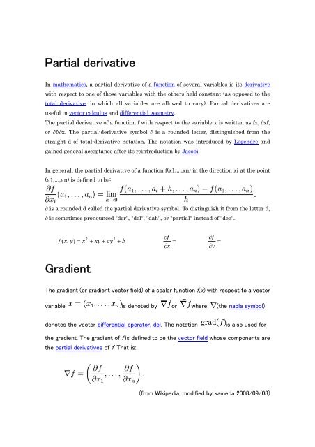
Partial <strong>derivative</strong><br />
In mathematics, a partial <strong>derivative</strong> of a function of several variables is its <strong>derivative</strong><br />
with respect to one of those variables with the others held constant (as opposed to the<br />
<strong>total</strong> <strong>derivative</strong>, in which all variables are allowed to vary). Partial <strong>derivative</strong>s are<br />
useful in vector calculus and differential geometry.<br />
The partial <strong>derivative</strong> of a function f with respect to the variable x is written as fx, ∂xf,<br />
or ∂f/∂x. The partial-<strong>derivative</strong> symbol ∂ is a rounded letter, distinguished from the<br />
straight d of <strong>total</strong>-<strong>derivative</strong> notation. The notation was introduced by Legendre and<br />
gained general acceptance after its reintroduction by Jacobi.<br />
In general, the partial <strong>derivative</strong> of a function f(x1,...,xn) in the direction xi at the point<br />
(a1,...,an) is defined to be:<br />
∂ is a rounded d called the partial <strong>derivative</strong> symbol. To distinguish it from the letter d,<br />
∂ is sometimes pronounced "der", "del", "dah", or "partial" instead of "dee".<br />
2<br />
2<br />
∂f<br />
f ( x,<br />
y)<br />
= x + xy + ay + b<br />
=<br />
∂x<br />
Gradient<br />
∂f<br />
∂y<br />
=<br />
The gradient (or gradient vector field) of a scalar function f(x) with respect to a vector<br />
variable is denoted by or where (the nabla symbol)<br />
denotes the vector differential operator, del. The notation<br />
is also used for<br />
the gradient. The gradient of f is defined to be the vector field whose components are<br />
the partial <strong>derivative</strong>s of f. That is:<br />
(from Wikipedia, modified by kameda 2008/09/08)
Lagrange <strong>multipliers</strong><br />
From Wikipedia, the free encyclopedia (rearranged by kameda, 2008/09/08)<br />
Fig. 1 Fig. 2<br />
Fig. 1. Drawn in red is the locus (contour) of points satisfying the constraint g(x,y) = c. Drawn in<br />
blue are contours of f. Arrows represent the gradient, which points in a direction normal to the<br />
contour.<br />
Fig. 2. Same problem as above as three-dimensional visualization, assuming that we want to<br />
maximize f(x,y).<br />
In mathematical optimization problems, the method of Lagrange <strong>multipliers</strong>, named after Joseph<br />
Louis Lagrange, is a method for finding the extrema of a function of several variables subject to<br />
one or more constraints; it is the basic tool in nonlinear constrained optimization.<br />
Simply put, the technique is able to determine where on a particular set of points (such as a circle,<br />
sphere, or plane) a particular function is the smallest (or largest).<br />
More formally, Lagrange <strong>multipliers</strong> compute the stationary points of the constrained function. By<br />
Fermat's theorem, extrema occur either at these points, or on the boundary, or at points where<br />
the function is not differentiable.<br />
It reduces finding stationary points of a constrained function in n variables with k constraints to<br />
finding stationary points of an unconstrained function in n+k variables. The method introduces a<br />
new unknown scalar variable (called the Lagrange multiplier) for each constraint, and defines a<br />
new function (called the Lagrangian) in terms of the original function, the constraints, and the<br />
Lagrange <strong>multipliers</strong>.<br />
Introduction<br />
Consider a two-dimensional case. Suppose we have a function f(x,y) we wish to maximize or<br />
minimize subject to the constraint
where c is a constant. We can visualize contours of f given by<br />
for various values of d n , and the contour of g given by g(x,y) = c.<br />
Suppose we walk along the contour line with g = c. In general the contour lines of f and g may be<br />
distinct, so traversing the contour line for g = c could intersect with or cross the contour lines of<br />
f. This is equivalent to saying that while moving along the contour line for g = c the value of f can<br />
vary. Only when the contour line for g = c touches contour lines of f tangentially, we do not<br />
increase or decrease the value of f - that is, when the contour lines touch but do not cross.<br />
This occurs exactly when the tangential component of the <strong>total</strong> <strong>derivative</strong> vanishes: ,<br />
which is at the constrained stationary points of f (which include the constrained local extrema,<br />
assuming f is differentiable). Computationally, this is when the gradient of f is normal to the<br />
constraint(s): when for some scalar λ (where is the gradient). Note that the<br />
constant λ is required because, even though the directions of both gradient vectors are equal,<br />
the magnitudes of the gradient vectors are most likely not equal.<br />
A familiar example can be obtained from weather maps, with their contour lines for temperature<br />
and pressure: the constrained extrema will occur where the superposed maps show touching lines<br />
(isopleths).<br />
Geometrically we translate the tangency condition to saying that the gradients of f and g are<br />
parallel vectors at the maximum, since the gradients are always normal to the contour lines. Thus<br />
we want points (x,y) where g(x,y) = c and<br />
where<br />
,<br />
To incorporate these conditions into one equation, we introduce an auxiliary function<br />
and solve
.<br />
Justification<br />
As discussed above, we are looking for stationary points of f seen while travelling on the level set<br />
g(x,y) = c. This occurs just when the gradient of f has no component tangential to the level sets of<br />
g. This condition is equivalent to for some λ. Stationary<br />
points (x,y,λ) of F also satisfy g(x,y) = c as can be seen by considering the <strong>derivative</strong> with<br />
respect to λ.<br />
Caveat: extrema versus stationary points<br />
Be aware that the solutions are the stationary points of the Lagrangian F, and are saddle points:<br />
they are not necessarily extrema of F. F is unbounded: given a point (x,y) that doesn't lie on the<br />
constraint, letting<br />
makes F arbitrarily large or small. However, under certain stronger<br />
assumptions, as we shall see below, the strong Lagrangian principle holds, which states that the<br />
maxima of f maximize the Lagrangian globally.<br />
A more general formulation: The weak Lagrangian principle<br />
Denote the objective function by and let the constraints be given by , perhaps<br />
by moving constants to the left, as in<br />
. The domain of f should be an open<br />
set containing all points satisfying the constraints. Furthermore, f and the g k must have<br />
continuous first partial <strong>derivative</strong>s and the gradients of the g k must not be zero on the domain. [1]<br />
Now, define the Lagrangian, Λ, as<br />
k is an index for variables and functions associated with a particular constraint, k.<br />
without a subscript indicates the vector with elements , which are taken to be<br />
independent variables.<br />
Observe that both the optimization criteria and constraints g k (x) are compactly encoded as<br />
stationary points of the Lagrangian:<br />
and<br />
if and only if<br />
means to take the gradient only with respect to each element in the vector ,<br />
instead of all variables.
implies g k = 0.<br />
Collectively, the stationary points of the Lagrangian,<br />
,<br />
give a number of unique equations <strong>total</strong>ing the length of plus the length of .<br />
Interpretation of λ i<br />
Often the Lagrange <strong>multipliers</strong> have an interpretation as some salient quantity of interest. To see<br />
why this might be the case, observe that:<br />
So, λ k is the rate of change of the quantity being optimized as a function of the constraint<br />
variable. As examples, in Lagrangian mechanics the equations of motion are derived by finding<br />
stationary points of the action, the time integral of the difference between kinetic and potential<br />
energy. Thus, the force on a particle due to a scalar potential,<br />
, can be interpreted<br />
as a Lagrange multiplier determining the change in action (transfer of potential to kinetic energy)<br />
following a variation in the particle's constrained trajectory. In economics, the optimal profit to a<br />
player is calculated subject to a constrained space of actions, where a Lagrange multiplier is the<br />
value of relaxing a given constraint (e.g. through bribery or other means).<br />
Examples<br />
Very simple example<br />
Suppose you wish to maximize f(x,y) = x + y subject to the constraint x 2 + y 2 = 1. The constraint is<br />
the unit circle, and the level sets of f are diagonal lines (with slope -1). Then, where is the<br />
maximum and how much is it
Fig. 3. Illustration of the constrained optimization problem.<br />
Simple example<br />
Suppose you want to find the maximum values for<br />
with the condition that the x and y coordinates lie on the circle around the origin with radius √3,<br />
that is,<br />
Again, where is the maximum and how much is it<br />
Fig. 4. Illustration of the constrained optimization problem.
Suppose you want to find the maximum values for<br />
with the condition that the x and y coordinates lie on the circle around the origin with radius √3,<br />
that is,<br />
Again, where is the maximum and how much is it<br />
Example: entropy<br />
Suppose we wish to find the discrete probability distribution with maximal information entropy.<br />
Then<br />
Of course, the sum of these probabilities equals 1, so our constraint is g(p) = 1 with<br />
We can use Lagrange <strong>multipliers</strong> to find the point of maximum entropy (depending on the<br />
probabilities).<br />
• This page was last modified on 7 September 2008, at 04:03.<br />
• All text is avai<strong>lab</strong>le under the terms of the GNU Free Documentation License. (See<br />
Copyrights for details.)<br />
Wikipedia® is a registered trademark of the Wikimedia Foundation, Inc., a U.S. registered<br />
501(c)(3) tax-deductible nonprofit charity.
Support vector machine<br />
From Wikipedia, the free encyclopedia (rearranged by kameda, 2008/09/08)<br />
Support vector machines (SVMs) are a set of related supervised learning methods used<br />
for classification and regression. Viewing input data as two sets of vectors in an<br />
n-dimensional space, an SVM will construct a separating hyperplane in that space, one<br />
which maximizes the margin between the two data sets. To calculate the margin, two<br />
parallel hyperplanes are constructed, one on each side of the separating hyperplane,<br />
which are "pushed up against" the two data sets. Intuitively, a good separation is<br />
achieved by the hyperplane that has the largest distance to the neighboring datapoints<br />
of both classes, since in general the larger the margin the better the generalization error<br />
of the classifier.<br />
Motivation<br />
H3 doesn't separate the 2 classes. H1 does, with<br />
a small margin and H2 with the maximum<br />
margin.<br />
Classifying data is a common need in machine<br />
learning. Suppose some given data points each<br />
belong to one of two classes, and the goal is to<br />
decide which class a new data point will be in. In<br />
the case of support vector machines, a data<br />
point is viewed as a p-dimensional vector (a list of p numbers), and we want to know<br />
whether we can separate such points with a p − 1-dimensional hyperplane. This is<br />
called a linear classifier. There are many hyperplanes that might classify the data.<br />
However, we are additionally interested in finding out if we can achieve maximum<br />
separation (margin) between the two classes. By this we mean that we pick the<br />
hyperplane so that the distance from the hyperplane to the nearest data point is<br />
maximized. That is to say that the nearest distance between a point in one separated<br />
hyperplane and a point in the other separated hyperplane is maximized. Now, if such a<br />
hyperplane exists, it is clearly of interest and is known as the maximum-margin<br />
hyperplane and such a linear classifier is known as a maximum margin classifier.
Formalization<br />
We are given some training data, a set of points of the form<br />
where the c i is either 1 or −1, indicating the class to which the point belongs. Each<br />
is a p-dimensional real vector. We want to give the maximum-margin hyperplane<br />
which divides the points having c i = 1 from those having c i = − 1. Any hyperplane can<br />
be written as the set of points satisfying<br />
Maximum-margin hyperplane and margins for a<br />
SVM trained with samples from two classes.<br />
Samples on the margin are called the support<br />
vectors.<br />
The vector is a normal vector: it is<br />
perpendicular to the hyperplane. The parameter<br />
determines the offset of the hyperplane from<br />
the origin along the normal vector .<br />
We want to choose the and b to maximize the margin, or distance between the<br />
parallel hyperplanes that are as far apart as possible while still separating the data.<br />
These hyperplanes can be described by the equations<br />
and<br />
Note that if the training data are linearly separable, we can select the two hyperplanes<br />
of the margin in a way that there are no points between them and then try to maximize<br />
their distance. By using geometry, we find the distance between these two<br />
hyperplanes is , so we want to minimize . As we also have to prevent data<br />
points falling into the margin, we add the following constraint: for each i either<br />
for<br />
for the first class or
for<br />
of the second.<br />
This can be rewritten as:<br />
We can put this together to get the optimization problem:<br />
choose<br />
to minimize<br />
subject to<br />
Primal Form<br />
The optimization problem presented in the preceding section is hard because it<br />
depends on the absolute value of |w|. The reason being that it is a non-convex<br />
optimization problem, which are known to be much more difficult to solve than convex<br />
optimization problems. Fortunately it is possible to alter the equation by substituting<br />
||w|| with<br />
without changing the solution (the minimum of the original and the<br />
modified equation have the same w and b). This is a quadratic programming (QP)<br />
optimization problem. More clearly,<br />
minimize , subject to .<br />
The factor of 1/2 is used for mathematical convenience. This problem can now be<br />
solved by standard quadratic programming techniques and programs.<br />
Dual Form<br />
Writing the classification rule in its unconstrained dual form reveals that the maximum<br />
margin hyperplane and therefore the classification task is only a function of the<br />
support vectors, the training data that lie on the margin. The dual of the SVM can be<br />
shown to be:
subject to<br />
, and<br />
where the α terms constitute a dual representation for the weight vector in terms of<br />
the training set:<br />
Extensions to the linear SVM<br />
Soft margin<br />
In 1995, Corinna Cortes and Vladimir Vapnik suggested a modified maximum margin<br />
idea that allows for mis<strong>lab</strong>eled examples. [2] If there exists no hyperplane that can split<br />
the "yes" and "no" examples, the Soft Margin method will choose a hyperplane that<br />
splits the examples as cleanly as possible, while still maximizing the distance to the<br />
nearest cleanly split examples. This work popularized the expression Support Vector<br />
Machine or SVM. The method introduces slack variables, ξ, i which measure the<br />
degree of misclassification of the datum x i<br />
.<br />
The objective function is then increased by a function which penalises non-zero ξ,<br />
i<br />
and the optimisation becomes a trade off between a large margin, and a small error<br />
penalty. If the penalty function is linear, the equation (3) now transforms to<br />
This constraint in (2) along with the objective of minimizing |w| can be solved using<br />
Lagrange <strong>multipliers</strong>. The key advantage of a linear penalty function is that the slack
variables vanish from the dual problem, with the constant C appearing only as an<br />
additional constraint on the Lagrange <strong>multipliers</strong>. Non-linear penalty functions have<br />
been used, particularly to reduce the effect of outliers on the classifier, but unless<br />
care is taken, the problem becomes non-convex, and thus it is considerably more<br />
difficult to find a global solution.<br />
Non-linear classification<br />
The original optimal hyperplane algorithm proposed by Vladimir Vapnik in 1963 was a<br />
linear classifier. However, in 1992, Bernhard Boser, Isabelle Guyon and Vapnik<br />
suggested a way to create non-linear classifiers by applying the kernel trick (originally<br />
proposed by Aizerman et al.. [3] ) to maximum-margin hyperplanes. [4] The resulting<br />
algorithm is formally similar, except that every dot product is replaced by a non-linear<br />
kernel function. This allows the algorithm to fit the maximum-margin hyperplane in the<br />
transformed feature space. The transformation may be non-linear and the<br />
transformed space high dimensional; thus though the classifier is a hyperplane in the<br />
high-dimensional feature space it may be non-linear in the original input space.<br />
If the kernel used is a Gaussian radial basis function, the corresponding feature space<br />
is a Hilbert space of infinite dimension. Maximum margin classifiers are well regularized,<br />
so the infinite dimension does not spoil the results. Some common kernels include,<br />
• Polynomial (homogeneous):<br />
• Polynomial (inhomogeneous):<br />
• Radial Basis Function: , for γ > 0<br />
• Gaussian Radial basis function:<br />
• Sigmoid: , for some (not every) κ > 0 and c <<br />
0<br />
This page was last modified on 27 August 2008, at 17:49. All text is avai<strong>lab</strong>le under the<br />
terms of the GNU Free Documentation License. (See Copyrights for details.)