Uzawa method on semi-staggered grids for unsteady Bingham ...
Uzawa method on semi-staggered grids for unsteady Bingham ...
Uzawa method on semi-staggered grids for unsteady Bingham ...

You also want an ePaper? Increase the reach of your titles
YUMPU automatically turns print PDFs into web optimized ePapers that Google loves.
Russ. J. Numer. Anal. Math. Modelling, Vol. 24, No. 6, pp. 543–563 (2009)<br />
DOI 10.1515/ RJNAMM.2009.034<br />
cde Gruyter 2009<br />
<str<strong>on</strong>g>Uzawa</str<strong>on</strong>g> <str<strong>on</strong>g>method</str<strong>on</strong>g> <strong>on</strong> <strong>semi</strong>-<strong>staggered</strong> <strong>grids</strong> <strong>for</strong> <strong>unsteady</strong><br />
<strong>Bingham</strong> media flows<br />
L. V. MURAVLEVA£and E. A. MURAVLEVA †<br />
Abstract — A finite difference scheme <strong>on</strong> <strong>semi</strong>-<strong>staggered</strong> <strong>grids</strong> is used <strong>for</strong> numerical simulati<strong>on</strong> of<br />
<strong>unsteady</strong> flows of an incompressible viscoplastic <strong>Bingham</strong> medium. The Duvaut–Li<strong>on</strong>s variati<strong>on</strong>al<br />
inequality is c<strong>on</strong>sidered as a mathematical model. The c<strong>on</strong>vergence of the <str<strong>on</strong>g>Uzawa</str<strong>on</strong>g> <str<strong>on</strong>g>method</str<strong>on</strong>g> is proved.<br />
The efficiency of the <str<strong>on</strong>g>method</str<strong>on</strong>g> is dem<strong>on</strong>strated <strong>on</strong> a model problem with a known exact soluti<strong>on</strong> (plane<br />
Poiseuille flow) and <strong>on</strong> the <strong>unsteady</strong> driven cavity problem.<br />
1. Statement of the problem<br />
There exists a number of materials behaving as a viscoplastic medium (<strong>Bingham</strong><br />
medium), namely, i.e., the medium behaves as a rigid body below some limit stress<br />
value and above this level it behaves as an incompressible viscous fluid. A variati<strong>on</strong>al<br />
statement <strong>for</strong> the flows of viscoplastic media was first proposed by Il’yushin<br />
[11]. In [16] the existence and uniqueness theorems were proved <strong>for</strong> the problem<br />
of the flow in a pipe and a qualitative study of flow specifics was per<strong>for</strong>med.<br />
M<strong>on</strong>ograph [8] c<strong>on</strong>tains strict mathematical analysis of variati<strong>on</strong>al inequalities corresp<strong>on</strong>ding<br />
to this model.<br />
Let Ω be a bounded domain in R dd23and Γ be a locally Lipschitz boundary<br />
of the domain Ω. A flow of an incompressible viscoplastic medium during the<br />
σ Ω¢´0Tµ<br />
time interval´0Tµis described by the following system of equati<strong>on</strong>s and c<strong>on</strong>stitutive<br />
relati<strong>on</strong>s:<br />
ρ∂v<br />
∂t·´v¡∇µv∇¡σ·f∇¡v0 s D´vµ Γ¢´0Tµ<br />
in (1.1)<br />
pI·ττ2µD´vµ·σ s<br />
D´vµD´vµ0<br />
(1.2)<br />
τσ D´vµ0<br />
v´0µv 0 in Ω∇¡v 00v0 <strong>on</strong> (1.3)<br />
£Moscow State University, Faculty of Mechanics and Mathematics, Moscow 119991, Russia<br />
† Institute of Numerical Mathematics, Russian Academy of Sciences, Moscow 119333, Russia<br />
The work was partially supported by the Russian Foundati<strong>on</strong> <strong>for</strong> Basic Research (08–01–00353,<br />
09–01–00565).
544 L. V. Muravleva and E. A. Muravleva<br />
Equati<strong>on</strong>s (1.1)–(1.3) use the standard notati<strong>on</strong>s: ρµσ s are positive c<strong>on</strong>stants,<br />
namely the density, the viscosity coefficient, and the yield stress of the <strong>Bingham</strong><br />
medium, respectively (sometimes we use τ s as shear yield stress, σ sτ sÔ2); v is the<br />
unknown velocity field, f is the given field of external <strong>for</strong>ces; σ is the stress tensor,<br />
τ is the deviator of the stress tensor, and p is the pressure, D´vµ∇v·´∇vµT℄2<br />
is the strain rate tensor with the normD´vµ<br />
0¨xt¾Ω¢´0Tµ<br />
∑ d i1 ∑ d j1 D i j´vµD j´vµ¡12 i .<br />
System (1.1)–(1.3) holds in the domain of moti<strong>on</strong> (i.e.,D´vµ0) and, generally<br />
speaking, has no meaning in the rigid z<strong>on</strong>e Ω<br />
typical peculiarity in problems of viscoplastic media flows<br />
D´vµ´xtµ0©. The<br />
is the necessity to c<strong>on</strong>struct soluti<strong>on</strong>s in domains with unknown boundaries. This<br />
causes significant difficulties in c<strong>on</strong>structi<strong>on</strong> of efficient <str<strong>on</strong>g>method</str<strong>on</strong>g>s <strong>for</strong> their study.<br />
The main difficulty in numerical simulati<strong>on</strong> of the flow of a viscoplastic medium is<br />
related to n<strong>on</strong>differentiability of c<strong>on</strong>stitutive relati<strong>on</strong>s. One of the most successful<br />
techniques to overcome the menti<strong>on</strong>ed difficulties is using the theory of variati<strong>on</strong>al<br />
inequalities [8, 10, 12]. The finite element <str<strong>on</strong>g>method</str<strong>on</strong>g> is traditi<strong>on</strong>ally employed as the<br />
discretizati<strong>on</strong> technique [7] in numerical simulati<strong>on</strong> of <strong>Bingham</strong> media. In this paper<br />
we apply the finite-difference scheme from [19–23] <strong>for</strong> determinati<strong>on</strong> of an<br />
approximate soluti<strong>on</strong>. We c<strong>on</strong>sider the numerical soluti<strong>on</strong> of the <strong>unsteady</strong> driven<br />
cavity problem <strong>for</strong> a <strong>Bingham</strong> medium as a model example. The obtained results<br />
are compared to those known from the literature.<br />
2. Variati<strong>on</strong>al inequality<br />
Duvaut and Li<strong>on</strong>s [8] proposed the problem <strong>on</strong> the solvability of following variati<strong>on</strong>al<br />
inequality (2.1) (with c<strong>on</strong>diti<strong>on</strong>s (2.2),(2.3)) as a strict <strong>for</strong>mulati<strong>on</strong> of problem<br />
(1.1)–(1.3) of a viscoplastic flow: determine v´tµ¾´H0´Ωµµd 1 so that <strong>for</strong> each<br />
t¾´0Tµthe following inequality holds:<br />
∂v<br />
ρΩ ∂t¡´u v´tµµdx·ρΩ´v´tµ¡∇µv´tµ¡´u v´tµµdx<br />
D´v´tµµµdx<br />
(2.1)<br />
sΩ´D´uµ 1´Ωµµd∇¡u0 ·2µΩ<br />
D´v´tµµ:D´u v´tµµdx·σ Ω f´tµ¡´u v´tµµdxu¾U ∇¡v´tµ0 in Ωv´0µv 0 in Ωv´tµ0 Uu¾´H (2.3)<br />
i<br />
<strong>on</strong><br />
i<br />
Γ (2.2)<br />
where A : B∑ d i1 ∑ d j1 a i jb i j <strong>for</strong> all tensors A´a jµand B´b jµof the sec<strong>on</strong>d<br />
order. Inequality (2.1) ‘automatically’ includes the problem <strong>on</strong> a ‘free boundary’.<br />
In our case it is the surface separating the domain in which the flow is described<br />
by equati<strong>on</strong> (1.1) from the domain where the medium moves as a rigid body. The<br />
following theorem <strong>on</strong> multipliers was also proved in [8].
∂t·´v¡∇µv<br />
<str<strong>on</strong>g>Uzawa</str<strong>on</strong>g> <str<strong>on</strong>g>method</str<strong>on</strong>g> <strong>on</strong> <strong>semi</strong>-<strong>staggered</strong> <strong>grids</strong> 545<br />
Theorem 2.1 [8]. Let v be a soluti<strong>on</strong> to problem (2.1)–(2.3). Then there exists<br />
a tensor-valued functi<strong>on</strong> λλ i j1ijd Ω¢´0Tµ Ω¢´0Tµ<br />
such that<br />
Γ¢´0Tµ<br />
λ¾´L ∞´Ωµµd¢dλλ Tλ1<br />
λ : D´vµD´vµa.e. in (2.4)<br />
ρ∂v<br />
µv σ s ∇¡λ·∇pf in (2.5)<br />
∇¡v0 in Ω¢´0Tµv´0µv 0 in Ωv0 <strong>on</strong> (2.6)<br />
If, <strong>on</strong> the c<strong>on</strong>trary, the triplevpλsatisfies relati<strong>on</strong>s (2.4)–(2.6), then v is the<br />
soluti<strong>on</strong> to problem (2.1)–(2.3).<br />
3. Discretizati<strong>on</strong> of problem (2.1)–(2.3) in time<br />
Suppose the flow is slow, i.e., we can neglect the c<strong>on</strong>vective term (the Stokes approximati<strong>on</strong>).<br />
Following [7], we use the well-known backward Euler scheme <strong>for</strong><br />
time discretizati<strong>on</strong> of problem (2.1)–(2.3). Lett0 be a c<strong>on</strong>stant time step. Assume<br />
v 0v 0<br />
kµdxu¾U<br />
then <strong>for</strong> k1 we compute v k from v k 1 as the soluti<strong>on</strong> to the following inequality<br />
(here and further f kf´ktµ)<br />
ρtΩ´v k v k 1µ¡´u v kµdx·2µΩ D´v kµ:D´u v k¡´u<br />
f v<br />
We introduce αρtff k 1 , in what follows<br />
sΩ´D´uµ<br />
we omit the subscript k.<br />
Then in the new notati<strong>on</strong>s we have<br />
αΩ<br />
v¡´u D´vµ:D´u vµdx·σ vµdx·2µΩ<br />
D´vµµdx<br />
(3.1)<br />
sΩ´D´uµ ·σ k·αv<br />
Ω f¡´u vµdxu¾U<br />
D´v kµµdxΩ<br />
4. <str<strong>on</strong>g>Uzawa</str<strong>on</strong>g>’s algorithm<br />
Numerical <str<strong>on</strong>g>method</str<strong>on</strong>g>s <strong>for</strong> solving variati<strong>on</strong>al inequality (3.1) are based <strong>on</strong> the following<br />
approach. Introduce the functi<strong>on</strong>al<br />
dx·σ sΩD´uµdx f¡udx (4.1)<br />
Ω<br />
J´uµα<br />
2Ωu2 dx·µΩD´uµ2
J´uµ<br />
546 L. V. Muravleva and E. A. Muravleva<br />
The functi<strong>on</strong>al J´uµis strictly c<strong>on</strong>vex, but is not differentiable because of the term<br />
σ sÊΩD´uµdx. The soluti<strong>on</strong> v of problem (3.1) is the minimiser of the functi<strong>on</strong>al J<br />
<strong>on</strong> U [10]:<br />
vargmin<br />
(4.2)<br />
u¾U Taking into account inequality (2.4), <strong>for</strong> the integral of the c<strong>on</strong>tracti<strong>on</strong> λ : D´uµ,<br />
0´Ωµµd 1<br />
λ : D´vµdxΩD´vµdx<br />
Ω<br />
λ :<br />
Ω<br />
D´uµdxΩλD´uµdxΩD´uµdxu¾´H<br />
we get the following relati<strong>on</strong>:<br />
ΩD´vµdxsup λ : D´vµdx (4.3)<br />
λ¾ΛΩ<br />
where Λλλ¾´L∞´Ωµµd¢dλλ Tλ1a.e. <strong>on</strong> Ω. Further, substituting<br />
expressi<strong>on</strong> (4.3) into the functi<strong>on</strong>al, we have<br />
s sup<br />
f¡udx<br />
dx·σ λ : D´uµdx<br />
λ¾ΛΩ<br />
Ω<br />
or<br />
dx·σ λ : D´uµdx sΩ<br />
f¡udx<br />
Ω<br />
Introduce the Lagrange functi<strong>on</strong>alÄ:´H 1´Ωµµd¢´L 2´Ωµµd¢dÊcorresp<strong>on</strong>ding<br />
to (4.1) as<br />
dx·σ η : D´uµdx f¡udx(4.4)<br />
sΩ<br />
Ω<br />
inf<br />
u¾Uα<br />
2Ωu2 dx·µΩD´uµ2<br />
inf sup<br />
u¾U λ¾Λα<br />
2Ωu2 dx·µΩD´uµ2<br />
Ä´u;ηµα<br />
2Ωu2 dx·µΩD´uµ2<br />
In accordance with the minimax theorem [9, 10], the pair´vλµis a saddle point of<br />
the Lagrange functi<strong>on</strong>alÄ´u;ηµ<strong>on</strong> U¢Λ:<br />
´vλµ¾U B¢ΛÄ´v;ηµÄ´v;λµÄ´u;λµ´uηµ¾U¢Λ (4.5)<br />
and the first comp<strong>on</strong>ent of the pair v is uniquely determined and it is the soluti<strong>on</strong> to<br />
optimizati<strong>on</strong> problem (4.2). The first inequality of (4.5) is equivalent [9, 26] to the<br />
equati<strong>on</strong><br />
Ω¢´0Tµ λ´tµP Λ´λ´tµ·rσ s D´v´tµµµr0a.e. <strong>on</strong><br />
(4.6)
Λ´qµ´xµ´q´xµ<br />
<str<strong>on</strong>g>Uzawa</str<strong>on</strong>g> <str<strong>on</strong>g>method</str<strong>on</strong>g> <strong>on</strong> <strong>semi</strong>-<strong>staggered</strong> <strong>grids</strong> 547<br />
where P Λ :´L∞´Ωµµd¢dΛ is the operator of orthog<strong>on</strong>al projecti<strong>on</strong> defined by the<br />
following expressi<strong>on</strong>:<br />
2µ∇¡D´vµ<br />
q´xµ1<br />
D´vµµ<br />
P <strong>on</strong><br />
q´xµq´xµq´xµ1a.e. Ωq¾´L This remark plays an important role in computati<strong>on</strong>s. Due to Theorem 2.1, the pair<br />
´vλµsatisfies the following relati<strong>on</strong>s:<br />
αv σ s ∇¡λ·∇pf∇¡v0 in Ωv0 <strong>on</strong> Γ (4.8)<br />
λP Λ´λ·rσ s (4.9)<br />
Based <strong>on</strong> (4.8)–(4.9), nµ we c<strong>on</strong>struct the following algorithm, which is the <str<strong>on</strong>g>Uzawa</str<strong>on</strong>g><br />
algorithm applied to the saddle-point problem withÄ´u;ηµ:<br />
λ 0¾Λ is given (arbitrarily) (4.10)<br />
<strong>for</strong> n0, assuming that λ n´¾Λµis nµµ known, we compute v n as an element of U that<br />
is the saddle point of the LagrangianÄ´u;ηµ, i.e., as the soluti<strong>on</strong> to the problem<br />
αv n 2µ∇¡D´v σ s ∇¡λ n·∇p nf∇¡v0 in Ωv0 <strong>on</strong> Γ (4.11)<br />
after that, the new approximati<strong>on</strong> λ n·1 is determined as<br />
λ n·1P Λ´λ n·rσ s D´v (4.12)<br />
The following remark presents several useful <strong>for</strong>mulae we need further in the<br />
proof of the theorem.<br />
∞´Ωµµd¢d (4.7)<br />
Remark 4.1. C<strong>on</strong>sidering the velocity gradient ∇v as a sec<strong>on</strong>d-order tensor, represent<br />
it in the <strong>for</strong>m of a sum of the symmetric strain rate tensor D´vµand the antisymmetric<br />
rotati<strong>on</strong> velocity tensor w´vµ1<br />
2¢∇v ´∇vµT£with the comp<strong>on</strong>ents<br />
´w i j1<br />
2´∇ i v j ∇ j v iµµ. Then, taking into account that the c<strong>on</strong>tracti<strong>on</strong> of the symmetric<br />
and antisymmetric tensors is equal to zero, we get the following relati<strong>on</strong>s:<br />
D´vµ:w´vµ0λ : w´vµ0´λλ j´vµµ<br />
In additi<strong>on</strong>, <strong>for</strong> D´vµ:∇v and λ : ∇v we have<br />
i<br />
d<br />
∑ D i j´vµD j´vµD´vµ2<br />
D´vµ<br />
i<br />
ij1<br />
:<br />
D´vµ:∇vd ∑ D i j´vµ∇ i v jd ∑ D i j´vµ´D ij1<br />
ij1<br />
λ : ∇vd ∑ λ i j´D i j´vµ·w ij1<br />
j´vµµd i<br />
Tµ<br />
i j´vµ·w<br />
∑ λ i j D i j´vµλ ij1
548 L. V. Muravleva and E. A. Muravleva<br />
Prove the theorem of c<strong>on</strong>vergence of <str<strong>on</strong>g>Uzawa</str<strong>on</strong>g>’s <str<strong>on</strong>g>method</str<strong>on</strong>g> <strong>for</strong> problem (2.1)–(2.3).<br />
Theorem 4.1. Suppose the c<strong>on</strong>diti<strong>on</strong><br />
0r4µσ s 2 (4.13)<br />
holds. Then <strong>for</strong> the sequencevnn0 generated by algorithm (4.10)–(4.12) we have<br />
lim vnv in´H 0´Ωµµd 1<br />
n·∞ where v is the soluti<strong>on</strong> nµ n<br />
to (4.8)–(4.9).<br />
Proof. Letvλbe the soluti<strong>on</strong> to (4.8)–(4.9). Assuming v nvn vp p n p and λ nλ n λ and taking into account that the projecti<strong>on</strong> operator P Λ<br />
satisfies the relati<strong>on</strong>P Λ x P Λ 2´Ωµµd¢d yx y, as a result of subtracti<strong>on</strong> of (4.8)–(4.9)<br />
from (4.11)–(4.12), we get that <strong>for</strong> all n0 we have<br />
αv n 2µ∇¡D´v σ s ∇¡λ n·∇pn0∇¡vn0 in Ωvn0 <strong>on</strong> Γ (4.14)<br />
n·1´L λ 2´Ωµµd¢dλ n·rσ s D´vnµ´L (4.15)<br />
Inequality (4.15) implies<br />
λ n·12´L2´Ωµµd¢dλ n2´L2´Ωµµd¢d·2rσ nD´v s´λ nµµ·r 2 σsD´v 2 nµ2´L 2´Ωµµd¢d<br />
which gives<br />
nµ nµµ<br />
nµ<br />
λ n2´L r 2 σsD´v 2 nµ2´L 2rσ s´λ nD´v 2´Ωµµd¢d 2´Ωµµd¢d (4.16)<br />
Multiply (4.14) by v n :<br />
´αv nv 2µ´∇¡D´v nµv σ nv s´∇¡λ nµ·´∇p nv nµ0<br />
integrate by parts, nµ and take into nµ nµ account Remark<br />
nµµ nµµ<br />
4.1:<br />
αv n2´L 2´Ωµµ2·2µ´D´v nµD´v nµµ·σ s´λ nD´v nµµ0<br />
because of<br />
´∇¡D´v nµv ´D´v nµ∇v ´D´v nµD´v D´v nµ2´L 2´Ωµµd¢d<br />
´∇¡λ nv ´λ n∇v nD´v ´λ<br />
For all v such that v¾´H 0´Ωµµd∇¡v0 1 we have 2D´vµ2´L because of ∇v2´L2´Ωµµd¢d 2´Ωµµd¢d λ n·12´L<br />
2´Ωµµd¢d
<str<strong>on</strong>g>Uzawa</str<strong>on</strong>g> <str<strong>on</strong>g>method</str<strong>on</strong>g> <strong>on</strong> <strong>semi</strong>-<strong>staggered</strong> <strong>grids</strong><br />
jµ<br />
549<br />
d<br />
2´D´vµD´vµµ2´D´vµ∇vµ2 ∑<br />
jµd i j∇ i v ∑<br />
jµ<br />
i v j·∇ j v i∇ i v<br />
ij1´D ij1´∇ d<br />
∑ i ∇ j v iv ij1´∇ 2´Ωµµd¢d 2´Ωµµd¢d<br />
j∇v2´L Thus,<br />
nµµ 2rαv n2´L 2´Ωµµd·4rµD´v nµ2´L 2rσ nD´v s´λ (4.17)<br />
Taking into account relati<strong>on</strong>s (4.16) and (4.17), we get<br />
λ n2´L n·12´L λ 2´Ωµµd¢d 2´Ωµµd¢d<br />
r 2 σsD´v 2 nµ2´L 2´Ωµµd¢d·2rαv n2´L 2´Ωµµd·4rµD´v nµ2´L 2´Ωµµd¢d 2r´D´v nµ2´L 2´Ωµµd¢d´2µ rσs2µ·αv 2 n2´L 2´Ωµµdµ 2´Ωµµdµ<br />
2´Ωµµd r´∇´v nµ2´L 2´Ωµµd¢d´2µ rσs2µ·2αv 2 n2´L α<br />
rσ<br />
r∇´v nµ2´L s<br />
2 rσ 2<br />
µ2<br />
2µ·α2<br />
s s<br />
2µ·rσ 2<br />
2µv<br />
n2´L 2´Ωµµd¢d rσs<br />
2 r2<br />
2µ´µ∇´v nµ2´L 2´Ωµµd¢d·αv n2´L (4.18)<br />
C<strong>on</strong>diti<strong>on</strong> (4.13) implies r´2 rσs2µµ0 2 (where, as we have seen,<br />
ρ∆t). Relati<strong>on</strong>s (4.18) imply that the sequence λ n2´L2´Ωµµd¢d¡n0 decreases and<br />
hence c<strong>on</strong>verges to some limit. The latter means<br />
lim<br />
(4.19)<br />
n·∞ Combining (4.18) and (4.19), we get lim n·∞ v n0 in´H1´Ωµµd , namely, the c<strong>on</strong>vergence<br />
ofvnn0 to v in´H0´Ωµµd 1 .<br />
Remark 4.2. Estimate (4.13) determines the interval of admissible values of the<br />
parameter r providing the c<strong>on</strong>vergence of <str<strong>on</strong>g>Uzawa</str<strong>on</strong>g>’s algorithm (projecti<strong>on</strong> <str<strong>on</strong>g>method</str<strong>on</strong>g>)<br />
to the soluti<strong>on</strong>. But in the proof of Theorem 4.1 we neglect the term αv n2´L 2´Ωµµd<br />
d<br />
∑<br />
ij1´∇ i v j∇ i v jµ·d<br />
∑<br />
ij1´∇ j v i∇ i v jµ∇v2<br />
∇v2 d<br />
∑<br />
j1∇ jd<br />
∑<br />
i1∇ i v iv<br />
λ n2´L2´Ωµµd¢d 2´Ωµµd¢d¡0 λ n·12´L<br />
in <strong>for</strong>mula (4.18). Estimate (4.13) allows us to choose a value of r both <strong>for</strong> steady<br />
and <strong>unsteady</strong> problems. For evoluti<strong>on</strong>al problems the range of admissible values of
550 L. V. Muravleva and E. A. Muravleva<br />
the parameter r may be extended a little. According to the Poincaré inequality, the<br />
following relati<strong>on</strong> holds:<br />
γ minv2´L 2´Ωµµd∇v2´L 2´Ωµµd¢d<br />
where γ min<br />
2´Ωµµdµ 2´Ωµµd¡<br />
is the least eigenvalue of the Laplace operator with the homogeneous<br />
Dirichlet boundary c<strong>on</strong>diti<strong>on</strong>s in the domain Ω. Replacing in (4.18) the value<br />
∇´v nµ2´L by a smaller expressi<strong>on</strong> c<strong>on</strong>taining <strong>on</strong>lyvn2´L2´Ωµµd¢d, we get<br />
2´Ωµµd¢d r´∇´v nµ2´L 2´Ωµµd¢d´2µ rσs2µ·2αv 2 n2´L r γ minv n2´L2´Ωµµd¢d´2µ rσs2µ·2αv 2 n2´L rv n2´L2´Ωµµd¢d2µ rσs<br />
2·2α<br />
2<br />
γ minγ<br />
Thus, the extended interval of admissible values <strong>for</strong> the parameter<br />
min<br />
r has the <strong>for</strong>m<br />
0r4σ 2<br />
s´µ·αγ minµ<br />
5. Finite-difference scheme<br />
The <str<strong>on</strong>g>Uzawa</str<strong>on</strong>g> <str<strong>on</strong>g>method</str<strong>on</strong>g> described in Secti<strong>on</strong> 4 is applicable to the finite-difference approximati<strong>on</strong><br />
of variati<strong>on</strong>al inequality (3.1). Further we restrict ourselves to the case<br />
of a rectangular domain Ω. Since the <str<strong>on</strong>g>Uzawa</str<strong>on</strong>g> <str<strong>on</strong>g>method</str<strong>on</strong>g> is justified here in its functi<strong>on</strong>al<br />
<strong>for</strong>m, its applicati<strong>on</strong> to a finite-dimensi<strong>on</strong>al problem cannot be assumed completely<br />
justified. This gap will be filled in <strong>on</strong>e of the <strong>for</strong>thcoming papers. As it was<br />
pointed out in Secti<strong>on</strong> 1, most papers c<strong>on</strong>cerning numerical simulati<strong>on</strong> of a <strong>Bingham</strong><br />
medium use the finite element <str<strong>on</strong>g>method</str<strong>on</strong>g> <strong>for</strong> discretizati<strong>on</strong> [14]. In [19–22] some<br />
difference schemes were proposed, and <strong>on</strong>e of those schemes is used<br />
2in this paper.<br />
Let Ω´01µ2 1<br />
1<br />
and assume h 1N 1<br />
and h 2N 2<br />
<strong>for</strong> given natural N 1N 2<br />
1<br />
. Define<br />
the following grid domains:<br />
¯Ω 1x i j´ih 1jh 2µi0N 1j0N Ω 2x i j´´i·12µh 1´j·12µh 2µi0N 1 1j0N 2<br />
Define the spaces of the grid comp<strong>on</strong>ents of the velocity and pressure functi<strong>on</strong>s<br />
taking real values:<br />
V 0 hv ij´u ijv ijµ´u´x P hp j :p´x i jµx<br />
i<br />
i jµv´x i<br />
i jµµx<br />
j¾Ω 2∑<br />
j0<br />
i<br />
p i<br />
ij<br />
j¾¯Ω 1v 0jv iN 2v N1jv i00<br />
By V h we denote the spaces of the grid vector functi<strong>on</strong>s determined <strong>on</strong>ly at the internal<br />
points of Ω 1 . All comp<strong>on</strong>ents of the strain rate tensor (D h´v hµD h´v hµij)
<str<strong>on</strong>g>Uzawa</str<strong>on</strong>g> <str<strong>on</strong>g>method</str<strong>on</strong>g> <strong>on</strong> <strong>semi</strong>-<strong>staggered</strong> <strong>grids</strong><br />
2<br />
551<br />
and the stress tensor (λ hλ hij) are determined <strong>on</strong> the grid Ω 2 . The corresp<strong>on</strong>ding<br />
space of real grid tensor functi<strong>on</strong>s is denoted by Q h :<br />
Q hq hq hq 11<br />
i j¾Ω For vector grid functi<strong>on</strong>s of the <strong>for</strong>m v h´uvµT determined <strong>on</strong> ¯Ω 1 we define the<br />
scalar product by the <strong>for</strong>mula<br />
1v 1µTv h´u 2µT 2v<br />
hq 12<br />
hq 21<br />
hq 22<br />
h;´q hµijq h´x i jµx<br />
´u hv hµh∑<br />
x i j¾¯Ω 1´u 1 ij u2 ij·v 1 ij v2 ijµh 1 h 2u h´u<br />
<strong>for</strong> scalar functi<strong>on</strong>s determined <strong>on</strong> Ω 2 we use the <strong>for</strong>mula<br />
´p hq hµh∑<br />
x i j¾Ω 2<br />
p ijq ijh 1 h 2<br />
<strong>for</strong> tensor functi<strong>on</strong>s determined <strong>on</strong> Ω 2 we use the <strong>for</strong>mula<br />
´q hλ hµh∑<br />
x i j¾Ω 2´q 11<br />
ijλij·q 11 12<br />
ijλij·q 12 21<br />
ijλij·q 21 22<br />
ijλ 22<br />
2 ijµh 1<br />
h<br />
h<br />
Further in the text we use norms <strong>for</strong> vector, scalar, and tensor grid functi<strong>on</strong>s. All<br />
those norms are calculated based <strong>on</strong> the introduced scalar products:<br />
v hh´v hp hh´p hp hλ hh´λ hλ<br />
hv hµ12<br />
hµ12<br />
hµ12<br />
Define the discrete analogue of the differential divergence operator ∇ h¡:V 0 hP h :<br />
´∇ i·1j·1 u ij·1·u i·1j u ij<br />
h¡v hµiju ·v i·1j·1 v i·1j·v ij·1 v ij<br />
2h 1<br />
2h 2<br />
(5.1)<br />
and the strain rate tensor D h : V 0 hQ h :<br />
i·1j·1 u ij·1·u i·1j u ij<br />
2h 1<br />
hµµijv ´D 22<br />
i·1j·1 v i·1j·v ij·1 v ij<br />
h´v 2h 2<br />
<br />
hµµiju ´D 12<br />
h´v hµµij´D 21<br />
i·1j·1 u i·1j·u ij·1 u ij<br />
h´v 4h 2<br />
·v i·1j·1 v ij·1·v i·1j v ij<br />
4h 1<br />
A direct check verifies that the difference scheme obtained here approximates the<br />
original problem with the orderÇ´h2µ<strong>for</strong> h1<br />
smooth functi<strong>on</strong>s. Define a closed c<strong>on</strong>vex<br />
set Λ h and spaces Q h by<br />
Λ hλ hλ h¾Q hλ hλ T hλ<br />
´D 11<br />
h´v hµµiju
552 L. V. Muravleva and E. A. Muravleva<br />
λ hij´´λ hµ2 11<br />
ij·2´λ hµ2 12<br />
ij·´λ hµ2 22<br />
ijµ12 is the norm of a tensor functi<strong>on</strong> at a point<br />
x i j¾Ω 2<br />
h¡<br />
.<br />
C<strong>on</strong>sider the discrete analogue of the LagrangianÄ´u;ηµ(4.4):<br />
Äh´v hλ hµh 1 h 2α<br />
2<br />
∑´u hµ2·´v hµ2¡·µ<br />
h¡ hµ2¡<br />
∑´D 11<br />
hµ2·´D 22<br />
hµ2·2´D 12<br />
M i j¾Ω 1 M i j¾Ω 2<br />
·σ s ∑ D 11<br />
h λh·D 11 22<br />
h λh·2D 22 12<br />
h λ 12<br />
∑ fh 1 u h·f h 2 v<br />
M i j¾Ω 2 M i j¾Ω 1<br />
In order to find the saddle point of the discrete LagrangianÄh´v hλ hµ, we apply<br />
the discrete versi<strong>on</strong> of algorithm (4.10)–(4.12) in the following <strong>for</strong>m:<br />
λ 0 h¾Λ h is given arbitrarily<br />
given λ n h´¾Λ hµ, n0, we compute v n n·1<br />
h<br />
, after that the new approximati<strong>on</strong> λ h<br />
determined by the following steps.<br />
(5.2)<br />
is<br />
h0<br />
Step 1. Solve´αv n h<br />
µhv n·∇ h p n hσ s ∇ h¡λ n h·f h<br />
∇ h¡vn Step 2. Calculate<br />
(5.3)<br />
then repeat from Step 1.<br />
hµ´ hµ<br />
For the discretizati<strong>on</strong>s´∇ h¡v hµand´D h´v hµµintroduced here and under the<br />
c<strong>on</strong>diti<strong>on</strong> ∇ h¡v h0, the following equality holds:<br />
2´D h´v hµD h´v hµµ´∇ h v h∇ h v hv hv <br />
(5.4)<br />
In this case we obtain the following discrete analogues of the gradient operator<br />
∇ h : P hV h :<br />
hµijp<br />
´∇ ij p i 1j·p ij 1 p i p 1j 1 ij p ij 1·p i 1j p i 1j 1<br />
h p<br />
2h 1 2h 2<br />
(5.5)<br />
and the Laplace operator ∆ h : V 0 hV h<br />
1µ<br />
:<br />
´∆ h v hµij1<br />
4h 2 i·1j·1 2v ij·1·v i 1j·1<br />
1´v ·2v i·1j 4v ij·2v i 1j·v i·1j 1 2v ij 1·v i<br />
1µ<br />
1j ·1<br />
i·1j·1·2v ij·1·v 4h 2 i 1j·1<br />
2´v 2v i·1j 4v ij 2v i 1j·v i·1j 1·2v ij 1·v i 1j<br />
Ifλ n·1<br />
h λ n hε,<br />
λ n·1<br />
hP Λh´λ n h·rσ s D h´v n hµµ
<str<strong>on</strong>g>Uzawa</str<strong>on</strong>g> <str<strong>on</strong>g>method</str<strong>on</strong>g> <strong>on</strong> <strong>semi</strong>-<strong>staggered</strong> <strong>grids</strong> 553<br />
In the case h 1h 2h <strong>for</strong> ∆ h we obtain the so-called ‘shift’ approximati<strong>on</strong>:<br />
´∆ i 1j 1·v i·1j 1·v i·1j·1·v i 1j·1 4v ij<br />
h v hµijv 2h 2 (5.6)<br />
The choice of the parameter r in algorithm (5.2), (5.3) is per<strong>for</strong>med in <strong>for</strong>mal accordance<br />
with Remark 4.2, i.e., we suppose∇ h v n hh c<strong>on</strong>verges to∇ h v hh <strong>for</strong> all r<br />
from the interval<br />
0r4<br />
σsµ·α<br />
2 γ min<br />
Be<strong>for</strong>e proceeding to numerical experiments, let us discuss the algorithm and<br />
the details of its implementati<strong>on</strong>. The sec<strong>on</strong>d step per<strong>for</strong>ms pointwise calculati<strong>on</strong>s<br />
and causes no difficulties. The first step c<strong>on</strong>sists in the soluti<strong>on</strong> of the generalized<br />
Stokes problem with a c<strong>on</strong>stant matrix of the system and a variable right-hand<br />
side. The first iterative <str<strong>on</strong>g>method</str<strong>on</strong>g>s <strong>for</strong> soluti<strong>on</strong> of the stati<strong>on</strong>ary Stokes problem in<br />
the ‘pressure-velocity’ variables were the Arrow–Hurwitz and <str<strong>on</strong>g>Uzawa</str<strong>on</strong>g> <str<strong>on</strong>g>method</str<strong>on</strong>g>s. In<br />
spite of the fact that more than fifty years have passed since the creati<strong>on</strong> of these<br />
<str<strong>on</strong>g>method</str<strong>on</strong>g>s, they remain to be the basis <strong>for</strong> the development of new iterative <str<strong>on</strong>g>method</str<strong>on</strong>g>s<br />
[1, 5]. C<strong>on</strong>sider the system of grid equati<strong>on</strong>s<br />
h0<br />
<strong>for</strong> the stati<strong>on</strong>ary Stokes problem<br />
∆ h v h·∇ h p hF h<br />
∇ h¡v If the system is not degenerate, then applying the <str<strong>on</strong>g>Uzawa</str<strong>on</strong>g> <str<strong>on</strong>g>method</str<strong>on</strong>g>, we first solve the<br />
equati<strong>on</strong> <strong>for</strong> pressure S h p hϕ,<br />
1<br />
S h p h∇ h¡∆ h<br />
hµ ∇ 1<br />
hp h∇ h¡∆ hµ<br />
h<br />
F hϕ<br />
and then calculate the velocity v h ,<br />
v h´∆ 1´F h ∇ h p<br />
In the case when S h is degenerate, we require the fulfillment of the c<strong>on</strong>diti<strong>on</strong><br />
ϕker∇ h . Then the problem is solvable and the normal soluti<strong>on</strong> should be orthog<strong>on</strong>al<br />
to the kernel of the discrete gradient operator.<br />
It is well known that <strong>for</strong> the Stokes problem the difference scheme with operators<br />
(5.1), (5.5), (5.6) c<strong>on</strong>structed here leads to a degenerate matrix S h . In order<br />
to ascertain that, note that even in the two-dimensi<strong>on</strong>al case the discrete gradient<br />
operator ∇ h (5.5) has (in c<strong>on</strong>trast to the c<strong>on</strong>tinuous case) a n<strong>on</strong>trivial kernel of the<br />
<strong>for</strong>m<br />
Ker´∇ hµspan´p 1p 2µp<br />
ij´ 1 1µi·j<br />
ij´ 1p 2 1µi·j·1<br />
1 (5.7)<br />
in the space P h . There<strong>for</strong>e, the operator S h has a n<strong>on</strong>trivial kernel <strong>on</strong> P h . In this case<br />
<strong>on</strong>e of the standard <str<strong>on</strong>g>method</str<strong>on</strong>g>s <strong>for</strong> solving system (5.2) is the soluti<strong>on</strong> of the equati<strong>on</strong><br />
S h p hϕ in the subspace of the space P h orthog<strong>on</strong>al to Ker´∇ hµ(5.7). However, in
554 L. V. Muravleva and E. A. Muravleva<br />
the three-dimensi<strong>on</strong>al case the dimensi<strong>on</strong> of the kernel increases with a decreasing<br />
h [18], and such approach becomes not very efficient. Several authors [25] used<br />
<strong>staggered</strong> <strong>grids</strong> <strong>for</strong> calculati<strong>on</strong> of the flow of a viscous incompressible fluid and in<br />
this case a special additi<strong>on</strong>al term was included into the equati<strong>on</strong> <strong>for</strong> the pressure.<br />
This term is in some sense equivalent to the additi<strong>on</strong> of a biharm<strong>on</strong>ic operator into<br />
the c<strong>on</strong>tinuity equati<strong>on</strong>.<br />
In order to stabilize the scheme <strong>on</strong> <strong>semi</strong>-<strong>staggered</strong> <strong>grids</strong>, we apply the approach<br />
proposed recently in [3] <strong>for</strong> stabilizati<strong>on</strong> of LBB-unstable elements Q 1 Q 0 possessing<br />
an explicit analogy with this difference scheme. This approach c<strong>on</strong>sists in<br />
supplementing the Lagrangian of the Stokes problem by the term<br />
ÊΩ´p dx Πpµ2<br />
where Π is some operator of local interpolati<strong>on</strong> from P h<br />
yµ12Ó<br />
into the space of piecewisebilinear<br />
c<strong>on</strong>tinuous functi<strong>on</strong>s.<br />
Define the operator Π h : P hR h , where R h is the space of grid functi<strong>on</strong>s determined<br />
<strong>on</strong> ¯Ω 1 . Let x i j¾¯Ω 1 . Denote<br />
ω´x i jµÒx<br />
2´h 2 x·h 2<br />
kl¾Ω 2x<br />
j1<br />
kl x i<br />
1<br />
∑<br />
x kl¾ω´x i jµp kl<br />
jµ i<br />
then<br />
´Π h p hµi jω´x h<br />
The operator Π h may be c<strong>on</strong>sidered as the grid ‘interpolati<strong>on</strong>’ of the functi<strong>on</strong> given<br />
<strong>on</strong> the grid Ω 2 by a functi<strong>on</strong> determined <strong>on</strong> the grid Ω 1 . Let Π£h<br />
be the operator<br />
c<strong>on</strong>jugate to the Euclidean scalar product. Assume G h´I h Π£h Π hµG h : P<br />
P h . Taking into account the stabilizing term, the c<strong>on</strong>tinuity equati<strong>on</strong> ∇¡v0 is<br />
approximated <strong>on</strong> the grid Ω 2 in the following way: ∇ h¡v h·G h p h0If the grid is<br />
uni<strong>for</strong>m, then G hh2 ∆h4where p ∆ p h<br />
is the approximati<strong>on</strong> of the Laplace operator<br />
with the Neumann boundary c<strong>on</strong>diti<strong>on</strong>s having a nine-point stencil (in the twodimensi<strong>on</strong>al<br />
case):<br />
16½ ¼1<br />
16<br />
g<br />
Cv pf<br />
B T<br />
1<br />
8<br />
1 3<br />
8 4<br />
1<br />
16<br />
1<br />
8<br />
Thus, the stabilizing term has the sec<strong>on</strong>d order in h <strong>on</strong> smooth soluti<strong>on</strong>s. The system<br />
of algebraic equati<strong>on</strong>s <strong>for</strong> the soluti<strong>on</strong> of Stokes problem (5.2) takes the following<br />
<strong>for</strong>m <strong>for</strong> the c<strong>on</strong>structed scheme:<br />
A B<br />
The matrix is sparse and has a block structure. The mathematical analysis of this<br />
scheme is the subject of a separate paper [23]. Note that the proposed stabilizati<strong>on</strong><br />
is applicable to the three-dimensi<strong>on</strong>al case too.<br />
1<br />
16<br />
1<br />
8<br />
1
6. Numerical experiments<br />
<str<strong>on</strong>g>Uzawa</str<strong>on</strong>g> <str<strong>on</strong>g>method</str<strong>on</strong>g> <strong>on</strong> <strong>semi</strong>-<strong>staggered</strong> <strong>grids</strong> 555<br />
The first step of algorithm (5.2) c<strong>on</strong>sists in the soluti<strong>on</strong> of the Stokes problem.<br />
There<strong>for</strong>e, at first we present the results of numerical experiments <strong>for</strong> known analytic<br />
soluti<strong>on</strong>s in the square´01µ2 . Taking into account that the kernel of the discrete<br />
gradient operator is n<strong>on</strong>trivial, we compare the two <str<strong>on</strong>g>method</str<strong>on</strong>g>s described above,<br />
namely, determinati<strong>on</strong> of the soluti<strong>on</strong> <strong>on</strong> the subspace orthog<strong>on</strong>al to the kernel and<br />
the use of the scheme with the stabilizing term.<br />
6.1. Trig<strong>on</strong>ometric polynomial (viscous fluid)<br />
Let us c<strong>on</strong>sider the soluti<strong>on</strong>:<br />
2πy 2πyµ<br />
u1<br />
4π 2´1 cos2πxµsin v1<br />
4π 2 sin2πx´1 cos (6.1)<br />
p1<br />
π sin2πxsin<br />
The calculati<strong>on</strong> results are presented in Tables 1 and 2. Table 1 corresp<strong>on</strong>ds to the<br />
orthog<strong>on</strong>alizati<strong>on</strong> <str<strong>on</strong>g>method</str<strong>on</strong>g>, Table 2 corresp<strong>on</strong>ds to the stabilized scheme. The tables<br />
present the values of the error norms <strong>for</strong> the velocity e hvΩ 1<br />
v h and pressure<br />
r hpΩ 2<br />
p h in the grid analogue of the L 2 -norm. The last column shows the number<br />
of iterati<strong>on</strong>s in the <str<strong>on</strong>g>Uzawa</str<strong>on</strong>g>–c<strong>on</strong>jugate gradient <str<strong>on</strong>g>method</str<strong>on</strong>g> necessary <strong>for</strong> decreasing<br />
the residual norm up to ε10 8 (the left column) and ε10 10 (the right column).<br />
In the hope to obtain a more precise soluti<strong>on</strong>, the stop criteri<strong>on</strong> of the c<strong>on</strong>jugate gradient<br />
<str<strong>on</strong>g>method</str<strong>on</strong>g> was changed up the the value ε10 10 . However, this has increased<br />
the number of iterati<strong>on</strong>s, but has not improved the accuracy of the calculati<strong>on</strong>s. The<br />
data presented in the tables corresp<strong>on</strong>d<br />
1µ<br />
to both cases<br />
1µ<br />
(eight significant digits coincide).<br />
Thus, the accuracy of 10 10 is excessive.<br />
1µ<br />
6.2. The ‘vortex’ in the cavity (viscous fluid)<br />
Let us c<strong>on</strong>sider the soluti<strong>on</strong>:<br />
cos2π´eR 1x<br />
u1<br />
e R 1 1sin2π´eR 2y 2 e<br />
e R 2 1R R 2y<br />
2π´e R 2<br />
e R 1x<br />
1µ<br />
1 1µ<br />
1µ<br />
1<br />
cos2π´e 2π´e R (6.2)<br />
1<br />
pR 1 R 2 sin2π´eR 1x<br />
e R 1 1sin2π´eR 2y<br />
e R1x e R 2y<br />
e R ´e 2 R 1µ´e 1<br />
1µ<br />
vsin2π´eR 1x<br />
e R 11<br />
1<br />
1µ<br />
R 2y<br />
1R<br />
e R 2<br />
1µ R 2
556 L. V. Muravleva and E. A. Muravleva<br />
Table 1.<br />
C<strong>on</strong>vergence of the difference soluti<strong>on</strong> and the number of iterati<strong>on</strong>s, example (6.1), orthog<strong>on</strong>alizati<strong>on</strong>.<br />
h<br />
e hL 2<br />
e hL 2<br />
e 2hL 2<br />
log 2e hL 2<br />
e 2hL 2<br />
r hL 2<br />
r hL 2<br />
r 2hL 2<br />
log 2r hL 2<br />
r 2hL 2<br />
#it #it<br />
132 24860¢10 4 40116 20042 12929¢10 3 40130 20047 11 13<br />
164 61969¢10 5 40029 20010 32218¢10 4 40033 20012 12 14<br />
1128 15481¢10 5 40007 20002 80479¢10 5 40008 20003 13 15<br />
1256 38695¢10 6 40003 20001 20115¢10 5 40000 20000 13 15<br />
1512 96730¢10 7 50288¢10 6 13 16<br />
Table 2.<br />
C<strong>on</strong>vergence of the difference soluti<strong>on</strong> and the number of iterati<strong>on</strong>s, example (6.1), stabilizati<strong>on</strong>.<br />
h<br />
e hL 2<br />
e hL 2<br />
e 2hL 2<br />
log 2e hL 2<br />
e 2hL 2<br />
r hL 2<br />
r hL 2<br />
r 2hL 2<br />
log 2r hL 2<br />
r 2hL 2<br />
#it #it<br />
132 29768¢10 4 39732 19903 19277¢10 3 29239 15479 13 17<br />
164 74924¢10 5 39857 19948 65928¢10 4 28978 15350 13 17<br />
1128 18798¢10 5 39928 19974 22751¢10 4 28696 15208 13 17<br />
1256 47081¢10 6 39964 19987 79283¢10 5 28509 15114 14 17<br />
1512 11781¢10 6 27810¢10 5 14 17<br />
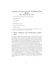
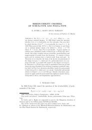
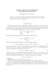
The soluti<strong>on</strong> (6.2) imitates a ‘vortex’ in a cavity, the center of the vortex is at the<br />
point with the coordinates x 01R 1 log´exp´R y 01R 2 log´exp´R 2µ·1µ2µ0512. Thus, the soluti<strong>on</strong><br />
1µ·1µ2µ0842<br />
has a boundary layer<br />
near the right boundary of the domain (see [2]). Figure 1 illustrates the distributi<strong>on</strong><br />
of the velocity vector (left) and the pressure field (right). The calculati<strong>on</strong> results <strong>for</strong><br />
R 142985R 201 are presented in Tables 3 and 4. Table 3 c<strong>on</strong>tains the calculati<strong>on</strong><br />
results <strong>for</strong> the <str<strong>on</strong>g>method</str<strong>on</strong>g> of orthog<strong>on</strong>alizati<strong>on</strong>, Table 4 c<strong>on</strong>tains the results <strong>for</strong><br />
the stabilized scheme. Since large gradients of velocity and pressure appear in the<br />
boundary layer, the number of iterati<strong>on</strong>s necessary <strong>for</strong> the c<strong>on</strong>vergence is greater<br />
than in the previous example. As in the first example, the soluti<strong>on</strong> obtained with<br />
ε10 8 coincides with the soluti<strong>on</strong> obtained <strong>for</strong> the same approximate problem<br />
with ε10 10 up to eight digits after the decimal point.<br />
The results presented in Tables 1– 4 dem<strong>on</strong>strate the sec<strong>on</strong>d order of c<strong>on</strong>vergence<br />
<strong>for</strong> velocity and the same order <strong>for</strong> pressure using orthog<strong>on</strong>alizati<strong>on</strong>,<br />
and slightly worse using stabilizati<strong>on</strong>. Moreover, the number of iterati<strong>on</strong>s <strong>for</strong> the<br />
<str<strong>on</strong>g>Uzawa</str<strong>on</strong>g>–CG <str<strong>on</strong>g>method</str<strong>on</strong>g> with the stabilized scheme practically does not depend <strong>on</strong> the<br />
mesh size. The results of both <str<strong>on</strong>g>method</str<strong>on</strong>g>s are close; in the case of orthog<strong>on</strong>alizati<strong>on</strong><br />
they are slightly better. Un<strong>for</strong>tunately, in the three-dimensi<strong>on</strong>al case the <str<strong>on</strong>g>method</str<strong>on</strong>g> of<br />
orthog<strong>on</strong>alizati<strong>on</strong> is not efficient because of the growth of the kernel dimensi<strong>on</strong>, but<br />
the stabilizati<strong>on</strong> <str<strong>on</strong>g>method</str<strong>on</strong>g> remains applicable.
<str<strong>on</strong>g>Uzawa</str<strong>on</strong>g> <str<strong>on</strong>g>method</str<strong>on</strong>g> <strong>on</strong> <strong>semi</strong>-<strong>staggered</strong> <strong>grids</strong> 557<br />
1<br />
velocity field<br />
0.8<br />
4<br />
y<br />
0.6<br />
z<br />
2<br />
0<br />
0.4<br />
−2<br />
0.2<br />
−4<br />
1<br />
0.5<br />
0.5<br />
1<br />
0 0.2 0.4 0.6 0.8 1<br />
x<br />
Figure 1. The velocity vector (left) and pressure (right) <strong>for</strong> example (6.2).<br />
y<br />
0<br />
x<br />
Table 3.<br />
C<strong>on</strong>vergence of the difference soluti<strong>on</strong> and the number of iterati<strong>on</strong>s, example (6.2), orthog<strong>on</strong>alizati<strong>on</strong>.<br />
h<br />
e hL 2<br />
e hL 2<br />
e 2hL 2<br />
log 2e hL 2<br />
e 2hL 2<br />
r hL 2<br />
r hL 2<br />
r 2hL 2<br />
log 2r hL 2<br />
r 2hL 2<br />
#it #it<br />
132 73731¢10 3 41343 20476 13453¢10 1 43257 21129 14 18<br />
164 17834¢10 3 40346 20124 31101¢10 2 40813 20290 14 19<br />
1128 44203¢10 4 40087 20031 76204¢10 3 40203 20073 14 19<br />
1256 11027¢10 4 40022 20008 18955¢10 3 40051 20018 15 19<br />
1512 27552¢10 5 47327¢10 4 15 19<br />
Table 4.<br />
C<strong>on</strong>vergence of the difference soluti<strong>on</strong> and the number of iterati<strong>on</strong>s, example (6.2), stabilizati<strong>on</strong>.<br />
h<br />
e hL 2<br />
e hL 2<br />
e 2hL 2<br />
log 2e hL 2<br />
e 2hL 2<br />
r hL 2<br />
r hL 2<br />
r 2hL 2<br />
log 2r hL 2<br />
r 2hL 2<br />
#it #it<br />
132 82125¢10 3 40081 20029 14631¢10 1 34115 17704 20 23<br />
164 20490¢10 3 39559 19840 42889¢10 2 30684 16175 20 24<br />
1128 51796¢10 4 39663 19878 13977¢10 2 29778 15742 21 24<br />
1256 13059¢10 4 39808 19931 46940¢10 3 29234 15476 21 24<br />
1512 32805¢10 5 16057¢10 3 21 24
558 L. V. Muravleva and E. A. Muravleva<br />
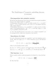
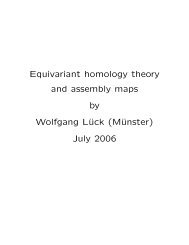
Figure 2. The velocity profile <strong>for</strong> example (6.3) with σ s02.<br />
6.3. Flow between<br />
v <br />
plates (viscoplastic medium)<br />
There are few analytic soluti<strong>on</strong>s <strong>for</strong> the models of a viscoplastic medium. C<strong>on</strong>sider<br />
<strong>on</strong>e of them, a flow<br />
<br />
between fixed<br />
sµ2<br />
plates (the plane Poiseuille flow):<br />
u0p<br />
1<br />
8´1 2σ ´1 2σ s 2xµ2℄0xx 1<br />
1<br />
2σ x 1xx 2 (6.3)<br />
8´1 1<br />
8´1 2σ sµ2 y·1<br />
2<br />
where<br />
s x 11<br />
σ sx 21<br />
(6.4)<br />
2 2·σ If σ s0, then we have not a viscoplastic medium, but a viscous liquid possessing<br />
a parabolic velocity profile. In the range 0σ s12 the velocity profile has the<br />
following <strong>for</strong>m: the interval x¾x 1x 2℄corresp<strong>on</strong>ds to the rigid z<strong>on</strong>e whose points<br />
all move at the same velocity´1 2σ sµ28, in the lateral intervals x¾0x 1µand<br />
x¾´x 21℄ade<strong>for</strong>med medium moves. For σ s02 the velocity profile is presented<br />
in Fig. 2. The greater σ s , the wider is the rigid z<strong>on</strong>e and the lower is the velocity.<br />
For σ s12 we have v0, i.e., the whole domain <strong>for</strong>ms a rigid fixed z<strong>on</strong>e.<br />
The dependence of the number of external iterati<strong>on</strong>s necessary <strong>for</strong> the c<strong>on</strong>vergence<br />
of <str<strong>on</strong>g>Uzawa</str<strong>on</strong>g> <str<strong>on</strong>g>method</str<strong>on</strong>g> (5.2)–(5.3) <strong>for</strong> µ1σ s02, is presented in Table 5.<br />
According to estimate (4.13), the sufficient c<strong>on</strong>diti<strong>on</strong> <strong>for</strong> the c<strong>on</strong>vergence of the algorithm<br />
is 0r4µσ s 2 . The first row presents the number of iterati<strong>on</strong>s in the<br />
calculati<strong>on</strong> <strong>on</strong> a uni<strong>for</strong>m grid with the mesh size 140, the sec<strong>on</strong>d row corresp<strong>on</strong>ds<br />
to the size 164. For r4µσ s100 2 the <str<strong>on</strong>g>method</str<strong>on</strong>g> c<strong>on</strong>verges, and in this case the<br />
value r999 requires 1024 and 1385 iterati<strong>on</strong>s, respectively. For r100 (and<br />
1µ2℄1<br />
´2x 2σ s sx1<br />
2·σ
<str<strong>on</strong>g>Uzawa</str<strong>on</strong>g> <str<strong>on</strong>g>method</str<strong>on</strong>g> <strong>on</strong> <strong>semi</strong>-<strong>staggered</strong> <strong>grids</strong> 559<br />
Table 5.<br />
The dependence of the number of iterati<strong>on</strong>s <strong>on</strong> the parameter r, example (6.3)<br />
with σ s02.<br />
h 1 10 20 30 40 50 60 70 80 90 99 99.5 99.9<br />
140 331 164 106 80 65 55 48 43 39 36 101 204 1024<br />
164 306 190 125 97 80 69 61 56 317 325 332 351 1385<br />
Table 6.<br />
The c<strong>on</strong>vergence of the difference soluti<strong>on</strong> and the number of iterati<strong>on</strong>s, example (6.3).<br />
h<br />
e hL 2<br />
e hL 2<br />
e 2hL 2<br />
log 2e hL 2<br />
e 2hL 2<br />
#it<br />
e hL 2<br />
e hL 2<br />
e 2hL 2<br />
log 2e hL 2<br />
e 2hL 2<br />
120 6079¢10 6 42289 20803 28 1668¢10 5 39311 19749 52<br />
140 1437¢10 6 34208 17743 48 4244¢10 6 36274 18589 98<br />
180 4202¢10 7 27754 14727 88 1170¢10 6 26495 14057 191<br />
1160 1514¢10 7 165 4416¢10 7 346<br />
#it<br />
greater) we get divergence. Thus, restricti<strong>on</strong> (4.13) related to the c<strong>on</strong>tinuous problem<br />
is c<strong>on</strong>firmed in numerical calculati<strong>on</strong>s. As can be seen, <strong>for</strong> small r the c<strong>on</strong>vergence<br />
is sufficiently slow, and <strong>for</strong> an r close to the right boundary of the interval<br />
it also becomes slower. The best c<strong>on</strong>vergence is observed <strong>for</strong> the values from the<br />
middle of the interval. Under a fixed r, the number of iterati<strong>on</strong>s increases <strong>for</strong> a finer<br />
grid.<br />
Table 6 presents the values of the velocity error norm e hvΩ 1<br />
v h in the grid<br />
analogue of the L 2 -norm <strong>for</strong> example (6.3). The left half of the table corresp<strong>on</strong>ds to<br />
the yield stress σ s02, r60, the right <strong>on</strong>e corresp<strong>on</strong>ds to σ s03, r20. The<br />
Stokes problem in internal iterati<strong>on</strong>s was solved by the orthog<strong>on</strong>alizati<strong>on</strong> <str<strong>on</strong>g>method</str<strong>on</strong>g>.<br />
The number of external iterati<strong>on</strong>s in the <str<strong>on</strong>g>Uzawa</str<strong>on</strong>g> <str<strong>on</strong>g>method</str<strong>on</strong>g> corresp<strong>on</strong>ds to the stopping<br />
criteri<strong>on</strong> ε10 3 .<br />
6.4. Driven cavity problem (viscoplastic medium)<br />
There are two test problems <strong>for</strong> numerical algorithms solving viscoplastic problems:<br />
a flow in a pipe (the Western authors sometimes refer to it as Mosolov’s problem)<br />
and a flow in a cavity. The first problem is simpler; its equivalent problem <strong>for</strong> a viscous<br />
fluid is reduced to the soluti<strong>on</strong> of the Poiss<strong>on</strong> equati<strong>on</strong> and is of great interest<br />
<strong>for</strong> mechanics. There<strong>for</strong>e, it is solved especially often [17, 19, 21, 24]. The sec<strong>on</strong>d<br />
problem is the best known test in computati<strong>on</strong>al hydrodynamics <strong>for</strong> the Stokes<br />
problem. It also becomes the test <strong>for</strong> a <strong>Bingham</strong> medium [6, 7, 10, 15, 22, 27] and<br />
c<strong>on</strong>sists in the following: let Ω´01µ2 , f0, the boundary c<strong>on</strong>diti<strong>on</strong>s be given in
560 L. V. Muravleva and E. A. Muravleva<br />
‖v‖ L2<br />
0.2<br />
0.15<br />
5<br />
3<br />
2<br />
τ s<br />
= 1<br />
0.1<br />
0.05<br />
0 0.02 0.04 0.06 0.08<br />
t<br />
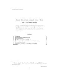
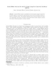
Figure 3. The velocity norm<br />
B´xµ:´0<br />
and stop time.<br />
the following way:<br />
B<br />
x¾ΓÒΓ B<br />
v<br />
16´x2 1´1 x 1µ2µ0x¾Γ where Γ Bxx´x 2µ0x<br />
1x 11x 21is the moving upper boundary. This<br />
choice of the n<strong>on</strong>zero horiz<strong>on</strong>tal velocity comp<strong>on</strong>ent corresp<strong>on</strong>ds to the so-called<br />
regularized driven cavity problem.<br />
Unsteady flows <strong>for</strong> viscoplastic media have been little studied, <strong>on</strong>ly <strong>on</strong>e-dimensi<strong>on</strong>al<br />
problems were usually c<strong>on</strong>sidered [4]. In recent papers [20, 21], numerical<br />
simulati<strong>on</strong>s of the <strong>unsteady</strong> flow of a <strong>Bingham</strong> medium were per<strong>for</strong>med <strong>for</strong> channels<br />
of various cross-secti<strong>on</strong>s. An <strong>unsteady</strong> problem of the flow in a cavity was<br />
c<strong>on</strong>sidered in [6, 7] based <strong>on</strong> the splitting <str<strong>on</strong>g>method</str<strong>on</strong>g> [13] with the use of FEM. In [7],<br />
rigid z<strong>on</strong>es were obtained <strong>for</strong> the steady driven cavity problem, and the graph of the<br />
dependence of the velocity vector norm <strong>on</strong> time was presented <strong>for</strong> the process of the<br />
start-up of the flow (reaching the stati<strong>on</strong>ary state) and subsequent cessati<strong>on</strong> of the<br />
flow. Let us describe these modes in more detail:<br />
B<br />
(1) Start-up of the flow: starting from the rest (v´0µ0) under the acti<strong>on</strong> of<br />
the instantaneously applied moti<strong>on</strong> of the ‘cover’ of the cavity (v´tµΓv ) the<br />
medium accelerates in the course of the time interval´0t 1℄, and the flow actually<br />
reaches the steady state;<br />
(2) Cessati<strong>on</strong> of the flow: from the state reached by the time moment tt 1 the<br />
medium comes to a halt because the moti<strong>on</strong> of the cover is ‘blocked’: <strong>for</strong> tt 1 we<br />
have v B´xµ0. The important qualitative peculiarity of the problems c<strong>on</strong>cerning<br />
the <strong>unsteady</strong> flows of viscoplastic media is the finiteness of the damping time of the<br />
moti<strong>on</strong> in the absence of external <strong>for</strong>ces [6]. This is a fundamental distincti<strong>on</strong> from<br />
the corresp<strong>on</strong>ding flow of a viscous liquid, which damps exp<strong>on</strong>entially in infinitely<br />
l<strong>on</strong>g time.
<str<strong>on</strong>g>Uzawa</str<strong>on</strong>g> <str<strong>on</strong>g>method</str<strong>on</strong>g> <strong>on</strong> <strong>semi</strong>-<strong>staggered</strong> <strong>grids</strong> 561<br />
(a)<br />
(b)<br />
(c)<br />
(d)<br />
s<br />
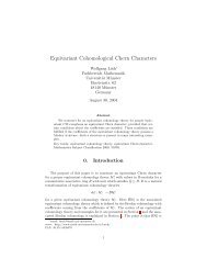
Figure 4. Development of rigid z<strong>on</strong>es <strong>for</strong> τ s1: (a) t0, (b) t0004, (c) t0008, (d) t001.<br />
The graphs in Fig. 3 illustrate the dependence of the velocity vector normv hh<br />
<strong>on</strong> time. The results are presented <strong>for</strong> τ s1´t 1006µτ s2´t 10055µτ 3´t 1005µτ s5´t 10045µ. It is easy to see that the medium stops in a finite<br />
time interval. The curve <strong>for</strong> τ s1 is identical to Fig. 11 from [7].<br />
It was noted in a classic m<strong>on</strong>ograph (see [10]) that ‘naturally, the problem <strong>on</strong> determinati<strong>on</strong><br />
of rigid z<strong>on</strong>es is of most interest in numerical experiments’. Figures 4a–<br />
4d illustrate the evoluti<strong>on</strong> of rigid z<strong>on</strong>es in time <strong>for</strong> the stopping problem. The results<br />
are presented <strong>for</strong> µ1ρ1τ s1´σ sÔ2µ. The results were obtained <strong>on</strong><br />
a grid with the mesh size h1128 and the c<strong>on</strong>vergence criteri<strong>on</strong> ε10 4 . Rigid<br />
z<strong>on</strong>es were determined as isolinesτ hσ s (the v<strong>on</strong> Mises criteri<strong>on</strong> is applied to the<br />
discrete field τ h ). Figure 4a corresp<strong>on</strong>ds to the steady flow of a viscoplastic medium<br />
in a cavity and it is in a good agreement with the previous papers [6, 7, 15, 22, 27].<br />
Three rigid z<strong>on</strong>es are present in this flow at the initial moment corresp<strong>on</strong>ding to the<br />
steady state. One of them is located near the center of the vortex and two others lie<br />
in the bottom part of the cavity. The bottom rigid z<strong>on</strong>es gradually merge (Fig. 4b)<br />
and increase in size (Fig. 4c). The central rigid z<strong>on</strong>e sinks and also increases. In the<br />
course of time (sufficiently so<strong>on</strong>) three additi<strong>on</strong>al rigid z<strong>on</strong>e appear in the upper corners<br />
and above the central rigid z<strong>on</strong>e. Some symmetry is quite natural here, because
562 L. V. Muravleva and E. A. Muravleva<br />
the upper boundary of the domain becomes fixed. Further increase and merging of<br />
rigid z<strong>on</strong>es progresses. Figure 4d illustrates the situati<strong>on</strong> shortly be<strong>for</strong>e the complete<br />
stop of the flow: <strong>on</strong>ly a thin band of the moving medium remains between the outer<br />
(adjacent to the boundary) and the inner rigid z<strong>on</strong>es. The appearance of additi<strong>on</strong>al<br />
rigid z<strong>on</strong>es (beside those existing in the steady state) and their further merging is<br />
the typical peculiarity of <strong>unsteady</strong> flows of viscoplastic media. A similar pattern<br />
was observed when the flow in a channel was stopped [21].<br />
7. C<strong>on</strong>clusi<strong>on</strong><br />
In this paper we justify at the functi<strong>on</strong>al level the applicati<strong>on</strong> of the <str<strong>on</strong>g>Uzawa</str<strong>on</strong>g> <str<strong>on</strong>g>method</str<strong>on</strong>g><br />
<strong>for</strong> the soluti<strong>on</strong> of <strong>unsteady</strong> viscoplastic problems (without c<strong>on</strong>vective terms). Estimates<br />
of the c<strong>on</strong>vergence interval are obtained <strong>for</strong> the iterative parameter of the<br />
<str<strong>on</strong>g>Uzawa</str<strong>on</strong>g> <str<strong>on</strong>g>method</str<strong>on</strong>g>. In this case the restricti<strong>on</strong> relating to the c<strong>on</strong>tinuous problem practically<br />
coincides with the c<strong>on</strong>vergence interval obtained numerically in the finitedimensi<strong>on</strong>al<br />
problem. The <str<strong>on</strong>g>method</str<strong>on</strong>g> has been implemented in a rectangular domain<br />
by a difference scheme <strong>on</strong> <strong>semi</strong>-<strong>staggered</strong> <strong>grids</strong>. Numerical experiments c<strong>on</strong>firm<br />
the efficiency of the proposed approach. The evoluti<strong>on</strong> of rigid z<strong>on</strong>es <strong>for</strong> a plane<br />
<strong>unsteady</strong> viscoplastic problem has been obtained (to best of our knowledge) <strong>for</strong> the<br />
first time and is of great interest <strong>for</strong> applied problems. In future we expect to present<br />
a more detailed justificati<strong>on</strong> of the applicati<strong>on</strong> of difference approximati<strong>on</strong>s and the<br />
c<strong>on</strong>vergence of the algorithm in the finite-dimensi<strong>on</strong>al case, and also to extend the<br />
results to the three-dimensi<strong>on</strong>al <strong>unsteady</strong> case.<br />
Acknowledgement<br />
The authors are sincerely grateful to V. I. Agoshkov <strong>for</strong> useful comments.<br />
References<br />
1. M. Benzi, G. H. Golub, and J. Liesen, Numerical soluti<strong>on</strong> of saddle point problems. Acta Numerica<br />
(2005) 14, 1–137.<br />
2. S. Berr<strong>on</strong>e, Adaptive discretizati<strong>on</strong> of the Navier Stokes equati<strong>on</strong>s by stabilized finite element<br />
<str<strong>on</strong>g>method</str<strong>on</strong>g>s. Comp. Meth. Appl. Mech. Engrg. (2001) 190, 4435–4455.<br />
3. P. B. Bochev, C. R. Dohrmann, and M. D. Gunzburger, Stabilizati<strong>on</strong> of low-order mixed finite<br />
elements <strong>for</strong> the Stokes equati<strong>on</strong>s. SIAM J. Numer. Anal. (2006) 44, 82–101.<br />
4. M. Chatzimina, C. Xenoph<strong>on</strong>tos, G. C. Georgiou, I. Argyropaidas, and E. Mitsoulis, Cessati<strong>on</strong><br />
of annular Poiseuille flows of <strong>Bingham</strong> plastics. J. N<strong>on</strong>-Newt<strong>on</strong>ian Fluid Mech. (2007) 142,<br />
135–142.<br />
5. E. V. Chizh<strong>on</strong>kov, Relaxati<strong>on</strong> Methods <strong>for</strong> Saddle Point Problems. Moscow, INM RAS, 2002<br />
(in Russian).<br />
6. E. J. Dean and R. Glowinski, Operator-splitting <str<strong>on</strong>g>method</str<strong>on</strong>g>s <strong>for</strong> the simulati<strong>on</strong> of <strong>Bingham</strong> viscoplastic<br />
flow. Chin. Ann. Math. (2002) 23, 187–204.
<str<strong>on</strong>g>Uzawa</str<strong>on</strong>g> <str<strong>on</strong>g>method</str<strong>on</strong>g> <strong>on</strong> <strong>semi</strong>-<strong>staggered</strong> <strong>grids</strong> 563<br />
7. E. J. Dean, R. Glowinski, and G. Guidob<strong>on</strong>i, On the numerical simulati<strong>on</strong> of <strong>Bingham</strong> viscoplastic<br />
flow: Old and New results. J. N<strong>on</strong>-Newt<strong>on</strong>ian Fluid Mech. (2007) 142, 36–62.<br />
8. G. Duvaut and J.-L. Li<strong>on</strong>s, Inequalities in Mechanics and Physics. Springer, New York, 1976.<br />
9. I. Ekeland and R. Temam, C<strong>on</strong>vex analysis and variati<strong>on</strong>al problems. North-Holland, Amsterdam,<br />
1976.<br />
10. R. Glowinski, J.-L.Li<strong>on</strong>s, and R. Tremolier‘es, Numerical Analysis of Variati<strong>on</strong>al Inequalities.<br />
North Holland, Amsterdam, 1981.<br />
11. A. A. Il’yushin, De<strong>for</strong>mati<strong>on</strong> of viscoplastic body. Uchenye Zapiski MGU. Mekhanika (1940)<br />
39, 3–81 (in Russian).<br />
12. A. V. Lapin, Introducti<strong>on</strong> into the Theory of Variati<strong>on</strong>al Inequalities. KSU publishing house,<br />
Kazan, 1981 (in Russian).<br />
13. G. I. Marchuk, Splitting Methods. Nauka, Moscow, 1988 (in Russian).<br />
14. G. I. Marchuk and V. I. Agoshkov, Introducti<strong>on</strong> to Projecti<strong>on</strong>-grid Methods. Nauka, Moscow,<br />
1981 (in Russian).<br />
15. E. Mitsoulis and Th. Zisis, Flow of <strong>Bingham</strong> plastics in a lid-driven cavity. J. N<strong>on</strong>-Newt<strong>on</strong>ian<br />
Fluid Mech. (2001) 101, 173–180.<br />
16. P. P. Mosolov and V. P. Myasnikov, Mechanics of Rigid Plastic Bodies. Nauka, Moscow, 1981<br />
(in Russian).<br />
17. M. A. Moyers-G<strong>on</strong>zalez and I. A. Frigaard, Numerical soluti<strong>on</strong> of duct flows of multiple viscoplastic<br />
fluids. J. N<strong>on</strong>-Newt<strong>on</strong>ian Fluid Mech. (2004) 122, 227–241.<br />
18. E. A. Muravleva, On the kernel of the discrete gradient operator. Numer. Meth. Prog. (2008) 9,<br />
No. 1, 97–104.<br />
19. E. A. Muravleva, Finite-difference schemes <strong>for</strong> computati<strong>on</strong> viscoplastic medium flow in channel.<br />
Math. Model. Comp. Simulati<strong>on</strong>s (2008) 20, No. 12, 76–88.<br />
20. E. A. Muravleva, The problem of stopping the flow of a viscoplastic medium in a channel.<br />
Moscow Univ. Mech. Bulletin (2009) 64, No. 1, 25–28.<br />
21. E. A. Muravleva and L. V. Muravleva, Unsteady flows of viscoplastic medium in channels. Mech.<br />
Solids (2009) 44, No. 5, 792–812.<br />
22. E. A. Muravleva and M. A. Olshanskii, Two finite-difference schemes <strong>for</strong> calculati<strong>on</strong> of <strong>Bingham</strong><br />
fluid flows in a cavity. Russ. J. Numer. Anal. Math. Modelling (2008) 23, No. 6, 615–634.<br />
23. E. A. Muravleva, Analysis of Scheme <strong>on</strong> Semi-<strong>staggered</strong> Grids <strong>for</strong> Stokes Problem. Preprint of<br />
ICM, H<strong>on</strong>g K<strong>on</strong>g (2009) (submitted).<br />
24. N. Roquet and P. Saramito, An adaptive finite element <str<strong>on</strong>g>method</str<strong>on</strong>g> <strong>for</strong> viscoplastic fluid flows in<br />
pipes. Comp. Meth. Appl. Mech. Engrg. (2001) 190(40), 5391–5412.<br />
25. A. G. Churbanov, A. N. Pavlov, and P. N. Vabishchevich, Operator-splitting <str<strong>on</strong>g>method</str<strong>on</strong>g> <strong>for</strong> incompressible<br />
Navier–Stokes equati<strong>on</strong>s <strong>on</strong> n<strong>on</strong>-<strong>staggered</strong> <strong>grids</strong>. Part I: First-order schemes. Int. J.<br />
Numer. Meth. Fluids (1995) 21, 617–640.<br />
26. F. P. Vasiliev, Optimizati<strong>on</strong> Methods. Factorial Press, Moscow, 2002.<br />
27. D. Vola, L. Boscardin, and J. C. Latche, Laminar <strong>unsteady</strong> flows of <strong>Bingham</strong> fluids: a numerical<br />
strategy and some benchmark results. J. Comp. Phys. (2003) 187, 441–456.