Actor Critic Method: Maze Example - FIAS

Actor Critic Method:
Maze Example
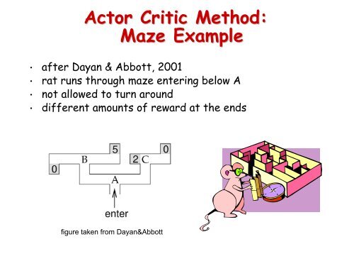
• after Dayan & Abbott, 2001
• rat runs through maze entering below A
• not allowed to turn around
• different amounts of reward at the ends
figure taken from Dayan&Abbott

Solving the Maze Problem
Assumptions:
• state is fully observable (in contrast to only partially
observable), i.e. the rat knows exactly where it is at any
time
• actions have deterministic consequences (in contrast to
probabilistic)
Idea: maintain and improve a stochastic policy which
determines the action at each decision point (A,B,C)
using action values and softmax decision rule
Actor Critic Learning:
• critic: use temporal difference learning to predict
future rewards from A,B,C if current policy is followed
• actor: maintain and improve the policy

Actor-Critic Method
Policy
Agent
Actor
state
Critic
Value
Function
TD
error
action
reward
Environment

Formal Setup
• state variable u (is rat at A,B, or C)
• action value vector Q(u) describing policy (left/right)
• softmax rule assigns probability of action a based on
action values
• immediate reward for taking action a in state u: r a (u)
• expected future reward for starting in state u and
following current policy: v(u) (state value function)
• The rat estimates this with weights w(u)
critic
v
actor
Q L Q R
figure taken from Dayan&Abbott
w(A)
A B C
A B C

Policy Iteration
• Two Observations:
• We need to estimate the values of the states, but these depend
on the rat’s current policy.
• We need to chose better actions, but what action appears
“better” depends on the values estimated above.
• Idea (policy iteration): just iterate the two processes
• Policy Evaluation (critic): estimate state value function (weights
w(u)) using temporal difference learning.
• Policy Improvement (actor): improve action values Q(u) based
on estimated state values.

Policy Evaluation
Initially, assume all action values are 0, i.e. left/right
equally likely everywhere. What is the value of each state
assuming there is no discounting
True value of each state can be
found by inspection:
v(B) = ½(5+0)=2.5;
v(C) = ½(2+0)=1;
v(A) = ½(v(B)+v(C))=1.75.
2.5 1
1.75
figure taken from Dayan&Abbott
How can we learn these values through online experience

Temporal Difference Learning
Idea: values of successive states are related. This is expressed
through the Bellman equation:
V
π
( s)
{ s s}
{ }
π
R s = s = E r + γV
( s )
= Eπ
t
π t 1
t+
t + 1 t
=
Deviations of estimated values of successive states from this
relation need to be corrected. Define the temporal difference
error as a (sampled) measure of such deviations:
δ
( t) r + V ( s ) 1
−V
( s )
= γ
t+ 1 t+
t
Now update the estimate of the value of the current state:
V
( s ) V ( s ) + ε[
r + V ( s ) −V
( s )]
t
← γ
t t+ 1 t+
1
t

Policy Evaluation Example
w ( u)
→ w(
u) + εδ with є=0.5 and δ = ( u)
+ v(
u')
− v(
u)
r a
Thick lines are running average of weight values;
figure taken from Dayan&Abbott

Note: Sutton and
Barto book uses “p”
for action
preferences
Q
a'
δ =
r a
Policy Improvement
(using a so-called direct actor rule)
( u)
→ Qa'
( u)
+ ε ( δ
aa'
− p(
a';
u))
δ
( u)
+ v(
u')
− v(
u)
positive if a’ was chosen, else negative
, where
positive if outcome better
than expected, else negative
p(a ’;u) is the softmax probability of choosing action a’ in
state u as determined by Q a’ (u)
This term is not strictly necessary but has the advantage
that actions which are already chosen with very high
probability only increase their Q value very slowly

Q
a'
δ =
( u)
→ Qa'
( u)
+ ε ( δ
aa'
− p(
a';
u))
δ
r a
( u)
+ v(
u')
− v(
u)
positive if a’ was chosen, else negative
, where
positive if outcome better
than expected, else negative
Example: consider starting out from random policy and assume
state value estimates w(u) are accurate. Consider u=A:
Rat will increase probability of
going left in location A because:
2.5 1
1.75
δ = 0 + v(
B)
− v(
A)
= 0.75
δ = 0 + v(
C)
− v(
A)
= −0.75
if left turn
if right turn

Policy Improvement Example
•learning rate є=0.5
• inverse temperature β=1
figures taken from Dayan&Abbott