The Locally Most Powerful Invariant Test for ... - COMONSENS

2012 IEEE 7th Sensor Array and Multichannel Signal Processing Workshop (SAM)
The Locally Most Powerful Invariant Test
for Detecting a Rank-P Gaussian Signal
in White Noise
David Ramírez
Dept. of Electrical Engineering
and Information Technology
Universität Paderborn
Paderborn, Germany
Email: david.ramirez@sst.upb.de
Jorge Iscar, Javier Vía
and Ignacio Santamaria
Dept. of Communications Engineering
University of Cantabria
Santander, Spain
Email: {jorge, jvia, nacho}@gtas.dicom.unican.es
Louis L. Scharf
Depts. of Mathematics and Statistics
Colorado State University
Fort Collins, USA
Email: scharf@engr.colostate.edu
Abstract—Spectrum sensing has become one of the main
components of a cognitive transmitter. Conventional detectors
suffer from noise power uncertainties and multiantenna detectors
have been proposed to overcome this difficulty, and to improve
the detection performance. However, most of the proposed
multiantenna detectors are based on non-optimal techniques,
such as the generalized likelihood ratio test (GLRT), or even
heuristic approaches that are not based on first principles. In this
work, we derive the locally most powerful invariant test (LMPIT),
that is, the optimal invariant detector for close hypotheses, or
equivalently, for a low signal-to-noise ratio (SNR). The traditional
approach, based on the distributions of the maximal invariant
statistic, is avoided thanks to Wijsman’s theorem, which does
not need these distributions. Our findings show that, in the low
SNR regime, and in contrast to the GLRT, the additional spatial
structure imposed by the signal model is irrelevant for optimal
detection. Finally, we use Monte Carlo simulations to illustrate
the good performance of the LMPIT.
Index Terms—Cognitive Radio, locally most powerful invariant
test (LMPIT), multi antenna spectrum sensing, Wijsman’s
theorem.
I. INTRODUCTION
The cognitive radio (CR) paradigm is a new technology that
aims to improve spectrum usage and alleviate the apparent
scarcity of resources [1]. The main idea is based on the
observation that there are temporally and/or geographically
unused bands. Basically, CR relies on the opportunistic access
of non-licensed users (secondary users) to these unused bands,
avoiding interfering with rightful license owners. This translates
into the need for powerful spectrum sensing (detection
of primary activity) in CR networks. However, as might be
expected, this is a challenging task due to shadowing and
fading phenomena, as well as to the low SNR conditions.
To obtain the desired performance in such challenging
environments, spectrum sensing techniques may exploit certain
features of the signals, such as cyclostationarity and/or the
presence of pilots. However, those approaches usually require
a level of synchronization not achievable in most practical
scenarios. Hence, asynchronous detectors are of interest, the
most popular being the energy detector (ED). Nevertheless, in
the presence of noise power uncertainties, the performance of
the energy detector is severely degraded [2]. To overcome this
problem, and improve the detection performance, multiantenna
detectors are typically considered. These detectors are usually
based on the generalized likelihood ratio test (see [3] and
references therein), or heuristic approaches. However, it is well
known that, in general, these techniques lead to suboptimal
tests.
In this work, we derive the locally most powerful invariant
test (LMPIT) for the typical signal-plus-noise model, usually
found in communication systems. Hence, we obtain the optimal
invariant detector in the low signal-to-noise ratio (SNR)
regime. The derivation of the LMPIT usually becomes a
complicated task because we need to derive the distributions
of the maximal invariant. However, using Wijsman’s theorem
[4], [5], we can calculate the ratio of the distributions of the
maximal invariant statistic without deriving the distributions,
and even without obtaining the maximal invariant statistic. On
the other hand, we must point out that the LMPIT for a closely
related problem was obtained in [6], where the author used
the (more complicated) conventional approach for deriving the
LMPIT.
II. SYSTEM MODEL
We consider the problem of spectrum sensing using multiantenna
spectrum monitors. The problem is formulated in
such a way that it does not require prior knowledge about
the primary signals, the wireless channel, nor the noise processes
(beyond spatial independence). We consider P signals,
which may be generated by a P -antenna transmitter,
P single-antenna users, or any combination, impinging on
an L-antenna spectrum monitor. At the receiver, the signals
are downconverted and sampled at the Nyquist rate, without
synchronization with any potentially present primary signal.
Taking this into account, the spectrum sensing problem is
formulated as
H 1 : x[n] = Hs[n] + v[n], n = 0, . . . , M − 1
H 0 : x[n] = v[n], n = 0, . . . , M − 1
(1)
978-1-4673-1071-0/12/$31.00 ©2012 IEEE 501

where s[n] = [s 1 [n], . . . , s P [n]] T is the transmitted signal,
H ∈ C L×P is the wireless channel, and v[n] =
[v 1 [n], . . . , v L [n]] T is the additive noise vector, which is
assumed to be zero-mean circular complex Gaussian, independent
of s[n], and spatially and temporally white. Moreover,
the transmitted signal is considered temporally and spatially
white, and the channel is flat fading. Under these assumptions,
the covariance matrix of the measurements is, for all n,
H 1 : R = HH H + σ 2 I,
H 0 : R = σ 2 I,
where σ 2 is the noise power and R = E[x[n]x H [n]].
Before proceeding, we assume that s[n] is zero-mean,
circular complex Gaussian, which will result in tractable
analysis and useful detectors, and can also be seen as a worst
case distribution [7]. Therefore, the detection problem in (2)
becomes
H 1 : x[n] ∼ CN ( 0, HH H + σ 2 I ) ,
H 0 : x[n] ∼ CN ( 0, σ 2 I ) ,
where CN (µ, R) stands for the complex circular Gaussian
distribution with mean µ and covariance matrix R. Hence,
the spectrum sensing problem has been formulated as a test
for the covariance structure of the received measurements.
Specifically, under H 0 the covariance matrix is proportional
to the identity matrix, whereas, under H 1 , it is the sum of a
rank-P matrix and the noise covariance matrix.
III. PREVIOUS WORK
A. Generalized Likelihood Ratio Test (GLRT)
The detection problem in (3) is a composite test, that
is, the likelihoods depend on unknown parameters. Previous
approaches to this problem in the context of spectrum sensing
are based on the well-known generalized likelihood ratio test
(GLRT), which, basically, obtains the likelihood ratio with the
unknown parameters replaced by their maximum likelihood
(ML) estimates. In particular, for the test given in (3), and
considering M independent and identically distributed (i.i.d.)
samples of x[n], the generalized likelihood ratio (GLR) is
given by
max p ( X; σ 2 I )
σ
G =
2 >0
max p (X; R 1 ) ,
R 1=HH H +σ 2 I,
σ 2 >0
where the likelihood is
1
[ ( )]
p (X; R) =
π LM |R| M exp −M tr R −1 ˆR ,
with |·| and tr (·) denoting the determinant and the trace of
a matrix, respectively. The data matrix is given by X =
[ x[0], . . . , x[M − 1]
]
and ˆR = XX H /M is the sample
covariance matrix. Finally, the test is obtained by comparing
the GLR with a threshold. In [3], it was shown that the GLRT
(2)
(3)
depends on the rank P . For P ≥ L − 1, the test becomes the
well known test for sphericity, and the GLRT is given by [8]
⎡( ∏L 1/L
⎤
i=1 i) λ
⎢
log G = log ⎣
1
L
∑ L
i=1 λ i
⎥
⎦ H0
≷ η,
H 1
where λ i is the i-th eigenvalue of ˆR. On the contrary, for
P < L − 1, the GLRT becomes [3]
⎢
log G = L log ⎣
⎡( ∏L 1/L
⎤
i=1 i) λ
∑
1 L
L i=1 λ i
⎡
⎢
− (L − P ) log ⎣
⎥
⎦
( ∏L 1/(L−P )
⎤
i=P +1 i) λ
1
L−P
∑ L
i=P +1 λ i
B. Locally Most Powerful Invariant Test (LMPIT)
⎥
⎦ H0
≷ η.
H 1
Despite its simplicity, the GLRT does not have any optimality
property and, in fact, its performance might be poor
when the sample size is small. Therefore, other detectors have
been considered for dealing with composite hypotheses. The
optimal test (uniformly most powerful test) does not exist in
general, because the likelihood ratio depends on the unknown
parameters. One possible way to avoid this dependence is
restricting ourselves to the class of invariant detectors [9]. In
this way we obtain the optimal test among those invariant,
that is, the uniformly most powerful invariant test (UMPIT).
However, when the UMPIT does not exist, we can still derive
an optimal test, under the assumption of close hypotheses, i.e.,
the locally most powerful invariant test (LMPIT).
The typical approach for deriving the LMPIT is [9]: (i)
identify the invariances of the problem and describe them
as a group of transformations, (ii) find the maximal invariant
statistic, (iii) derive the distribution of the maximal invariant
statistic under both hypotheses, (iv) calculate the ratio of the
distributions of the maximal invariant statistic, and (v) apply
a Taylor’s expansion of the likelihood ratio. 1 This approach
was used in [6] to derive the LMPIT for the sphericity test
H 1 : x[n] ∼ CN (0, R) ,
H 0 : x[n] ∼ CN ( 0, σ 2 I ) ,
with R only constrained to be a positive definite matrix. In
particular, the LMPIT is given by
where
L = ‖ ˆ˜R‖ 2
F
H 1
≷
H 0
η, (4)
ˆR ˆ˜R = ( ). (5)
tr ˆR
1 Step (v) is only necessary if the likelihood ratio depends on the unknown
parameters. Otherwise, the density ratio of the maximal invariants would
provide the uniformly most powerful invariant test (UMPIT) statistic.
502

IV. DERIVATION OF THE LMPIT: WIJSMAN’S THEOREM
The approach for deriving the LMPIT discussed in Section
III-B might be quite complicated, not only due to the need of
obtaining the distributions of the maximal invariant statistic,
but also due to the need of an explicit formulation for the
maximal invariant. Here, we use another approach, namely
Wijsman’s theorem [4], [5]. This theorem allows us to directly
obtain the maximal invariant density ratio without knowledge
of the distributions of the maximal invariant statistic, and
even without an explicit expression for the maximal invariant
statistic. Wijsman’s theorem states that, under some mild conditions,
the likelihood ratio of the maximal invariant statistic
is given by
∫
L = ∫ G p (g(y); H 1) |J g | dg
G p (g(y); H 0) |J g | dg ,
where G is the group of transformations under which the test
is invariant, |J g | denotes the absolute value of the Jacobian
of the transformations g(·) ∈ G, and dg is an invariant group
measure.
To apply Wijsman’s theorem to our problem, the first step
is to identify the problem invariances. Concretely, the group
of invariant transformations for the detection problem given
in (3) is
G = {g : x[n] → g(x[n]) = aQx[n]} ,
where a ∈ R + is a positive real number, and Q ∈ U, with U
denoting the set of unitary matrices. This means that scaling
all received signals by a common factor, or multiplying them
by a unitary matrix should not change the test. Taking into
account the invariances of our problem, Wijsman’s theorem
reads as follows
L =
∫R +
∫
U |S|2M a 2M e −a2 M tr(SQ ˆRQ H ) dQda
∫R +
∫U σ−2ML a 2M e − a2
σ 2 M tr( ˆR)
,
dQda
where S = ( HH H + σ 2 I ) −1
. Now, to obtain the LMPIT, we
have to decompose L as a function only dependent on the data
and a term not dependent on the data. Before proceeding, let
us present the following lemma.
Lemma 1: The ratio L is given (up to additive and multiplicative
constant terms not depending on data) by
where
L ∝
∫R +
∫
α = a 2 M
a 2M e −α dQda, (6)
U
L∑
k,m=1
λ k |q m,k | 2 β m .
Here λ k and β m denote the eigenvalues of ˆ˜R and S, and qm,k
is the {m, k}-th element of Q.
Proof: The proof follows directly by simply applying the
following changes of variable:
( )
a 2 → a 2 / tr ˆR , Q → U S QU HˆR,
where U S and U ˆR
are the matrices of eigenvectors of S and
ˆR, respectively.
It is easy to check that (6) is a function of the unknown
parameters, thus proving that the UMPIT does not exist, in
general. The only exception is the case of L = 2 antennas,
where the test statistic of the UMPIT [10] is given by the
largest eigenvalue of ˆ˜R, i.e., λ1 . Due to the non-existence of
the UMPIT, we consider the challenging low-SNR scenario
and derive the LMPIT. Note that in the low-SNR regime S ≈
σ −2 I ⇒ α 0 = a 2 M/σ 2 , and applying a second order Taylor
series expansion of e −α , we get
L ∝
∫R +
∫
a 2M e [ −α0 (α − α 0 ) 2 − (α − α 0 ) ] dQda,
U
Finally, the LMPIT is presented in the following result.
Theorem 1: The LMPIT is given by
L ∝
L∑
k=1
λ 2 k = ‖ ˆ˜R‖ 2
F
H 1
≷
H 0
η. (7)
Proof: Here, due to the lack of space, we only present
a sketch of the proof. First, let us consider the linear term,
which, neglecting the sign, may be rewritten as
where
∆
L∑
k,m=1
∆ =
( )
λ k β m = ∆ tr ˆ˜R tr (S) = ∆ tr (S) ,
∫R +
∫
a 2M+1 e −a2 M/σ 2 |q m,k | 2 dQda,
U
and we have taken into account that the value of the integral
does not depend on the actual indexes. Hence, we can notice
that the linear term does not depend on the data, so it can
be neglected. The quadratic term, after expanding the square,
becomes
∑
∫
λ k λ l β m β s a 2M+1 e −a2 M/σ 2 |q m,k | 2 |q s,l | 2 dQda.
k,m,l,s
R +
∫U
Now, decomposing the above summations and taking into
account that the value of the integral is the same for some
subsets of the indexes, the proof follows.
A. Further Comments
This work has derived the LMPIT using a (in our opinion)
more powerful approach, Wijsman’s theorem, whereas [6] uses
the conventional approach, requiring an explicit formulation of
the maximal invariant statistic and its distributions. Moreover,
[6] did not consider the additional spatial structure imposed by
the signal-plus-noise model. From our results, we can conclude
that in the low-SNR regime the additional structure imposed
by the signal model given in (1) and the hypothesis test in
(3) is irrelevant for optimal detection. On the contrary, it is
known that the GLRT depends on the spatial structure of the
measurements under H 1 .
503

Probability of Detection
1
0.8
0.6
0.4
0.2
GLRT
LMPIT
Probability of Detection
1
0.8
0.6
0.4
0.2
GLRT
LMPIT
0
10 20 30 40 50
L
0
−20 −15 −10 −5 0
SNR (dB)
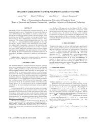
Fig. 1. Probability of detection vs. L for P = 30, M = 50, p fa = 0.1
and SNR = −6 dB.
Fig. 2. Probability of detection for p fa = 0.1, L = 40, P = 30 and
M = 40.
V. NUMERICAL RESULTS
In this section we evaluate the performance of the LMPIT
by means of Monte Carlo simulations. The noise power σ 2
is fixed during the experiment, and the entries of the channel
matrix are i.i.d. complex Gaussian random variables scaled to
achieve the same SNR per realization, with the SNR defined
as follows
SNR (dB) = 10 log 10
tr ( HH H)
Lσ 2 .
In the first experiment, we obtain the probability of detection
for a fixed false alarm probability (p fa = 0.1) and varying L,
the remaining parameters are P = 30, M = 50 samples and
SNR = −6 dB. Figure 1 shows that the performance of the
LMPIT is better than that of the GLRT, and these differences
are greater for large values 2 of L.
The second experiment analyzes the performance of the
GLRT and the LMPIT for different values of the SNR. Figure
2 shows the probability of detection for a fixed probability of
false alarm p fa = 0.1, L = 40, P = 30 and M = 40. As
expected, the performance of the LMPIT is better for these
small to moderate values of the SNR.
VI. CONCLUSIONS
We have derived the locally most powerful invariant test
(LMPIT) for a spectrum sensing problem in cognitive radio.
That is, we have obtained the optimal invariant test in the low
SNR regime. Interestingly, it turns out that the LMPIT coincides
with a previously proposed LMPIT for a closely related
problem, where the covariance matrix under the alternative is
only constrained to be positive definite. Hence, this work has
proved that the actual spatial structure of the covariance matrix
under the true hypothesis is irrelevant for optimal detection
in the low-SNR region, contrary to the GLRT, which tries
2 In a practical scenario, it is impossible to have a spectrum monitor with
such a large number of antennas, but it might be possible to use several
cooperative spectral monitors to achieve such a large number.
to exploit that information. Additionally, we have followed
an alternative approach for deriving the LMPIT, based on
Wijsman’s theorem, which overcomes the need for deriving
the distributions of the maximal invariant statistic. Finally, as
expected, simulation results illustrate the better performance
of the LMPIT for small to moderate values of the SNR.
ACKNOWLEDGMENTS
The work of J. Iscar, J. Vía and I. Santamaría was
supported by the Spanish Government, Ministerio de Ciencia
e Innovación (MICINN), under projects COSIMA
(TEC2010-19545-C04-03) and COMONSENS (CSD2008-
00010, CONSOLIDER-INGENIO 2010 Program). The work
of L. L. Scharf was supported by the Airforce Office of
Scientific Research under contract FA9550-10-1-0241.
REFERENCES
[1] J. Mitola and G. Q. Maguire Jr., “Cognitive radio: Making software
radios more personal,” IEEE Pers. Comm., vol. 6, pp. 13–18, Aug. 1999.
[2] R. Tandra and A. Sahai, “SNR walls for signal detection,” IEEE J. Sel.
Topics Signal Process., vol. 2, no. 1, pp. 4–17, Feb. 2008.
[3] D. Ramírez, G. Vázquez-Vilar, R. López-Valcarce, J. Vía, and I. Santamaría,
“Multiantenna detection of rank-P signals in cognitive radio
networks,” IEEE Trans. Signal Process., vol. 59, no. 8, pp. 3764–3774,
Aug. 2011.
[4] R. A. Wijsman, “Cross-sections of orbits and their application to
densities of maximal invariants,” in Proc. Fifth Berkeley Symp. on Math.
Stat. and Prob., vol. 1, 1967, pp. 389–400.
[5] J. Gabriel and S. Kay, “Use of Wijsman’s theorem for the ratio of
maximal invariant densities in signal detection applications,” in Asilomar
Conf. Signals, Systems and Computers, vol. 1, Nov. 2002, pp. 756 – 762.
[6] S. John, “Some optimal multivariate tests,” Biometrika, vol. 58, no. 1,
pp. 123–127, 1971.
[7] J. Villares and G. Vázquez, “The Gaussian assumption in second-order
estimation problems in digital communications,” IEEE Trans. Signal
Process., vol. 55, no. 10, pp. 4994–5002, 2007.
[8] J. Mauchly, “Significance test for sphericity of a normal n-variate
distribution,” Ann. Math. Statist., vol. 11, pp. 204–209, 1940.
[9] L. L. Scharf, Statistical Signal Processing: Detection, Estimation, and
Time Series Analysis. Addison - Wesley, 1991.
[10] O. Besson, S. Kraut, and L. L. Scharf, “Detection of an unknown rankone
component in white noise,” IEEE Trans. Signal Process., vol. 54,
no. 7, pp. 2835–2839, Jul. 2006.
504