Fast Motion Estimation With Interpolation-Free Sub ... - IEEE Xplore

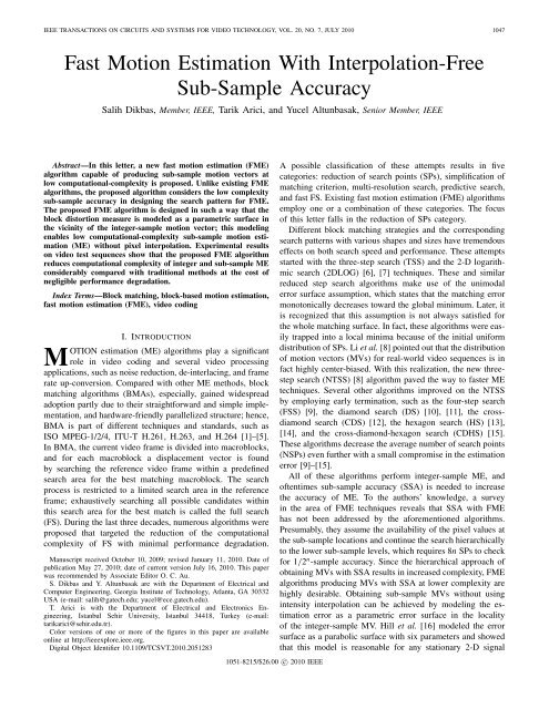
IEEE TRANSACTIONS ON CIRCUITS AND SYSTEMS FOR VIDEO TECHNOLOGY, VOL. 20, NO. 7, JULY 2010 1047
Fast Motion Estimation With Interpolation-Free
Sub-Sample Accuracy
Salih Dikbas, Member, IEEE, Tarik Arici, and Yucel Altunbasak, Senior Member, IEEE
Abstract—In this letter, a new fast motion estimation (FME)
algorithm capable of producing sub-sample motion vectors at
low computational-complexity is proposed. Unlike existing FME
algorithms, the proposed algorithm considers the low complexity
sub-sample accuracy in designing the search pattern for FME.
The proposed FME algorithm is designed in such a way that the
block distortion measure is modeled as a parametric surface in
the vicinity of the integer-sample motion vector; this modeling
enables low computational-complexity sub-sample motion estimation
(ME) without pixel interpolation. Experimental results
on video test sequences show that the proposed FME algorithm
reduces computational complexity of integer and sub-sample ME
considerably compared with traditional methods at the cost of
negligible performance degradation.
Index Terms—Block matching, block-based motion estimation,
fast motion estimation (FME), video coding
I. Introduction
MOTION estimation (ME) algorithms play a significant
role in video coding and several video processing
applications, such as noise reduction, de-interlacing, and frame
rate up-conversion. Compared with other ME methods, block
matching algorithms (BMAs), especially, gained widespread
adoption partly due to their straightforward and simple implementation,
and hardware-friendly parallelized structure; hence,
BMA is part of different techniques and standards, such as
ISO MPEG-1/2/4, ITU-T H.261, H.263, and H.264 [1]–[5].
In BMA, the current video frame is divided into macroblocks,
and for each macroblock a displacement vector is found
by searching the reference video frame within a predefined
search area for the best matching macroblock. The search
process is restricted to a limited search area in the reference
frame; exhaustively searching all possible candidates within
this search area for the best match is called the full search
(FS). During the last three decades, numerous algorithms were
proposed that targeted the reduction of the computational
complexity of FS with minimal performance degradation.
Manuscript received October 10, 2009; revised January 11, 2010. Date of
publication May 27, 2010; date of current version July 16, 2010. This paper
was recommended by Associate Editor O. C. Au.
S. Dikbas and Y. Altunbasak are with the Department of Electrical and
Computer Engineering, Georgia Institute of Technology, Atlanta, GA 30332
USA (e-mail: salih@gatech.edu; yucel@ece.gatech.edu).
T. Arici is with the Department of Electrical and Electronics Engineering,
Istanbul Sehir University, Istanbul 34418, Turkey (e-mail:
tarikarici@sehir.edu.tr).
Color versions of one or more of the figures in this paper are available
online at http://ieeexplore.ieee.org.
Digital Object Identifier 10.1109/TCSVT.2010.2051283
1051-8215/$26.00 c○ 2010 IEEE
A possible classification of these attempts results in five
categories: reduction of search points (SPs), simplification of
matching criterion, multi-resolution search, predictive search,
and fast FS. Existing fast motion estimation (FME) algorithms
employ one or a combination of these categories. The focus
of this letter falls in the reduction of SPs category.
Different block matching strategies and the corresponding
search patterns with various shapes and sizes have tremendous
effects on both search speed and performance. These attempts
started with the three-step search (TSS) and the 2-D logarithmic
search (2DLOG) [6], [7] techniques. These and similar
reduced step search algorithms make use of the unimodal
error surface assumption, which states that the matching error
monotonically decreases toward the global minimum. Later, it
is recognized that this assumption is not always satisfied for
the whole matching surface. In fact, these algorithms were easily
trapped into a local minima because of the initial uniform
distribution of SPs. Li et al. [8] pointed out that the distribution
of motion vectors (MVs) for real-world video sequences is in
fact highly center-biased. With this realization, the new threestep
search (NTSS) [8] algorithm paved the way to faster ME
techniques. Several other algorithms improved on the NTSS
by employing early termination, such as the four-step search
(FSS) [9], the diamond search (DS) [10], [11], the crossdiamond
search (CDS) [12], the hexagon search (HS) [13],
[14], and the cross-diamond-hexagon search (CDHS) [15].
These algorithms decrease the average number of search points
(NSPs) even further with a small compromise in the estimation
error [9]–[15].
All of these algorithms perform integer-sample ME, and
oftentimes sub-sample accuracy (SSA) is needed to increase
the accuracy of ME. To the authors’ knowledge, a survey
in the area of FME techniques reveals that SSA with FME
has not been addressed by the aforementioned algorithms.
Presumably, they assume the availability of the pixel values at
the sub-sample locations and continue the search hierarchically
to the lower sub-sample levels, which requires 8n SPs to check
for 1/2 n -sample accuracy. Since the hierarchical approach of
obtaining MVs with SSA results in increased complexity, FME
algorithms producing MVs with SSA at lower complexity are
highly desirable. Obtaining sub-sample MVs without using
intensity interpolation can be achieved by modeling the estimation
error as a parametric error surface in the locality
of the integer-sample MV. Hill et al. [16] modeled the error
surface as a parabolic surface with six parameters and showed
that this model is reasonable for any stationary 2-D signal

1048 IEEE TRANSACTIONS ON CIRCUITS AND SYSTEMS FOR VIDEO TECHNOLOGY, VOL. 20, NO. 7, JULY 2010
and extremely close to the actual interpolation surface for
sources with Gaussian-shaped autocorrelation functions. The
method assumes that the block distortion measure (BDM) at
the integer-sample MV point and its 8-neighbors are known.
Hence, it can only be applied to the FS, TSS, FSS, and
DS out of the aforementioned algorithms. It is clear that the
reduction of SPs for integer-sample ME and sub-sample ME
are decoupled for most of the FME algorithms in the literature.
In this letter, we propose a FME algorithm that considers SP
reduction for both integer-sample ME and sub-sample ME
simultaneously. The proposed method can produce MVs with
SSA through FME and without using intensity interpolation
for sub-sample ME.
The rest of this letter is organized as follows. In Section II,
the proposed integer-sample FME algorithm is presented; in
the rest of the letter this method will be referred to as the 8-
neighbor search (ENS) algorithm. Then, in Section III, SSA is
reviewed and a modification is presented. Experimental results
and discussion are presented in Section IV. Finally, Section V
concludes the letter.
II. 8-Neighbor Search Algorithm
Although the ENS algorithm has no restriction on search
window size similar to DS, CDS, and HS, a search window
of w = ±7 with a block size of B × B is considered here for
easier explanation and comparison with other FME algorithms.
The goal is not only to reduce the average NSPs of integersample
ME but also to ensure that the BDM of the integersample
MV point along with its 8-neighbors are calculated so
that the subsequent interpolation-free SSA model can be used
successfully. In this section, an integer-sample FME algorithm
achieving this purpose is presented. For ease of explanation,
the set of n-pixels away 8-neighbors is defined as
N n 8
= {(x, y)|x = −n, 0,n; y = −n, 0,n}\{(0, 0)} (1)
where (x, y) denotes the rectangular coordinates relative to the
location of a pixel of interest. Clearly, N8
n for n = 1 gives the
immediate 8-neighbors of a pixel of interest.
The details of the ENS algorithm for a search window of
w = ±7 are as follows.
Step 1) Points in N8
1 ∪{(0, 0)} of the search center are
checked, and the minimum BDM point is found.
Then, the remaining N8
1 of the minimum BDM
point are checked. If the minimum BDM point is the
search center, the search is stopped, i.e., MV=(0, 0).
Otherwise, go to Step 2.
Step 2) Points in N8
3 of the search center are checked. If
the minimum BDM point is the search center, the
search is stopped, i.e., MV=(0, 0). Otherwise, go to
Step 3.
Step 3) Check the remaining N8
3 of the minimum BDM
point. Update the minimum BDM point. Check the
N8
1 of the minimum BDM point.
Finally, the point giving the minimum BDM is declared as the
integer-sample MV for this block.
Fig. 1. (a) 4–2–1 step-size illustration. (b) 3–3–1 step-size illustration.
(c) Illustration of the integer-sample MV point and its 8-neighbors. In (a)
and (b), the light-blue shaded area indicates the potential reachable SPs in the
second stage.
The proposed method selects the step sizes more prudently
compared with TSS, NTSS, and other similar algorithms. They
check N8 4 first; then, N 8 2 of the minimum BDM point; finally,
N8
1 of the minimum BDM point. Hence, the step sizes of
these algorithms are 4–2–1, whereas, the proposed algorithm
uses 3–3–1, instead. The approach taken by these methods
decreases the size of the possible reachable area faster than
the proposed method. As can be observed from Fig. 1, the
number of possible reachable points by TSS at each step are
15 2 → 7 2 → 3 2 , whereas for the proposed algorithm they
are 15 2 → 9 2 → 3 2 ; the reachable points at the second step
are shown with a light-blue shade in the figure. Compared
with TSS, the first step size gives a more center-biased nature
and the second step size offers a larger reachable area to the
proposed algorithm.
III. Sub-Sample Accuracy Without Interpolation
In applications employing ME, oftentimes integer-sample
MV is not sufficient to achieve the desired quality level;
hence, integer-sample ME is followed by sub-sample ME
for improvement. SSA improves the quality substantially at
the cost of increased complexity; sub-sample ME constitutes
a significant amount of the overall computational complexity
[18]. As a result, a coarse-to-fine manner is used to refine
the accuracy of the MV. First, the coarse MV is found by
integer-sample ME. Then, refinement can be achieved by two
different approaches: 1) direct interpolation of the reference
frame followed by sub-sample ME, or 2) 2-D polynomial
surface modeling of the BDM in the vicinity of the integersample
MV.
For the first method, refinement is usually achieved as
follows: 1) interpolate the reference frame search area at subsample
locations, and 2) perform sub-sample ME around the
coarse MV. Evidently, there will be repeated interpolation of
some of the pixel neighborhoods since the search area of
different blocks may overlap. One alternative to this approach
is to precompute the sub-sample location data for the entire
frame; however, this results in increased memory requirements.
Using short-length interpolating filters and employing
sub-sample ME in a hierarchical fashion in the vicinity of
the selected integer-sample MV are among the common techniques
used to decrease the complexity of the sub-sample ME.
Regardless of how the sub-sample data is obtained, additional
8n SPs are checked for 1/2 n -sample accuracy in hierarchical

DIKBAS et al.: FAST MOTION ESTIMATION WITH INTERPOLATION-FREE SUB-SAMPLE ACCURACY 1049
sub-sample ME approach. Hence, real-time application use of
this method becomes harder to justify because of its increased
computational complexity.
For the second method, refinement is achieved by modeling
the BDM values in the vicinity of the integer-sample MV as a
2-D polynomial surface. There are different estimation models
and methods. Estimation models range from using integersample
MV point along with its 4-neighbors to 8-neighbors,
which gives rise to 2-D polynomial surface models having a
different number of parameters. In the next section, we give
the details of such a model.
A. Parabolic Model
Hill et al. [16] use a parametrically controlled parabolic surface
model that was originally suggested by Giunta et al. [19]
as
f (x, y) =p 2,0 x 2 + p 1,1 xy + p 0,2 y 2 + p 1,0 x + p 0,1 y + p 0,0 (2)
where f is the estimated BDM value of a block, and x, y ∈
[−1, 1] are the coordinates of the estimation centered at
the integer-sample MV of that block. BDM values of the
integer-sample MV and its 8-neighbors, locations of which
are illustrated in Fig. 1(c), are used to obtain the model
parameters. Then, estimated BDM values at sub-sample locations
can be easily calculated using (2), and the location
giving the minimum value can be found using a heuristic or
gradient search type algorithm. Hill et al. [16] discuss solution
methods ranging from underdetermined to overdetermined
models for the solution of (2) at given nine points, and propose
a model called CSM, which is superior to overdetermined and
underdetermined models. CSM uses the integer-sample MV,
its 4-neighbors, and one of the diagonal neighbors. Although
CSM gives better results compared with overdetermined and
underdetermined models, they are clearly discarding three data
points.
It is known by the Stone–Weierstrass theorem [20], [21]
that any 2-D continuous function defined on a closed interval
can be uniformly approximated by a polynomial with two
variables. In addition, sub-sample maps at 1/8-accuracy presented
by Chiew et al. [17] suggest that the quality of the
approximation can be improved. Hence, a new model with
more parameters can be used to better employ these three
discarded data points.
The model proposed in (2) can be seen as a second-order
bivariate Taylor polynomial approximation as well. The order
can be increased to three to offer more flexibility, as the second
derivative will not necessarily evaluate to zero, hence allowing
variation across the surface. Increasing the order to three
improves the accuracy of the approximation by adding the
monomials {x 3 ,x 2 y, xy 2 ,y 3 }. In the next section, the proposed
method to obtain the coefficients of this bivariate polynomial
is presented.
B. Parameter Estimation
The proposed polynomial approximation has ten unknown
parameters, whereas only nine data points are available. To
better explain the monomial selection for the given data points
we express the Taylor polynomial approximation in matrix
form as
f (x, y) =m T p (3)
where m is the monomial vector described as
m =[m 0 ,m 1 ,...,m r−1 ] T
=[x 0 y 0 ,x 1 y 0 ,x 0 y 1 ,...,x d y 0 ,x d−1 y 1 ,...,x 1 y d−1 ,x 0 y d ] T
and p is the parameter vector defined as
p =[p 0,0 ,p 1,0 ,p 0,1 ,... ,p d,0 ,p d−1,1 ,... ,p 1,d−1 ,p 0,d ] T
r =(n + 1)(n +2)/2 is the number of monomials, and d is the
order of Taylor approximation.
Evaluating (3) at given nine points gives the following
system of equations:
f =[m 0 |m 1 |···|m 8 ] T p = Mp (4)
where m j refers to the monomial vector evaluated at point j.
M can be viewed as a matrix of columns as well, where each
column corresponds to a monomial evaluated at nine points. To
have a unique solution, the columns of M have to be linearly
independent. It is observed that for given sampled values,
columns of M corresponding to monomials {x 3 ,y 3 } are the
same as the columns of M corresponding to monomials {x, y},
respectively. To have a nonsingular M T M matrix, we need to
remove monomials {x 3 ,y 3 } and add one more monomial from
the additional monomials of the fourth-order approximation
terms, {x 4 ,x 3 y, x 2 y 2 ,xy 3 ,y 4 }. It can be easily observed that
only the x 2 y 2 term gives a unique solution since the other
columns corresponding to terms {x 4 ,x 3 y, xy 3 ,y 4 } are the
same as columns corresponding to the terms {x 2 ,xy,xy,y 4 },
respectively. Although monomials are linearly independent, for
the given nine data points some monomials give the same
values at these points, e.g., x and x 3 , x 2 and x 4 , xy and x 3 y.
Hence, the monomials {1,x,y,x 2 , xy, y 2 ,x 2 y, xy 2 ,x 2 y 2 } are
used to have a unique solution using the specified nine data
points. In this case, the solution is
p 2,2 = f 4 − 1 2 (f 3 + f 5 + f 1 + f 7 )+ 1 4 (f 2 + f 6 + f 0 + f 8 )
p 1,2 = 1 2 (f 3 − f 5 )+ 1 4 (f 2 − f 6 )+ 1 4 (f 8 − f 0 )
p 2,1 = 1 4 (f 6 − f 2 )+ 1 2 (f 1 − f 7 )+ 1 4 (f 8 − f 0 )
p 0,2 = −f 4 + 1 2 (f 1 + f 7 )
p 1,1 = 1 4 (f 8 + f 0 ) − 1 4 (f 6 + f 2 )
p 2,0 = −f 4 + 1 2 (f 3 + f 5 )
p 0,1 = 1 2 (f 7 − f 1 )
p 1,0 = 1 2 (f 5 − f 3 )
p 0,0 = f 4 . (5)
Comparing the CSM solution and (5) reveals that the
proposed polynomial approximation gives the same answer as

1050 IEEE TRANSACTIONS ON CIRCUITS AND SYSTEMS FOR VIDEO TECHNOLOGY, VOL. 20, NO. 7, JULY 2010
CSM for parameters p 2,0 ,p 0,2 ,p 1,0 ,p 0,1 , and p 0,0 . Since all
nine data points are used, the p 1,1 term is calculated directly.
Besides, the accuracy is improved due to the additional terms
p 2,1 ,p 1,2 ,p 2,2 . Unlike the CSM solution, the solution (5) does
not require minimization of a cost function to select p 1,1 term;
as a result, it saves 12 function evaluations. Also, it is easily
obtained by addition and bit shift operations.
IV. Experimental Results and Discussion
The proposed algorithm has been successfully tested on
a variety of video sequences to evaluate its performance
compared with existing similar algorithms. A few of the results
are shown in this letter. To analyze only the effect of the
search algorithm, unlike ME in video coding applications,
backward ME is performed between successive original frames
and mean squared error (MSE) is calculated using the original
and its corresponding motion-compensated frame. This
approach avoids the influence of rate-distortion optimization
and error propagation. ME is conducted by using only the
8-bit luminance component, and sum of absolute differences
(SADs) is used as the BDM.
Three different experiments have been considered. In the
first experiment, the first 100 frames of 15 quarter common
intermediate format (QCIF) (176 × 144) sequences are tested
with different FME algorithms against the FS, where a search
window of w = ±7 with block size of 8 × 8 is used in the
simulations. These sequences are classified into three groups
based on the amount of spatial detail and motion activity
for easier interpretation. Group A: Akiyo, Claire, Container,
Grandma, and Miss America; Group B: Hall Objects, Mother
& Daughter, News, Salesman, and Sign; Group C: Carphone,
Coastguard, Foreman, Suzie, and Tennis.
Although a search window of w = ±7 suffices for QCIF
sequences, larger search range is required for larger resolutions.
Usually, a combination of the reduction of SP technique
with predictive search or multi-resolution search technique
is used to achieve this. In the second experiment, four 4CIF
(704 × 576) sequences are tested, where search center prediction
is used to precede the search algorithm to cover a larger
search range. MVs of the left, top, top-right spatial blocks; colocated
previous temporal block; and (0, 0) are used for search
center prediction. The tested sequences are City (600 frames),
Harbour (600 frames), Ice (480 frames) and Soccer (600
frames). As a benchmark, the FS scheme that uses a search
window of w = ±32 without search center prediction is also
included.
In the third experiment, SSA is examined. To analyze only
the effect of SSA method, integer-sample FS is followed by
different SSA methods using the common intermediate format
sequences used in the first experiment. Bilinear interpolation
is used for obtaining the sub-sample pixel values. The
methods used for comparison are: full quarter-sample accuracy
(FQSA), hierarchical quarter-sample accuracy (HQSA),
hierarchical half-sample accuracy (HHSA), CSM by Hill
et al. [16], the proposed parametric SSA (PSSA), and hybrid
PSSA (HPSSA). FQSA checks all available quarter-sample
SPs, totaling 49 NSPs. HQSA checks 16 NSPs, i.e., first, eight
Fig. 2. PSNR degradation from the FS vs. SIR with respect to the FS for
different FME algorithms using QCIF and 4CIF video sequences.
half-sample points around the best integer-sample point, and
then eight quarter-sample points around the best half-sample
point. HHSA checks only eight half-sample points around
the best integer-sample point. For CSM and PSSA methods,
polynomial model is evaluated at half-sample and quartersample
points in a hierarchical manner. In HPSSA, evaluation
of PSSA at half-sample points is followed by checking the
SAD of immediate quarter-sample 4-neighbors.
To compare the effectiveness of the proposed ENS algorithm,
both the average MSE per pixel and the average NSPs
per block are used against seven other BMAs: FS, TSS, NTSS,
FSS, DS, HS, and CDS. Results of the first and second
experiments are given in Tables I and II, respectively. To make
the comparison much easier, the average MSE and NSP are
given for the FS; the average MSE change from the FS and
the speed improvement ratio (SIR) with respect to the FS are
given for the FME algorithms. In Table II, P+ denotes the
preceding search center prediction. In addition, the average
peak signal-to-noise ratio (PSNR) change from the FS vs. the
SIR with respect to the FS are plotted in Fig. 2.
As shown in the overall comparison in Fig. 2, CDS is always
the fastest algorithm; however, its PSNR degradation from the
FS can be quite large compared with others. On the other hand,
NTSS always gives the minimum PSNR degradation from the
FS, but it is not as fast. CDS and HS were proposed to improve
the speed of DS at the expense of degradation in MSE or
PSNR quality [12]–[15]; however, ENS achieves similar SIR
as CDS and HS without compromising the MSE compared
with DS. Thus, as can be seen in Tables I and II, ENS achieves
the goal of the FME algorithms; it achieves a SIR close to the
SIR of CDS while having a small MSE degradation from the
FS. When compatibility with the SSA model is considered,
ENS gives the best performance compared with the FS, TSS,
FSS, and DS. Hence, ENS is the best choice for sub-sample
model that achieves the fastest performance with minimal
MSE degradation from the FS.
Results of the third experiment are shown in Table III. It
shows the average PSNR improvement that can be achieved
when SSA is employed. The numbers in parentheses show the
NSPs SAD has to be calculated for each method. FS+ denotes

DIKBAS et al.: FAST MOTION ESTIMATION WITH INTERPOLATION-FREE SUB-SAMPLE ACCURACY 1051
TABLE I
Comparison of the Proposed Algorithm With Existing Algorithms Using QCIF Video Sequences
FS TSS NTSS FSS DS HS CDS ENS
MSE NSP MSE SIR MSE SIR MSE SIR MSE SIR MSE SIR MSE SIR MSE SIR
Group A 3.61 225 0.16 9.0 0.01 12.6 0.13 13.1 0.04 16.5 0.24 19.8 0.05 23.7 0.02 23.1
Group B 15.41 225 1.23 9.0 0.63 12.6 1.38 13.1 1.07 16.6 1.79 20.0 4.72 23.9 1.11 22.9
Group C 32.78 225 13.50 9.0 2.43 11.3 7.71 12.8 3.60 15.0 12.13 18.5 15.71 20.7 3.68 17.7
Average 17.27 225 4.96 9.0 1.02 12.2 3.08 13.0 1.57 16.0 4.72 19.4 6.83 22.8 1.60 21.2
TABLE II
Comparison of the Proposed Algorithm With Existing Algorithms Using 4CIF Video Sequences
FS P + FS P + TSS P + NTSS P + FSS P + DS P + HS P + CDS P + ENS
MSE NSP MSE NSP MSE SIR MSE SIR MSE SIR MSE SIR MSE SIR MSE SIR MSE SIR
City 32.73 4225 35.44 225 1.06 9.0 0.87 12.2 4.65 13.2 4.15 16.5 4.90 20.1 5.12 23.4 4.43 22.0
Harbour 41.98 4225 41.89 225 1.01 9.0 0.71 12.3 1.42 13.2 0.81 16.3 2.03 20.2 1.83 23.4 1.01 21.5
Ice 12.71 4225 10.85 225 1.10 9.0 0.91 12.0 1.44 13.1 1.09 16.1 1.64 19.5 3.55 22.9 1.27 21.4
Soccer 81.03 4225 28.36 225 2.73 9.0 2.43 11.6 4.65 13.0 3.53 15.5 4.38 19.0 16.79 22.1 4.07 19.2
Average 42.11 4225 29.14 225 1.47 9.0 1.23 12.0 3.04 13.1 2.39 16.1 3.24 19.7 6.82 23.0 2.69 21.0
TABLE III
Average PSNR Improvement Of Different Sub-Sample Accuracy
Techniques Over the Integer-Sample FS Using QCIF Video
Sequences
Group A Group B Group C Average
FS + FQSA (49) 1.75 1.60 2.33 1.90
FS + HQSA (16) 1.73 1.59 2.29 1.87
FS + HHSA (8) 1.05 1.06 1.53 1.21
FS + CSM (0) 0.69 0.88 1.66 1.08
FS + PSSA (0) 0.82 0.96 1.73 1.17
FS + HPSSA (4) 1.41 1.37 1.98 1.58
the integer-sample FS that precedes the corresponding SSA.
HQSA achieves as good as FQSA. As HHSA demonstrates,
around 60% of the available SSA improvement is gained by
checking the eight half-sample points, and the remaining 40%
comes from checking the eight quarter-sample points. Although
the proposed model does not achieve as good as FQSA,
it performs 8% better than CSM and close to HHSA while its
complexity is lower than both CSM and HHSA. Quality of
the PSSA can be improved through a hybrid scheme, HPSSA,
from around 60% to 85% with only additional four SPs.
V. Conclusion
To reduce the computational complexity, we have proposed
a FME algorithm capable of producing MVs with SSA. The
proposed FME algorithm considers both SP reduction and
interpolation-free sub-sample ME simultaneously. Experimental
results show that the proposed algorithm substantially
reduces computational complexity at the cost of negligible
MSE degradation from the FS.
References
[1] Information Technology-Coding of Moving Pictures and Associated
Audio for Digital Storage Media at up to About 1.5 mbit/s-Part 2: Video,
JTC1/SC29/WG11, ISO/IEC 11 172-2 (MPEG-1 Video), 1993.
[2] Information Technology-Coding of Audio Visual Objects-Part 2 Visual,
JTC1/SC29/WG11, ISO/IEC 14 469-2 (MPEG-4 Visual), 2000.
[3] Video Codec for Audiovisual Services at p×64 kbit/s, ITU-T SG15, ITU-
T Rec. H.261, 2nd ed., 1993.
[4] Video Coding for Low Bit Rate Communication, ITU-T SG16, ITU-T
Rec. H.263, 3rd ed., 2000.
[5] Draft ITU-T Rec. and Final Draft International Standard of Joint Video
Specification (ITU-T Rec. H.264-ISO/IEC 14 496-10 AVC),” Joint Video
Team (JVT) of ISO/IEC MPEG and ITU-T VCEG, document JVT-
G050r1.doc, JVT of ITU-T and ISO/IEC JTC1, Geneva, Switzerland,
2003.
[6] T. Koga, K. Iinuma, A. Hirano, Y. Iijima, and T. Ishiguro, “Motioncompensated
interframe coding for video conferencing,” in Proc. Nat.
Telecommun. Conf., Nov. 29–Dec. 3, 1981, pp. G5.3.1–G5.3.5.
[7] J. R. Jain and A. K. Jain, “Displacement measurement and its application
in interframe image coding,” IEEE Trans. Commun., vol. 29, no. 12, pp.
1799–1808, Dec. 1981.
[8] R. Li, B. Zeng, and M. L. Liou, “A new three-step search algorithm for
block motion estimation,” IEEE Trans. Circuits Syst. Video Technol.,
vol. 4, no. 4, pp. 438–442, Aug. 1994.
[9] L.-M. Po and W.-C. Ma, “A novel four-step search algorithm for fast
block motion estimation,” IEEE Trans. Circuits Syst. Video Technol.,
vol. 6, no. 3, pp. 313–317, Jun. 1996.
[10] J. Y. Tham, S. Ranganath, M. Ranganath, and A. A. Kassim, “A novel
unrestricted center-biased diamond search algorithm for block motion
estimation,” IEEE Trans. Circuits Syst. Video Technol., vol. 8, no. 4, pp.
369–377, Aug. 1998.
[11] S. Zhu and K.-K. Ma, “A new diamond search algorithm for fast blockmatching
motion estimation,” IEEE Trans. Image Process., vol. 9, no. 2,
pp. 287–290, Feb. 2000.
[12] C.-H. Cheung and L.-M. Po, “A novel cross-diamond search algorithm
for fast block motion estimation,” IEEE Trans. Circuits Syst. Video
Technol., vol. 12, no. 12, pp. 1168–1177, Dec. 2002.
[13] C. Zhu, X. Lin, and L.-P. Chau, “Hexagon-based search pattern for fast
block motion estimation,” IEEE Trans. Circuits Syst. Video Technol.,
vol. 12, no. 5, pp. 349–355, May 2002.
[14] C. Zhu, X. Lin, L. Chau, and L.-M. Po, “Enhanced hexagonal search for
fast block motion estimation,” IEEE Trans. Circuits Syst. Video Technol.,
vol. 14, no. 10, pp. 1210–1214, Oct. 2004.
[15] C.-H. Cheung and L.-M. Po, “Novel cross-diamond-hexagonal search
algorithms for fast block motion estimation,” IEEE Trans. Multimedia,
vol. 7, no. 1, pp. 16–22, Feb. 2005.
[16] P. R. Hill, T. K. Chiew, D. R. Bull, and C. N. Canagarajah, “Interpolation
free subpixel accuracy motion estimation,” IEEE Trans. Circuits Syst.
Video Technol., vol. 16, no. 12, pp. 1519–1526, Dec. 2006.
[17] T.-K. Chiew, J. Chung-How, D. Bull, and C. Canagarajah, “Interpolationfree
subpixel refinement for block-based motion estimation,” in Proc.
SPIE-Int. Soc. Opt. Eng., vol. 5308, no. 1, pp. 1261–1269, 2004.
[18] T. Wedi, “Adaptive interpolation filters and high-resolution displacements
for video coding,” IEEE Trans. Circuits Syst. Video Technol.,
vol. 16, no. 4, pp. 484–491, Apr. 2006.
[19] G. Giunta and U. Mascia, “Estimation of global motion parameters by
complex linear regression,” IEEE Trans. Image Process., vol. 8, no. 11,
pp. 1652–1657, Nov. 1999.
[20] M. H. Stone, “The generalized Weierstrass approximation theorem,”
Math. Mag., vol. 21, no. 4, pp. 167–184, 1948.
[21] M. H. Stone, “The generalized Weierstrass approximation theorem,”
Math. Mag., vol. 21, no. 5, pp. 237–254, 1948.