Query Processing for Sensor Networks - CIDR

Query Processing for Sensor Networks
Yong Yao
Johannes Gehrke
Department of Computer Science
Cornell University
Ithaca, NY 14850
{yao,johannes}@cs.cornell.edu
Abstract
Hardware for sensor nodes that combine physical
sensors, actuators, embedded processors,
and communication components has advanced
significantly over the last decade, and made
the large-scale deployment of such sensors a
reality. Applications range from monitoring
applications such as inventory maintenance
over health care to military applications.
In this paper, we evaluate the design of a
query layer for sensor networks. The query
layer accepts queries in a declarative language
that are then optimized to generate efficient
query execution plans with in-network processing
which can significantly reduce resource
requirements. We examine the main architectural
components of such a query layer, concentrating
on in-network aggregation, interaction
of in-network aggregation with the wireless
routing protocol, and distributed query
processing. Initial simulation experiments
with the ns-2 network simulator show the
tradeoffs of our system.
1 Introduction
Recent developments in hardware have enabled the
widespread deployment of sensor networks consisting
of small sensor nodes with sensing, computation, and
communication capabilities. Already today networked
sensors measuring only a few cubic inches can be purchased
commercially, and Moore’s law tells us that
we will soon see components that measure 1/4 of a
cubic inch, running an embedded version of a standard
operating system, such as an embedded version
Permission to copy without fee all or part of this material is
granted provided that the copies are not made or distributed for
direct commercial advantage, the VLDB copyright notice and
the title of the publication and its date appear, and notice is
given that copying is by permission of the Very Large Data Base
Endowment. To copy otherwise, or to republish, requires a fee
and/or special permission from the Endowment.
Proceedings of the 2003 CIDR Conference
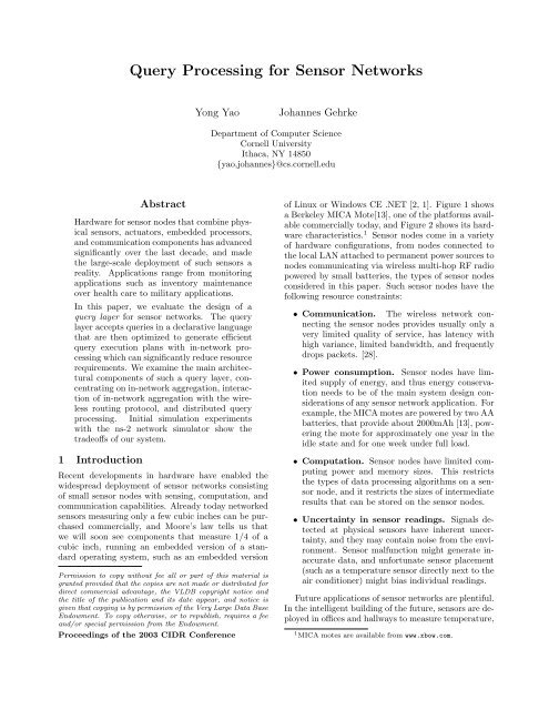
of Linux or Windows CE .NET [2, 1]. Figure 1 shows
a Berkeley MICA Mote[13], one of the platforms available
commercially today, and Figure 2 shows its hardware
characteristics. 1 Sensor nodes come in a variety
of hardware configurations, from nodes connected to
the local LAN attached to permanent power sources to
nodes communicating via wireless multi-hop RF radio
powered by small batteries, the types of sensor nodes
considered in this paper. Such sensor nodes have the
following resource constraints:
• Communication. The wireless network connecting
the sensor nodes provides usually only a
very limited quality of service, has latency with
high variance, limited bandwidth, and frequently
drops packets. [28].
• Power consumption. Sensor nodes have limited
supply of energy, and thus energy conservation
needs to be of the main system design considerations
of any sensor network application. For
example, the MICA motes are powered by two AA
batteries, that provide about 2000mAh [13], powering
the mote for approximately one year in the
idle state and for one week under full load.
• Computation. Sensor nodes have limited computing
power and memory sizes. This restricts
the types of data processing algorithms on a sensor
node, and it restricts the sizes of intermediate
results that can be stored on the sensor nodes.
• Uncertainty in sensor readings. Signals detected
at physical sensors have inherent uncertainty,
and they may contain noise from the environment.
Sensor malfunction might generate inaccurate
data, and unfortunate sensor placement
(such as a temperature sensor directly next to the
air conditioner) might bias individual readings.
Future applications of sensor networks are plentiful.
In the intelligent building of the future, sensors are deployed
in offices and hallways to measure temperature,
1 MICA motes are available from www.xbow.com.

Processor
Storage
Radio
Figure 1: A Berkeley MICA Mote
Communication
Range
Data Rate
Transmit Current
Receive Current
Sleep Current
4Mhz, 8bit MCU (ATMEL)
512KB
916Mhz Radio
(RF Monolithic)
100 ft
40 Kbits/sec
12 mA
1.8 mA
5 uA
Figure 2: Hardware Characteristics of a MICA Mote
noise, light, and interact with the building control system.
People can pose queries that are answered by
the sensor network, such as “Is Yong in his office”, or
“Is there an empty seat in the meeting room” Another
application is scientific research. As an example,
consider a biologist who may want to know of the existence
of a specific species of birds, and once such a
bird is detected, the bird’s trail should be mapped as
accurately as possible. In this case, the sensor network
is used for automatic object recognition and tracking.
More specific applications in different fields will arise,
and instead of deploying preprogrammed sensor networks
only for specific applications, future networks
will have sensor nodes with different physical sensors
for a wide variety of application scenarios and different
user groups. 2
In this paper, we develop a query layer for wireless
sensor networks. Our approach is motivated by the following
three design goals. First, we believe that declarative
queries are especially suitable for sensor network
interaction: Clients issue queries without knowing how
the results are generated, processed, and returned to
the client. Sophisticated catalog management, query
optimization, and query processing techniques will abstract
the user from the physical details of contacting
the relevant sensors, processing the sensor data,
and sending the results to the user. Thus one of the
main roles of the query layer is to process declarative
queries.
Our second design goal is motivated by the importance
of preserving limited resources, such as energy
2 The MICA motes already support temperature sensors,
light sensors, magnetometers, accelerometers, and microphones.
and bandwidth in battery-powered wireless sensor networks.
Data transmission back to a central node for
offline storage, querying, and data analysis is very expensive
for sensor networks of non-trivial size since
communication using the wireless medium consumes a
lot of energy. Since sensor nodes have the ability to
perform local computation, part of the computation
can be moved from the clients and pushed into the
sensor network, aggregating records, or eliminating irrelevant
records. Compared to traditional centralized
data extraction and analysis, In-network processing
can reduce energy consumption and reduce bandwidth
usage by replacing more expensive communication operations
with relatively cheaper computation operations,
extending the lifetime of the sensor network significantly.
For example, the ratio of energy spent in
sending one bit versus executing one instruction ranges
from 220 to 2900 in different architectures [29]. 3 Thus
the second main role of the query layer is to perform
in-network processing.
Different applications usually have different requirements,
from accuracy, energy consumption to delay.
For example, a sensor network deployed in a battlefield
or rescue region may only have a short life time
but a high degree of dynamics. On the other had, for a
long-term scientific research project that monitors an
environment, power-efficient execution of long-running
queries might be the main concern. More expensive
query processing techniques may shorten processing
time and improve result accuracy, but might use a lot
of power. The query layer can generate query plans
with different tradeoffs for different users.
In this paper, we propose and evaluate a database
layer for sensor networks; we call the component of
the system that is located on each sensor node the
query proxy. Architecturally, on the sensor node, the
query proxy lies between the network layer and the
application layer, and the query proxy provides higherlevel
services through queries.
Given the view of a sensor network as a huge distributed
database system, we would like to adapt existing
techniques from distributed and heterogeneous
database systems for a sensor network environment.
However, there are major differences between sensor
networks and traditional distributed and heterogeneous
database systems.
First, sensor networks have communication and
computation constraints that are very different from
regular desktop computers or dedicated equipment in
data centers, and query processing has to be aware of
these constraints. One way of thinking about such constraints
is the analogous interaction with the file systems
in traditional database systems [37]. Database
systems bypass the file system buffer to have direct
3 This is only a rule of thumb, since transmission range, bit
error rates, and instruction width influence this parameter significantly.

control over the disk. For a sensor network database
system, the analogous counterpart is the networking
layer, and for intelligent resource management we have
to ensure that the query processing layer is tightly integrated
with the networking layer. Second, the notion
of the cost of a query plan has changed, as the critical
resource in a sensor network is power, and query optimization
and query processing have to be adapted to
take this optimization criterion into account.
While developing techniques that address these issues,
we must not forget that scalability of our techniques
with the size of the network, the data volume,
and the query workload is an intrinsic consideration to
any design decision.
Overview of the paper. The remainder of the
paper is structured as follows. In the next section,
we introduce our model of a sensor network, sensor
data, and the class of queries that we consider in this
paper. We then demonstrate our algorithms to process
simple aggregate queries with in-network aggregation
(Section 3), and investigate the interaction between
the routing layer and the query layer (Section 4). We
discuss how to create query plans to evaluate more
complicated queries, and discuss query optimization
for specific types of queries (Section 5). In a thorough
simulation study, we examine the performance of our
approach, and compare and analyze the performance
of different query plans (Section 6).
2 Preliminaries
2.1 Sensor Networks
A sensor network consists of a large number of sensor
nodes [27]. Individual sensor nodes (or short, nodes)
are connected to other nodes in their vicinity through
a wireless network, and they use a multihop routing
protocol to communicate with nodes that are spatially
distant. Sensor nodes also have limited computation
and storage capabilities: a node has a general-purpose
CPU to perform computation and a small amount of
storage space to save program code and data.
We will distinguish a special type of node called a
gateway node. Gateway nodes are connected to components
outside of the sensor network through longrange
communication (such as cables or satellite links),
and all communication with users of the sensor network
goes through the gateway node. 4
Since sensors are usually not connected to a fixed
infrastructure, they use batteries as their main power
supply, and preservation of power is one of the main
design considerations of a sensor network [34]. This
makes reduction of message traffic between sensors
very important.
4 Relaxations of this requirement, such as communication
with the network via UAVs or via an arbitrary node are left
for future work.
SELECT {attributes, aggregates}
FROM {Sensordata S}
WHERE {predicate}
GROUP BY {attributes}
HAVING {predicate}
DURATION time interval
EVERY time span e
2.2 Sensor Data
Figure 3: Query Template
A sensor node has one or more sensors attached that
are connected to the physical world. Example sensors
are temperature sensors, light sensors, or PIR sensors
that can measure the occurrence of events (such as the
appearance of an object) in their vicinity. Thus each
sensor is a separate data source that generates records
with several fields such as the id and location of the
sensor that generated the reading, a time stamp, the
sensor type, and the value of the reading. Records
of the same sensor type from different nodes have the
same schema, and collectively form a distributed table.
The sensor network can thus be considered a large distributed
database system consisting of multiple tables
of different types of sensors.
Sensor data might contain noise, and it is often possible
to obtain more accurate results by fusing data
from several sensors [12]. Summaries or aggregates of
raw sensor data are thus more useful to sensor applications
than individual sensor readings [21, 10]. For
example, when monitoring the concentration of a dangerous
chemical in an area, one possible query is to
measure the average value of all sensor readings in that
region, and report whenever it is higher than some predefined
threshold.
2.3 Queries
We believe that declarative queries are the preferred
way of interacting with a sensor network. Rather
than deploying application-specific procedural code
expressed in a Turing-complete programming language,
we believe that sensor network applications are
naturally data-driven, and thus we can abstract the
functionality of a large class of applications into a common
interface of expressive queries. In this paper, we
consider queries of the simple form shown in Figure 3,
and we leave the design of a suitable query language
for sensor networks to future work. We also extend
the template to support nested queries, where the basic
query block shown in Figure 3 can appear within
the WHERE or HAVING clause of another query block.
Our query template has the obvious semantics: The
SELECT clause specifies attributes and aggregates
from sensor records, the FROM clause specifies the
distributed relation of sensor type, the WHERE clause
filters sensor records by a predicate, the GROUP BY

SELECT AVG(R.concentration)
FROM ChemicalSensor R
WHERE R.loc IN region
HAVING AVG(R.concentration) > T
DURATION (now,now+3600)
EVERY 10
Figure 4: Example Aggregate Query
clause classifies sensor records into different partitions
according to some attributes, and the HAVING clause
eliminates groups by a predicate. Note that it is possible
to have join queries by specifying several relations
in the FROM clause.
One difference between our query template and
SQL is that our query template has additional support
for long running, periodic queries. Since many sensor
applications are interested in monitoring an environment
over a longer time-period, long-running queries
that periodically produce answers about the state of
the network are especially important. The DURA-
TION clause specifies the life time of a query and the
EVERY clause determines the rate of query answers:
we compute a query answer every e seconds (see Figure
3 [21]). We call the process of computing a query
answer a round. The focus of this paper is the computation
of aggregate queries, in which a set of sensor
readings is summarized into a single statistic.
Note that our query template has only limited usage
for event-oriented applications. For example, to monitor
whether the average concentration of a chemical is
above a certain threshold, we can use the long-running
query shown in Figure 4, but there is a delay of 10
seconds between every recomputation of the average.
Event oriented applications are an interesting topic for
future research, as the query processing strategies that
we propose are optimized for long-running periodic
queries, and not event-oriented queries and triggers.
3 Simple Aggregate Query Processing
A simple aggregate query is an aggregate query without
Group By and Having clauses, a very popular class
of queries in sensor networks [21]. In this section we
outline how to process such simple aggregate queries.
Query processing strategies for more general queries
are discussed in Section 5.
3.1 In-Network Aggregation
A query plan for a simple aggregate query can be divided
into two components. Since queries require data
from spatially distributed sensors, we need to deliver
records from a set of distributed nodes to a central
destination node for aggregation by setting up suitable
communication structures for delivery of sensor
records within the network. We call this part of a
query plan its communication component, and we call
the destination node the leader of the aggregation. In
addition, the query plan has a computation component
that computes the aggregate at the leader and potentially
computes already partial aggregates at intermediate
nodes.
Recall that power is one of the main design desiderata
when devising query processing strategies for sensor
networks. If we coordinating both the computation
and communication component of a query plan, we
can compute partial aggregates at intermediate nodes
as long as they are well-synchronized; this reduces the
number of messages sent and thus saves power. We
address synchronization in the next section, and consider
here three different techniques on how to integrate
computation with communication:
Direct delivery. This is the simplest scheme.
Each source sensor node sends a data packet consisting
of a record towards the leader, and the multi-hop
ad-hoc routing protocol will deliver the packet to the
leader. Computation will only happen at the leader
after all the records have been received.
Packet merging. In wireless communication, it is
much more expensive to send multiple smaller packets
instead of one larger packet, considering the cost of reserving
the channel and the payload of packet headers.
Since the size of a sensor record is usually small and
many sensor nodes in a small region may send packets
simultaneously to process the answer for a round
of a query, we can merge several records into a larger
packet, and only pay the packet overhead once per
group of records. For exact query answers with holistic
aggregate operators like Median, packet merging is
the only way to reduce the number of bytes transmitted
[10].
Partial aggregation. For distributive and algebraic
aggregate operators [10], we can incrementally
maintain the aggregate in constant space, and thus
push partial computation of the aggregate from the
leader node to intermediate nodes. Each intermediate
sensor node will compute partial results that contain
sufficient statistics to compute the final result.
3.2 Synchronization
To perform packet merging or partial aggregation, we
need to coordinate sensor nodes within the communication
component of a query plan. A node n needs
to decide whether other nodes n 1 , . . . , n k are going to
route data packets through n; in this case n has the
opportunity of either packet merging or partial aggregation.
Thus a node n needs to build a list of nodes
it is expecting messages from, and it needs to decide
how long to wait before sending a message to the next
hop.
For duplicate sensitive aggregate operators, like
SUM and AVG, one prerequisite to perform partial aggregation
is to send each record only once, otherwise
duplicate records might appear in partially aggregated

esults and bias the result, thus a simple spanning
tree might be a suitable communication structure. For
other aggregate operators, including MAX and MIN,
it is possible to send multiple copies of a record along
different paths without any influence on the query accuracy;
thus a suitable communication structure might
be a DAG rooted at the leader.
The task of synchronization in this tree or DAG is
then for each node in each round of the query to determine
how many sensor readings to wait for and when
to perform packet merging or partial aggregation.
Incremental Time Slot Algorithm. Let us first
discuss the following simple algorithm. At the beginning
of a round, each sensor node sets up a timer,
and waits for a special waiting time for data packets
from its children in the spanning tree or DAG to arrive.
The length of the timer at node n is set to the
depth of the structure rooted at n times a standardized
time slot. However, this algorithm has a large
cost in reality. First, it is very difficult to determine in
advance how long a node needs to collect records from
its children. The time to process the data, schedule
the packet, reserve the channel, and retransmit packets
due to frequently temporary link failures can vary
significantly. Although the expected size of a time slot
is small, it has a heavy tail with a big variance. But
if the time slot is too large, the accumulated delay at
the leader could be very long if the depth of the tree
or DAG is large.
Second, with frequent link failures, it is expensive to
update the time-out value every time the structure of
the communication structure changes. Although most
broken links can be repaired locally, repairs may effect
the depth of a large number of nodes, and it is expensive
to update the timer for all of these nodes. Third,
sensor nodes are never completely time-synchronized
unless expensive time synchronization protocols or frequent
GPS readings are used.
Our Approach. We take a very pragmatic approach
to synchronization. Note that for a longrunning
query, the communication behavior between
two sensors n and p is consistent over short periods of
time, so it is possible to use historical information to
predict future behavior. Assuming that p is the parent
of node n. After p receives a record from n, it may
expect to receive another record from n in the next
round, and thus p adds n to its waiting list. However,
such prediction may fail in two cases. First, the
parent of node n may change in the next round if n
reroutes and has a new parent due to network topology
changes and route updates. Second, n could perform
a local selection on its records, and only send a record
to p if the selection condition is satisfied. Such conditions
are only satisfied from time to time, and make
the prediction at p fail.
In our approach, we use a timer to recover from false
prediction at parent nodes. On the other hand, since
a child node is able to determine whether its parent
is expecting a packet from it, the child can generate a
notification packet if its parent’s prediction is wrong.
We found that this bi-directional prediction approach
model the relationship between the parent and child
nodes very well in practice, as shown in Section 6.
4 Routing and Crash Recovery
To execute simple aggregate queries, sensor nodes have
to send their records to a leader, aggregate them into a
final result, and then deliver the final result to the gateway
node. Note that a sensor node can only communicate
directly with other nodes in its vicinity, limited by
the transmission power of the wireless radio. To send
messages to a distant node, a multi-hop route connecting
the node to the destination has to be established
in advance. A packet is forwarded by internal nodes
along the route until the packet reaches its destination.
Note that this structure is similar in both wired
and wireless networks, but there are major differences.
In a wired network, the network structure is almost
fixed and most routing problems are handled at a few
backbone routers. In a wireless network, such as a
sensor network, limited connectivity requires all nodes
to participate in routing. In addition, the low quality
of the communication channel and frequent topology
changes make the network quite unstable. Thus more
complicated routing protocols are required for wireless
networks.
The networking community has developed many
different ad-hoc network routing algorithms. A separate
routing layer in the protocol stack provides a send
and receive interface to the upper layer and hides the
internals of the wireless routing protocol. In this section,
we show that a routing layer for a query processing
workload has slightly different requirements than
a traditional ad-hoc routing layer, and then we outline
some initial thoughts on how to adapt AODV [26], a
popular wireless routing protocol, to a query processing
workload.
4.1 Wireless Routing Protocols
The two main tasks of a routing protocol are route discovery
and route maintenance. Route discovery establishes
a route connecting a pair of nodes when required
by the upper layer, and route maintenance repairs the
route in case of link failures. Many wireless routing
protocols have been proposed and implemented,
mostly aimed at ad-hoc networks. A distributed and
adaptive routing protocol, in which nodes share the
routing decision and nodes can change routes according
to the network status, is more suitable to sensor
networks. Such protocols can be further classified
into proactive, reactive and hybrid routing protocols.
Proactive routing protocols, like DSDV [25], may set
up routes between any pair of nodes in advance; while
reactive routing protocols create and repair routes only

on demand. Hybrid routing protocols, e.g. ZRP [11],
combine both properties of proactive and reactive protocols.
AODV is a typical reactive routing algorithm. It
builds routes between nodes only as desired by the application
layer. There are several reasons why we use
AODV as the routing protocol for our study. First,
reactive routing protocols scale to large-size networks,
such as sensor network with thousands of nodes. Second,
AODV does not generate duplicate data packets,
which is a requirement to do in-network aggregation
for duplicate-sensitive aggregate operators. Finally,
AODV is a popular ad-hoc network routing protocol
and it is implemented in several simulators. Although
our discussion is based on AODV, our observations
apply to other routing protocols as well.
4.2 Extensions to the Network Interface
Recall from Section 3 that we can optimize aggregate
operators through in-network aggregation, such
as packet merging and partial aggregation at internal
nodes. These techniques require internal nodes to
intercept data packets passing through them to perform
packet merging or partial aggregation. However,
with the traditional “send and receive” interfaces of
the network layer, only the leader will receive the data
packets. The network layer on an internal node will
automatically forward the packages to the next hop towards
the destination, and the upper layer is not aware
of data packets traveling through the node. This functionality
is sufficient for direct delivery of packets to
a destination node, but to implement in-network aggregation,
a node needs the capability to “intercept”
packages that are not destined for itself; the query
layer needs a way to communicate to the network layer
which and when it wants to intercept packages that are
destined for the leader [14].
With filters [14], the network layer will first pass
a package through a set of registered functions that
can modify (and possibly even delete) the packet. In
case of the query layer, if a node n is scheduled to
aggregate data from all children nodes, it can intercept
all data packets received from the children nodes
and cache the aggregated result. At a specific time,
n will generate a new data packet and send it to the
leader. All this happens completely transparently to
the network layer.
4.3 Modifications to Wireless Routing Protocols
Existing wireless routing protocols are not designed
for the communication patterns exhibited by a query
processing layer: they are designed for point-to-point
communication, and are usually evaluated by selecting
two random nodes and establishing and maintaining
a communication path between them. A sensor
network with a query layer has a significantly different
communication pattern: Many source nodes send
tuples to a common node, like a leader of an aggregation,
or a gateway node. In addition, in a regular
ad-hoc network, a node has no knowledge about the
communication intents of neighboring nodes, whereas
in a sensor network, data transfer to the leader node is
usually synchronized to perform aggregation. Thus a
node can often estimate when neighboring nodes (such
as children in a spanning tree) will send messages to
it. We describe here a series of enhancements to one
specific routing protocol, AODV [26], although we believe
that our techniques are general enough to apply
to any wireless routing protocol.
Route initialization. Before sending data packets
to the leader, each sensor has to establish a route
to the leader, or determine who is the next hop in
the DAG or spanning tree. Instead of initializing the
route for each node separately from the source node
as it would happen in AODV, we can create all the
routes together by broadcasting a route initialization
message originating at the leader of the aggregation.
The message contains a hop count which is used for
nodes to determine their depth in the tree. Using this
initial broadcast, nodes can save the reverse path as
the route to the leader.
Route maintenance. Reliability plays a very important
role in in-network aggregation. Since each
data packet contains an aggregate result from multiple
sensor nodes, dropping a data packet, especially
if near the leader, will seriously decrease the accuracy
of the final result. The problem is more serious in sensor
networks, in which link or node failures happens
frequently. We describe two techniques that improve
AODV in case of failures.
Local Repair. In AODV, when a broken link is detected,
the source node n broadcasts a request to find
an alternative route. An internal node n ′ cannot reply
to the request unless n ′ has a “fresher route” to the
leader than n. The efficiency of the local repair algorithm
depends on how fast a node can find an up-todate
route in its neighborhood, and AODV uses a sequence
number to reflect route “freshness”. Given that
query processing has a very regular communication
structure, in which many of nodes want to route packets
to the same destination, we can extend AODV’s
idea of a sequence number to repair broken routes more
efficiently. Since a broken link has no effect on other
nodes which are close to the leader, we integrate the
depth of a node into the packet sequence number to
differentiate sequence numbers between nodes that are
spatially close. The new algorithm does not depend
on the exact depth of a node to compute the new sequence
number; a rough approximation that preserves
relative depths is sufficient. Using an approximation
to depth prevents a node from updating the depths of
all nodes on the path to the leader after the broken

oute is repaired, which is a very expensive operation.
Bunch Repair. Local repair can find a new route to
bypass a broken link or node in the neighborhood, but
it may fail if significant topology changes happen, or a
large number of links fail simultaneously due to a spatial
disturbance (e.g., large noise in an area). In this
case, it is cheaper to repair all routes directly from the
leader (by re-broadcasting the route initialization message).
Some feedback is required at the leader to active
this operation to avoid unnecessary re-initialization.
In this first version of our query layer, we re-broadcast
a the tree initialization message whenever we receive
less than a user-defined fraction of all tuples within an
user-defined time interval. (We can calculate the number
of tuples that contributed to an aggregate query
by adding a COUNT attribute to the partial state of
all aggregates.)
5 Query Plans
In this section, we outline the structure of a query
plan and discuss general techniques to process sensor
network queries.
5.1 Query Plan Structure
Let us consider an example query that we will use to illustrate
the components of a query plan. Consider the
query “What is the quietest open classroom in Upson
Hall”. 5 Assume that the computation plan for this
query is to first compute the average acoustic value of
each open classroom and then to select the room with
the smallest number. There are two levels of aggregation
in this plan: (1) to compute the average value
of each qualified classroom, and (2) to select the minimum
average over all classrooms. The output of the
first level aggregation is the input to the second level
aggregation.
Users may pose even more complicated queries with
more levels of aggregations, and more complex interactions.
A query plan decides how much computation
is pushed into the network and it specifies the role and
responsibility of each sensor node, how to execute the
query, and how to coordinate the relevant sensors. A
query plan is constructed by flow blocks, where each
flow block consists of a coordinated collection of data
from a set of sensors at the leader node of the flow
block. The task of a flow block is to collect data from
the relevant sensor nodes and to perform some computation
at the destination or internal nodes. A flow
block is specified by different parameters such as the
set of source sensor nodes, a leader selection policy,
the routing structure used to connect the nodes to the
leader (such as a DAG or tree), and the computation
that the block should perform.
5 Upson Hall is a building with several classrooms located on
the Cornell Campus.
A query plan consists of several flow blocks. Creating
a flow block and its associated communication and
computation structure (which we also call a cluster)
uses resources in the sensor network. We need to expend
messages to maintain the cluster through a periodical
heart beat message in which the leader indicates
that it is still alive; in case the cluster leader fails, a
costly leader election process is required. In addition,
a cluster might also induce some delay, as it coordinates
computation among the sensors in the cluster.
Thus if we need to aggregate sensor data in a region,
we should reuse existing clusters instead of creating a
new cluster, especially if the data sources are loosely
distributed over a larger area, in which case the maintenance
cost increases. On the other hand, we should
create a flow block if it significantly reduces the data
size at the leader node and saves costly transmission
of many individual records.
It is the optimizer’s responsibility to determine the
exact number of flow blocks and the interaction between
them. Compared to a traditional optimizer, we
would like to emphasize two main differences. First,
the optimizer should try to reduce communication
cost, while satisfying various user constraints such as
accuracy of the query, or a user-imposed maximum
delay of receiving the query answers. The second difference
lies in the building blocks of the optimizer.
Whereas in traditional database systems a building
block is an operator in the physical algebra, our basic
building block in a sensor database system is a flow
block, which specifies both computation and communication
within the block.
5.2 Query Optimization
In this section we will discuss how to create a good
query plan for more complicated queries. Our discussion
stays at the informal level with the goal to help
us decide what meta-data we need for the optimizer in
the systems catalog. We would like to emphasize that
creation of the best query plan for an arbitrary query is
a hard problem, and our work should be considered as
an initial step towards the design and implementation
of a full-fledged query optimizer. We leave experimental
evaluations of different query plans to section 6,
and the design and implementation of a full-fledged
optimizer to future work.
Extension to GROUP BY and HAVING
Clauses. Let us consider an aggregate query with
GROUP BY and HAVING clauses. The following query
computes the average value for each group of sensors
and filters out groups with average smaller than some
threshold.
(Q1) SELECT
FROM
GROUP BY
HAVING
D.gid, AVG(D.value)
SensorData D
D.gid
AVG(D.value)>Threshold

There are two alternative plans for this query. We
can create a flow block for each group, or we can create
a flow block that is shared by multiple groups.
To create a separate flow block can aggregate sensor
records of the same group as soon as possible,
shorten the path length, and allow to apply the predicate
of the HAVING clause to the aggregate results earlier,
which saves more communication if the selectivity
of the predicate is low. The optimizer should take several
parameters into account to make the best plan.
One parameter is the overlap of the distribution of the
physical locations of the sensors that belong to the different
groups. If sensors that below to a single group
are physically close, it is better to create a separate
flow block to aggregate them together, since the communication
cost to aggregate close-by sensors is usually
low. However, if sensors from different groups are
spatially interspersed, it is more efficient to construct
a single flow block shared by all groups.
Joins. The computation part of a flow block does
not need to be an aggregate operator. It is possible to
add join operators to our query template and define
flow blocks with joins. Joins will be common in applications
for tracking or object detection. For example,
a user may pose a query to select all objects detected
in both regions R1 and R2. The following query has a
join operator to connect sensor detections in the two
regions.
(Q2) SELECT
FROM
WHERE
oid
SensorData D1, SensorData D2
D1.loc IN R1 AND D2.loc IN R2
AND D1.oid = D2.oid
Join operators represent a wide range of possible
data reductions. Depending on the selectivity of the
join, it is possible to either reduce or increase the resulting
data size. If the join increases the result size,
it is more expensive to compute the join result at the
leader instead of having the leader send out the tuples
from the base relation. Relevant catalog data to
make an informed decision concerns the selectivity of
the join and the location of the leader.
6 Experimental Evaluation
6.1 Experimental Setup
We have started to implement a prototype of our query
processing layer in the ns-2 network simulator [4]. Ns-2
is a discrete event simulator targeted at simulating network
protocols to highest fidelity. Due to the strong interaction
between the network layer and our proposed
query layer, we decided to simulate the network layer
to a high degree of precision, including collisions at
the MAC layer, and detailed energy models developed
by the networking community. In our experiments, we
used IEEE 802.11 as the MAC layer [36], setting the
communication range of each sensor to 50m and assuming
bi-directional links; this is the setup used in
most other papers on wireless routing protocols and
sensor networks in the networking community [14].
In our energy model the receive power dissipation is
395mW, and the transmit power dissipation is 660mW
[14]. (This matches numbers from previous studies.)
There are many existing power-saving protocols that
can turn the radio to idle [35, 27], thus we do not take
the energy consumption in the idle state into account.
Sensor readings were modeled as 30 bytes tuples. 6
6.2 Simple Aggregate Query
Let us first investigate experimentally the effects of innetwork
aggregation. We run a simple aggregate query
that computes the average sensor value over all sensor
nodes every 10 seconds for 10 continuous rounds. Sensors
are randomly distributed in a query region with
different size. The gateway node, which is located in
the left-upper corner of the query region, is the leader
of the aggregate query. Each experiment is the average
of ten runs with randomly generated maps.
We first investigate the effect of in-network aggregation
on the average dissipated energy per node assuming
a fixed density of sensor nodes throughout the
network (in this experiment we set the average sensor
node density to 8 sensors in a region of 100m × 100m).
Figure 5 shows the effect of increasing the number
of sensors on the average energy usage of each sensor.
In the best case, every sensor only needs to send one
merged data packet to the next hop in each round,
no matter how many sensors are in the network. The
packet merge curve increases slightly as intermediate
packets get larger as the number of nodes grows. Without
in-network aggregation, a node n has to send a
data packet for each node whose route goes through
n, so energy consumption increases very fast.
We also investigated the effect of in-network aggregation
on the delay of receiving the answer at the gateway
node as shown in Figure 6. When the network size
is very small, in-network aggregation introduces little
extra delay due to synchronization, however as the network
size increases, direct delivery induces much larger
delay due to frequent conflicts of packets at the MAC
layer.
6.3 Routing
To test the efficiency of our improved local repair algorithm,
we ran a simple aggregate query which computes
the average over all sensor readings every 10 seconds.
In this experiment, 200 sensors are randomly
distributed in a 500m*500m area. (For other experiments
the numbers were qualitatively similar.) We
6 See the discussion of future work in Section 8 for drawbacks
of our current experimental setup.

!"#
$%
$&
%
! "#
!
Average Dissipated Energy Per Node (J)
0.05
AODV
0.045
AODV with Improved
Local Repair
0.04
0.035
0.03
0.025
0.02
0.015
0.01
0.005
0
0% 5% 10% 15% 20% 25%
Link Failure Ratio
Average Dissipated Energy Per Node (J)
0.01
0.009
0.008
0.007
0.006
0.005
0.004
0.003
0.002
0.001
0
AODV with Improved
Local Repair
Bunch Repair
(Threshold=80%)
0% 5% 10% 15% 20% 25%
Link Failure Ratio
Figure 5: Average Dissipated
Energy
vs. Network
Figure 6: Average Delay
Size
Figure 7: Improved Local
Repair Algorithm
Figure 8: Effect of Bunch
Repair
Accuracy
1
0.9
0.8
0.7
0.6
0.5
0.4
0.3
0.2
AODV with
Improved Local
Repair
Bunch Repair
(Threshold=80%)
Average Sensor Dissipated Energy Per Round
0.0006
0.0005
0.0004
0.0003
0.0002
0.0001
Plan 1
Plan 2
0.1
0
0% 5% 10% 15% 20%
Link Failure Ratio
0
10% 50% 100%
Selectivity
Figure 9: Cornell Map Used in Exp.
Figure 10: Result Accuracy
Figure 11: Aggregate Query
introduced random link failures quantified as the percentage
of crashed links in a round, and we tested their
influence on the routing protocols. Figure 7 shows the
comparison between AODV and AODV with our improved
local repair algorithm using different link failure
rates. As the link failure rate increases, AODV
uses much more energy than the algorithm with improved
local repair.
We evaluated bunch repair experimentally using the
Cornell campus as the query region. About 150 sensors
are virtually distributed close to buildings or along
main streets; see Figure 9. Figure 8 compares the improved
version of AODV with and without bunch repair.
The threshold to active route reinitialization is
to 80 percent of the tuples. The two algorithms are
very close when link failure ratio is low, but our new
algorithm saves much energy after the failure ratio becomes
larger. This is because bunch repair generates
much fewer route request and reply messages, especially
when more links fail simultaneously.
Figure 10 shows the influence of bunch repair on the
final result accuracy. 7 If several local repairs fail a serious
topology change happens, and thus many nodes
are disconnected temporarily. A bunch repair will be
automatically activated in this case, and thus the accuracy
of AODV with bunch repair does not decrease
compared to AODV while at the same time the average
dissipated energy per node will be much lower
compared to AODV.
6.4 Query Plans
We first investigate the benefit of creating a flow block
according to the data reduction rate at the leader using
the following query:
(Q3) SELECT AVG(value)
FROM Sensor D
WHERE D.loc IN [(400,400),(500,500)]
HAVING AVG(value)>t
7 The accuracy is measured at the end of each round. Packets
are dropped at internal nodes if they belong to the previous
round.

Let us consider two different query plans for Query
Q3. In Plan 1, we use an existing flow block which
covers the whole network. This flow block is also used
to collect system catalog information, thus it does not
incur additional maintenance cost. In Plan 2, we construct
a new flow block for Query Q3 just inside the
query region, where we first compute the average at a
leader of this block, and then send qualifying averages
to the gateway node.
Both plans may perform the HAVING operation as a
filter over the average value of the sensor reading, at
the gateway for Plan 1, but the leader node in Plan 2.
The result in Figure 11 shows that if the selectivity of
the HAVING operator is close to 100% and thus the computation
at the leader does not reduce the number of
outgoing averages, then there is not much difference in
terms of the average dissipated sensor energy for each
round of the query. Plan 2 spends only a little more
energy on maintenance of the additional flow block.
However, as the leader discards aggregated data packets
with higher and higher probability, Plan 2 is a much
better choice. It reduces the traffic flow significantly
through aggregation at the leader much closer to data
sources, compared to the gateway node of Plan 1.
Next, we evaluate different query plans for Query
Q1, a query with a GROUP BY clause. Assume that
there are four different groups. Let us consider three
simple cases: In the distributed case, sensors that below
to a single group are physically close, but far away
from other groups. In the close-by case, the groups are
close to each other, but they do not overlap, whereas
in the overlap scenario, all four groups are in the same
area. We again consider two different query plans for
this query. Plan 1 creates one big cluster to be shared
by all groups. Aggregation within each group happens
at the global cluster leader. Plan 2 creates a separate
cluster for each group, and aggregates only the tuples
relevant for each group at the respective cluster leader.
Figure 16 shows the different spatial distributions of
the four groups for the three cases.
We can see from Figure 12 that if the groups are
physically close, then there is no big difference between
Plans 1 and 2. However, creating one big cluster
increases the connectivity of the cluster, and reduces
the risk of network partitioning within a cluster. If
the four groups are spatially distant from each other,
Plan 2 is more efficient as the selection at the aggregation
leaders can reduce the number of data packets
for transmission back to the gateway node. In the last
scenario, where the different groups of sensors are randomly
distributed, Plan 1 outperforms Plan 2, since
the cost to collect data records at the leader is high.
Figures 13 and 14 show the influence of operator
selectivity on the two plans in the previous experiment
for two different sensor topologies, the distributed
topology in Figure 13 and the overlap topology
in Figure 14. The experiment shows that operator
selectivity has a strong influence on plan performance,
although the sensor topology has a much larger impact.
Next we consider the Join Query Q2. Again we
consider two query plans to evaluate this query. In
Plan 1, sensors send all tuples back to the gateway
without any in-network computation; Plan 2 creates
a flow block for the Join operator inside the query
region. In Plan 2, in case the join reduces the data
size at the leader, the leader sends the result of the
join back to the gateway, otherwise, the leader sends
all individual data records to the gateway for the join
to be performed there.
Figure 15 shows that the cost to collect data at the
leader is non-trivial. If the join operator at the leader
fails to reduce the data size, then the total energy consumption
at the node increases. Thus the optimizer
needs to estimate the selectivity of the join operator,
and it needs statistics in the systems catalog to make
the right decision.
7 Related Work
Research of routing in ad-hoc wireless networks has
a long history [17, 30], and a plethora of papers has
been published on routing protocols for ad-hoc mobile
wireless networks [25, 16, 5, 26, 24, 8, 15]. All these
routing protocols are general routing protocols and do
not take specific application workloads into account,
although we believe that most of these protocols can
be augmented with the techniques similar to those that
we propose in Section 4. The SCADDS project at USC
and ISI explores scalable coordination architectures for
sensor networks [9], and their data-centric routing algorithm
called directed diffusion [14] first introduced
the notion of filters that we advocate in Section 4.2.
There has been a lot of work on query processing
in distributed database systems [40, 7, 23, 39, 18], but
as discussed in Section 1, there are major differences
between sensor networks and traditional distributed
database systems. Most related is work on distributed
aggregation, but existing approaches do not consider
the physical limitations of sensor networks [33, 38].
Aggregate operators are classified by their properties
by Gray et al. [10], and an extended classification with
properties relevant to sensor network aggregation has
been proposed by Madden et al. [21].
The TinyDB Project at Berkeley also investigates
query processing techniques for sensor networks including
an implementation of the system on the Berkeley
motes and aggregation queries [19, 20, 21, 22].
Other relevant areas include work on sequence
query processing [31, 32], and temporal and spatial
databases [41].

!
Figure 12: Impact of Sensor
Distributions to Different
Query Plan
Average Sensor Dissipated Energy Per Round
0.0016
0.0014
0.0012
0.001
0.0008
0.0006
0.0004
0.0002
0
Plan 1
Plan 2
0% 20% 40% 60% 80% 100%
Selectivity
Figure 13: Distributed
Topology
Average Sensor Dissipated Energy Per Round
0.0016
0.0014
0.0012
0.0010
0.0008
0.0006
0.0004
0.0002
0.0000
0% 20% 40% 60% 80% 100%
Selectivity
Plan 1
Plan 2
Figure 14: Overlap Topology
Average Sensor Dissipated Energy Per Round
0.01
0.009
0.008
0.007
0.006
0.005
0.004
0.003
0.002
0.001
0
Plan 1
Plan 2
0% 50% 100% 150%
Join Selectivity
Figure 15: Join Query
Physical distribution:
Location of the four sensor groups
distributed [100,100,200,200] [100,400,200,500] [400,100,500,200] [400,400, 500,500]
close-by [100,100,200,200] [100,200,200,300] [200,100,300,200] [200,200,300,300]
overlap Sensors of all groups are randomly distributed [100,100,300,300]
Figure 16: Query Characteristics
8 Conclusions
Sensor networks will become ubiquitous, and the
database community has the right expertise to address
the challenging problems of tasking the network and
managing the data in the network. We described a
vision of processing queries over sensor networks, and
we discussed some initial steps in in-network aggregation,
implications on the routing layer, and query
optimization. We have started at Cornell to design
and implement a prototype that allows us to experiment
with the design space of various algorithms and
data structures [6].
Future work. This work opens a plethora of new
research directions at the boundary of database systems
and networking. First, we believe that TDMA
MAC protocols will be very important in powerconstrained
sensor networks [27], and we plan to investigate
the interaction of a TDMA MAC layer with
routing and query processing in future work. In addition,
our current simulation assumes bidirectional
links, which is usually not true in practice. Having
filters as an additional interface to the routing layer
leaves many open questions, such as an efficient implementation
of filters, the order in which filters should
be evaluated, handling of conflicting actions, etc. We
assumed very simple SQL blocks as query templates
without discussing a full-fledges spatio-temporal query
language whose design is a challenging topic for future
work. In addition, we only scratched the surface of
query processing, metadata management, and query
optimization, and much work needs to be done multiquery
optimization, distributed triggers, and the design
of benchmarks. We anticipate that the emergence
of new applications, as well as the implementation and
usage of our prototype system will lead to other research
directions. We believe that sensor networks will
be a fruitful research area for the database community
for years to come.
Acknowledgments. We thank the DARPA SensIT
community for helpful discussions. Praveen Sheshadri
and Philippe Bonnet made influential initial
contributions to Cougar. The Cornell Cougar Project
is supported by DARPA under contract F-30602-99-
0528, NSF CAREER grant 0133481, the Cornell Information
Assurance Institute, Lockheed Martin, and by
gifts from Intel and Microsoft. Any opinions, findings,
conclusions or recommendations expressed in this material
are those of the authors and do not necessarily
reflect the views of the sponsors.
References
[1] www.microsoft.com/windows/embedded/ce.net.
[2] www.redhat.com/embedded.
[3] ACM SIGMOBILE. Proceedings of MOBICOM 1998.
ACM Press.
[4] L. Breslau, D. Estrin, K. Fall, S. Floyd, J. Heidemann,
A. Helmy, P. Huang, S. McCanne, K. Varadhan,
Y. Xu, and H. Yu. Advances in network simulation.
IEEE Computer, 33(5):59–67, May 2000.

[5] J. Broch, D. A. Maltz, D. B. Johnson, Y.-C. Hu, and
J. Jetcheva. A performance comparison of multi-hop
wireless ad hoc network routing protocols. [3], pages
85–97.
[6] M. Calimlim, W. F. Fung, J. Gehrke, D. Sun,
and Y. Yao. Cougar Project web page.
www.cs.cornell.edu/database/cougar.
[7] S. Ceri and G. Pelagatti. Distributed Database Design:
Principles and Systems. MacGraw-Hill (New
York NY), 1984.
[8] S. Das, C. Perkins, and E. Royer. Performance comparison
of two on-demand routing protocols for ad hoc
networks. In INFOCOM 2000, pages 3–12. IEEE.
[9] D. Estrin, R. Govindan, J. Heidemann, and S. Kumar.
Next century challenges: Scalable coordination
in sensor networks. In MOBICOM 1999, pages 263–
270. ACM Press.
[10] J. Gray, S. Chaudhuri, A. Bosworth, A. Layman,
D. Reichart, M. Venkatrao, F. Pellow, and H. Pirahesh.
Data cube: A relational aggregation operator
generalizing group-by, cross-tab, and sub-totals. Data
Mining and Knowledge Discovery, 1(1):29–53, 1997.
[11] Z. Haas. The zone routing protocol (ZRP) for wireless
networks. IETF MANET, Internet Draft, 1997.
[12] D. L. Hall and J. Llinas, editors. Handbook of Multisensor
Data Fusion. CRC Press, 2001.
[13] J. Hill and D. Culler. A wireless embedded sensor
architecture for system-level optimization. Submitted
for publication, 2002.
[14] C. Intanagonwiwat, R. Govindan, and D. Estrin. Directed
diffusion: A scalable and robust communication
paradigm for sensor networks. In MOBICOM
2000, pages 56–67. ACM Press.
[15] P. Johansson, T. Larsson, N. Hedman, B. Mielczarek,
and M. Degermark. Scenario-based performance analysis
of routing protocols for mobile ad-hoc networks.
In MOBICOM 1999, pages 195–206. ACM Press.
[16] D. B. Johnson and D. A. Maltz. Dynamic source routing
in ad hoc wireless networks. In Mobile Computing.
Kluwer Academic Publishers, 1996.
[17] J. Jubin and J. D. Tornow. The DARPA packet radio
network protocol. Proceedings of the IEEE, 75(1):21–
32, Jan. 1987.
[18] D. Kossmann. The state of the art in distributed query
processing. Computing Surveys, 32, 2000.
[19] S. Madden and M. J. Franklin. Fjording the stream:
An architecture for queries over streaming sensor data.
In ICDE 2002.
[20] S. Madden and J. M. Hellerstein. Distributing queries
over low-power wireless sensor networks. In SIGMOD
2002.
[21] S. R. Madden, M. J. Franklin, J. M. Hellerstein, and
W. Hong. Tag: A tiny aggregation service for ad-hoc
sensor networks. In OSDI 2002.
[22] S. R. Madden, R. Szewczyk, M. J. Franklin, and
D. Culler. Supporting aggregate queries over ad-hoc
sensor networks. In Workshop on Mobile Computing
and Systems Applications (WMCSA), 2002.
[23] M. T. Özsy and P. Valduriez. Principles of Distributed
Database Systems. Prentice Hall, Englewood Cliffs,
1991.
[24] V. D. Park and M. S. Corson. A highly adaptive
distributed routing algorithm for mobile wireless networks.
In INFOCOM 1997. IEEE.
[25] C. Perkins and P. Bhagwat. Highly dynamic
destination-sequenced distance-vector routing
(DSDV) for mobile computers. In SIGCOMM
1994 , pages 234–244. ACM Press.
[26] C. E. Perkins. Ad hoc on demand distance
vector (aodv) routing. Internet Draft,
http://www.ietf.org/internet-drafts/draft-ietf-manetaodv-04.txt,
October 1999.
[27] G. J. Pottie and W. J. Kaiser. Embedding the Internet:
wireless integrated network sensors. Communications
of the ACM, 43(5):51–51, May 2000.
[28] G. J. Pottie and W. J. Kaiser. Wireless integrated network
sensors. Communications of the ACM, 43(5):51–
58, 2000.
[29] V. Raghunathan, C. Schurgers, S. Park, and M. B. Srivastava.
Energy-aware wireless microsensor networks.
IEEE Signal Processing Magazine, 19(2):40–50, 2002.
[30] N. Schacham and J. Westcott. Future directions in
packet radio architectures and protocols. Proceedings
of the IEEE, 75(1):83–99, January 1987.
[31] P. Seshadri, M. Livny, and R. Ramakrishnan. Seq: A
model for sequence databases. In ICDE 1995. IEEE
Computer Society.
[32] P. Seshadri, M. Livny, and R. Ramakrishnan. The design
and implementation of a sequence database system.
In VLDB 1996, pages 99–110. Morgan Kaufmann.
[33] A. Shatdal and J. F. Naughton. Adaptive parallel
aggregation algorithms. In SIGMOD 1995, pages 104–
114.
[34] T. Simunic, H. Vikalo, P. Glynn, and G. D. Micheli.
Energy efficient design of portable wireless systems.
In ISLPED 2000, pages 49–54. ACM Press.
[35] S. Singh, M. Woo, and C. S. Raghavendra. Poweraware
routing in mobile ad hoc networks. [3], pages
181–190.
[36] I. C. Society. Wireless LAN medium access control
(mac) and physical layer specification. IEEE Std
802.11, 1999.
[37] M. Stonebraker. Operating system support for
database management. CACM, 24(7):412–418, 1981.
[38] W. P. Yan and P.-Å. Larson. Eager aggregation and
lazy aggregation. In VLDB 1995. Morgan Kaufmann.
[39] C. Yu and W. Meng. Principles of Database Query
Processing for Advanced Applications. Morgan Kaufmann,
San Francisco, 1998.
[40] C. T. Yu and C. C. Chang. Distributed query processing.
ACM Computing Surveys, 16(4):399–433, Dec.
1984.
[41] C. Zaniolo, C. S., C. Faloutsos, R. Snodgrass, V. S.
Subrahmanian, and R. Zicari, editors. Advanced
Database Systems. Morgan Kaufmann, San Francisco,
1997.