- Page 1:
AIMMS Optimization Modeling AIMMS 3
- Page 4 and 5:
Copyright c○ 1993-2006 by Paragon
- Page 6 and 7:
vi About Aimms Stand-alone applicat
- Page 8 and 9:
viii Contents 3 Algebraic Represent
- Page 10 and 11:
x Contents Part IV Intermediate Opt
- Page 12 and 13:
xii Contents 22 A Facility Location
- Page 14 and 15:
xiv Preface Part IV—Data Managem
- Page 16 and 17:
xvi Preface What’s in the Optimiz
- Page 18 and 19:
xviii Preface tleneck capacity iden
- Page 20 and 21: xx Preface
- Page 23 and 24: Chapter 1 Background This chapter g
- Page 25 and 26: 1.3. The role of mathematics 5 Mode
- Page 27 and 28: 1.4. The modeling process 7 1.4 The
- Page 29 and 30: 1.5. Application areas 9 Planning m
- Page 31 and 32: 1.5. Application areas 11 The resul
- Page 33 and 34: 1.6. Summary 13 A different situati
- Page 35 and 36: 2.1. Formulating linear programming
- Page 37 and 38: 2.1. Formulating linear programming
- Page 39 and 40: 2.1. Formulating linear programming
- Page 41 and 42: 2.1. Formulating linear programming
- Page 43 and 44: 2.1. Formulating linear programming
- Page 45 and 46: 2.2. Formulating mixed integer prog
- Page 47 and 48: 2.2. Formulating mixed integer prog
- Page 49 and 50: 2.3. Formulating nonlinear programm
- Page 51 and 52: 2.3. Formulating nonlinear programm
- Page 53 and 54: Chapter 3 Algebraic Representation
- Page 55 and 56: 3.3. Symbolic-indexed form 35 Maxim
- Page 57 and 58: 3.3. Symbolic-indexed form 37 The i
- Page 59 and 60: 3.4. Aimms form 39 Figure 3.1 gives
- Page 61 and 62: 3.6. Summary 41 units of the variab
- Page 63 and 64: 4.2. Shadow prices 43 In addition t
- Page 65 and 66: 4.2. Shadow prices 45 If a binding
- Page 67 and 68: 4.3. Reduced costs 47 By definition
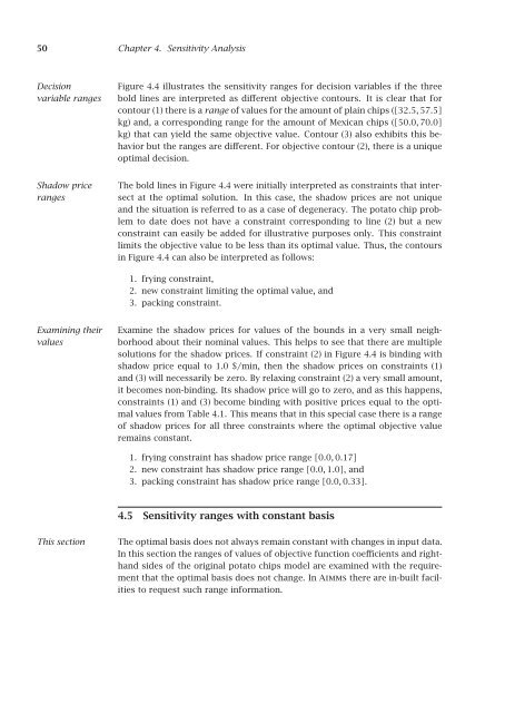
- Page 69: 4.4. Sensitivity ranges with consta
- Page 73 and 74: Chapter 5 Network Flow Models Here,
- Page 75 and 76: 5.2. Example of a network flow mode
- Page 77 and 78: 5.3. Network formulation 57 The fol
- Page 79 and 80: 5.5. Pure network flow models 59 Be
- Page 81 and 82: 5.6. Other network models 61 If the
- Page 83: Part II General Optimization Modeli
- Page 86 and 87: 66 Chapter 6. Linear Programming Tr
- Page 88 and 89: 68 Chapter 6. Linear Programming Tr
- Page 90 and 91: 70 Chapter 6. Linear Programming Tr
- Page 92 and 93: 72 Chapter 6. Linear Programming Tr
- Page 94 and 95: 74 Chapter 6. Linear Programming Tr
- Page 96 and 97: 76 Chapter 6. Linear Programming Tr
- Page 98 and 99: 78 Chapter 7. Integer Linear Progra
- Page 100 and 101: 80 Chapter 7. Integer Linear Progra
- Page 102 and 103: 82 Chapter 7. Integer Linear Progra
- Page 104 and 105: 84 Chapter 7. Integer Linear Progra
- Page 106 and 107: 86 Chapter 7. Integer Linear Progra
- Page 108 and 109: 88 Chapter 7. Integer Linear Progra
- Page 111 and 112: Chapter 8 An Employee Training Prob
- Page 113 and 114: 8.2. Model formulation 93 Minimize:
- Page 115 and 116: 8.3. Solutions from conventional so
- Page 117 and 118: 8.5. Introducing probabilistic cons
- Page 119 and 120: 8.6. Summary 99 Minimize: Subject t
- Page 121 and 122:
9.2. Model formulation 101 each par
- Page 123 and 124:
9.3. Adding logical conditions 103
- Page 125 and 126:
9.3. Adding logical conditions 105
- Page 127 and 128:
9.5. Summary 107 When all elements
- Page 129 and 130:
Chapter 10 A Diet Problem This chap
- Page 131 and 132:
10.2. Model formulation 111 Paramet
- Page 133 and 134:
10.3. Quantities and units 113 To p
- Page 135 and 136:
10.3. Quantities and units 115 Mode
- Page 137 and 138:
Chapter 11 A Farm Planning Problem
- Page 139 and 140:
11.1. Problem description 119 labor
- Page 141 and 142:
11.2. Model formulation 121 the an
- Page 143 and 144:
11.2. Model formulation 123 in the
- Page 145 and 146:
11.3. Model results 125 In Aimms yo
- Page 147 and 148:
Chapter 12 A Pooling Problem In thi
- Page 149 and 150:
12.1. Problem description 129 When
- Page 151 and 152:
12.2. Model description 131 Let f(p
- Page 153 and 154:
12.3. A worked example 133 Due to m
- Page 155 and 156:
12.3. A worked example 135 In this
- Page 157:
Part IV Intermediate Optimization M
- Page 160 and 161:
140 Chapter 13. A Performance Asses
- Page 162 and 163:
142 Chapter 13. A Performance Asses
- Page 164 and 165:
144 Chapter 13. A Performance Asses
- Page 166 and 167:
146 Chapter 13. A Performance Asses
- Page 168 and 169:
148 Chapter 13. A Performance Asses
- Page 170 and 171:
150 Chapter 14. A Two-Level Decisio
- Page 172 and 173:
152 Chapter 14. A Two-Level Decisio
- Page 174 and 175:
154 Chapter 14. A Two-Level Decisio
- Page 176 and 177:
156 Chapter 14. A Two-Level Decisio
- Page 178 and 179:
158 Chapter 14. A Two-Level Decisio
- Page 180 and 181:
160 Chapter 14. A Two-Level Decisio
- Page 182 and 183:
162 Chapter 14. A Two-Level Decisio
- Page 184 and 185:
164 Chapter 15. A Bandwidth Allocat
- Page 186 and 187:
166 Chapter 15. A Bandwidth Allocat
- Page 188 and 189:
168 Chapter 15. A Bandwidth Allocat
- Page 190 and 191:
170 Chapter 15. A Bandwidth Allocat
- Page 192 and 193:
172 Chapter 15. A Bandwidth Allocat
- Page 194 and 195:
174 Chapter 16. A Power System Expa
- Page 196 and 197:
176 Chapter 16. A Power System Expa
- Page 198 and 199:
178 Chapter 16. A Power System Expa
- Page 200 and 201:
180 Chapter 16. A Power System Expa
- Page 202 and 203:
182 Chapter 16. A Power System Expa
- Page 204 and 205:
184 Chapter 16. A Power System Expa
- Page 206 and 207:
Chapter 17 An Inventory Control Pro
- Page 208 and 209:
188 Chapter 17. An Inventory Contro
- Page 210 and 211:
190 Chapter 17. An Inventory Contro
- Page 212 and 213:
192 Chapter 17. An Inventory Contro
- Page 214 and 215:
194 Chapter 17. An Inventory Contro
- Page 216 and 217:
196 Chapter 17. An Inventory Contro
- Page 218 and 219:
198 Chapter 17. An Inventory Contro
- Page 221 and 222:
Chapter 18 A Portfolio Selection Pr
- Page 223 and 224:
18.1. Introduction and background 2
- Page 225 and 226:
18.2. A strategic investment model
- Page 227 and 228:
18.3. Required mathematical concept
- Page 229 and 230:
18.4. Properties of the strategic i
- Page 231 and 232:
18.4. Properties of the strategic i
- Page 233 and 234:
18.5. Example of strategic investme
- Page 235 and 236:
18.6. A tactical investment model 2
- Page 237 and 238:
18.7. Example of tactical investmen
- Page 239 and 240:
18.8. One-sided variance as portfol
- Page 241 and 242:
18.9. Adding logical constraints 22
- Page 243 and 244:
18.10. Piecewise linear approximati
- Page 245 and 246:
18.11. Summary 225 Note that the ab
- Page 247 and 248:
Chapter 19 A File Merge Problem Thi
- Page 249 and 250:
19.1. Problem description 229 No. o
- Page 251 and 252:
19.2. Mathematical formulation 231
- Page 253 and 254:
19.2. Mathematical formulation 233
- Page 255 and 256:
19.4. The simplex method 235 the mo
- Page 257 and 258:
19.5. Algorithmic approach 237 Assu
- Page 259 and 260:
19.6. Summary 239 S and x ij from i
- Page 261 and 262:
Chapter 20 A Cutting Stock Problem
- Page 263 and 264:
20.2. The initial model formulation
- Page 265 and 266:
20.3. Delayed cutting pattern gener
- Page 267 and 268:
20.3. Delayed cutting pattern gener
- Page 269 and 270:
20.4. Extending the original cuttin
- Page 271 and 272:
Chapter 21 A Telecommunication Netw
- Page 273 and 274:
21.2. Bottleneck identification mod
- Page 275 and 276:
21.2. Bottleneck identification mod
- Page 277 and 278:
21.3. Path generation technique 257
- Page 279 and 280:
21.3. Path generation technique 259
- Page 281 and 282:
21.4. A worked example 261 In the a
- Page 283 and 284:
21.5. Summary 263 21.5 Summary In t
- Page 285 and 286:
22.1. Problem description 265 Plant
- Page 287 and 288:
22.3. Solve large instances through
- Page 289 and 290:
22.4. Benders’ decomposition with
- Page 291 and 292:
22.4. Benders’ decomposition with
- Page 293 and 294:
22.6. Formulating dual models 273 T
- Page 295 and 296:
22.7. Application of Benders’ dec
- Page 297 and 298:
22.7. Application of Benders’ dec
- Page 299 and 300:
22.8. Computational considerations
- Page 301 and 302:
22.9. A worked example 281 For each
- Page 303 and 304:
22.10. Summary 283 Exercises 22.1 I
- Page 305:
Part VI Appendices
- Page 308 and 309:
Index Symbols λ-formulation, 84 A
- Page 310 and 311:
290 Index conditional, 81 either-or
- Page 312 and 313:
292 Index simplex iteration, 236 me
- Page 314 and 315:
294 Bibliography [Ch96] A. Charnes,


