On converging shock waves of spherical and polyhedral form
On converging shock waves of spherical and polyhedral form
On converging shock waves of spherical and polyhedral form

You also want an ePaper? Increase the reach of your titles
YUMPU automatically turns print PDFs into web optimized ePapers that Google loves.
372 D. W. Schwendeman<br />
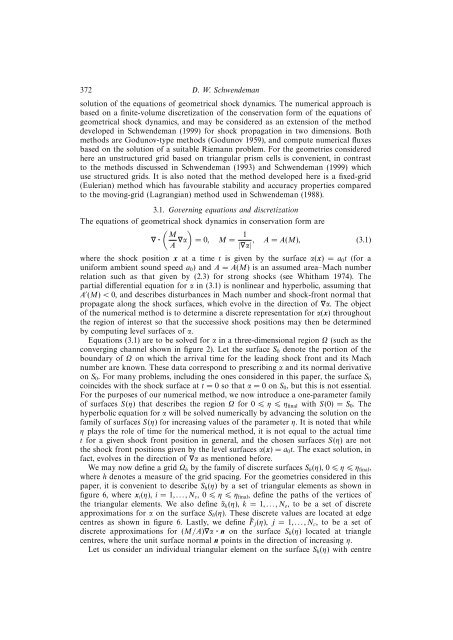
solution <strong>of</strong> the equations <strong>of</strong> geometrical <strong>shock</strong> dynamics. The numerical approach is<br />
based on a finite-volume discretization <strong>of</strong> the conservation <strong>form</strong> <strong>of</strong> the equations <strong>of</strong><br />
geometrical <strong>shock</strong> dynamics, <strong>and</strong> may be considered as an extension <strong>of</strong> the method<br />
developed in Schwendeman (1999) for <strong>shock</strong> propagation in two dimensions. Both<br />
methods are Godunov-type methods (Godunov 1959), <strong>and</strong> compute numerical fluxes<br />
based on the solution <strong>of</strong> a suitable Riemann problem. For the geometries considered<br />
here an unstructured grid based on triangular prism cells is convenient, in contrast<br />
to the methods discussed in Schwendeman (1993) <strong>and</strong> Schwendeman (1999) which<br />
use structured grids. It is also noted that the method developed here is a fixed-grid<br />
(Eulerian) method which has favourable stability <strong>and</strong> accuracy properties compared<br />
to the moving-grid (Lagrangian) method used in Schwendeman (1988).<br />
3.1. Governing equations <strong>and</strong> discretization<br />
The equations <strong>of</strong> geometrical <strong>shock</strong> dynamics in conservation <strong>form</strong> are<br />
( ) M<br />
∇ ·<br />
A ∇α = 0, M = 1 , A = A(M), (3.1)<br />
|∇α|<br />
where the <strong>shock</strong> position x at a time t is given by the surface α(x) = a 0 t (for a<br />
uni<strong>form</strong> ambient sound speed a 0 ) <strong>and</strong> A = A(M) is an assumed area–Mach number<br />
relation such as that given by (2.3) for strong <strong>shock</strong>s (see Whitham 1974). The<br />
partial differential equation for α in (3.1) is nonlinear <strong>and</strong> hyperbolic, assuming that<br />
A ′ (M) < 0, <strong>and</strong> describes disturbances in Mach number <strong>and</strong> <strong>shock</strong>-front normal that<br />
propagate along the <strong>shock</strong> surfaces, which evolve in the direction <strong>of</strong> ∇α. The object<br />
<strong>of</strong> the numerical method is to determine a discrete representation for α(x) throughout<br />
the region <strong>of</strong> interest so that the successive <strong>shock</strong> positions may then be determined<br />
by computing level surfaces <strong>of</strong> α.<br />
Equations (3.1) are to be solved for α in a three-dimensional region Ω (such as the<br />
<strong>converging</strong> channel shown in figure 2). Let the surface S 0 denote the portion <strong>of</strong> the<br />
boundary <strong>of</strong> Ω on which the arrival time for the leading <strong>shock</strong> front <strong>and</strong> its Mach<br />
number are known. These data correspond to prescribing α <strong>and</strong> its normal derivative<br />
on S 0 . For many problems, including the ones considered in this paper, the surface S 0<br />
coincides with the <strong>shock</strong> surface at t = 0 so that α = 0 on S 0 , but this is not essential.<br />
For the purposes <strong>of</strong> our numerical method, we now introduce a one-parameter family<br />
<strong>of</strong> surfaces S(η) that describes the region Ω for 0 η η final with S(0) = S 0 . The<br />
hyperbolic equation for α will be solved numerically by advancing the solution on the<br />
family <strong>of</strong> surfaces S(η) for increasing values <strong>of</strong> the parameter η. It is noted that while<br />
η plays the role <strong>of</strong> time for the numerical method, it is not equal to the actual time<br />
t for a given <strong>shock</strong> front position in general, <strong>and</strong> the chosen surfaces S(η) are not<br />
the <strong>shock</strong> front positions given by the level surfaces α(x) = a 0 t. The exact solution, in<br />
fact, evolves in the direction <strong>of</strong> ∇α as mentioned before.<br />
We may now define a grid Ω h by the family <strong>of</strong> discrete surfaces S h (η), 0 η η final ,<br />
where h denotes a measure <strong>of</strong> the grid spacing. For the geometries considered in this<br />
paper, it is convenient to describe S h (η) by a set <strong>of</strong> triangular elements as shown in<br />
figure 6, where x i (η), i = 1, . . . , N v , 0 η η final , define the paths <strong>of</strong> the vertices <strong>of</strong><br />
the triangular elements. We also define ˜α k (η), k = 1, . . . , N e , to be a set <strong>of</strong> discrete<br />
approximations for α on the surface S h (η). These discrete values are located at edge<br />
centres as shown in figure 6. Lastly, we define ˜F j (η), j = 1, . . . , N c , to be a set <strong>of</strong><br />
discrete approximations for (M/A)∇α · n on the surface S h (η) located at triangle<br />
centres, where the unit surface normal n points in the direction <strong>of</strong> increasing η.<br />
Let us consider an individual triangular element on the surface S h (η) with centre


![MATH 1500 Sample Questions Exam 2 1. [3.7] A 10-ft plank is ...](https://img.yumpu.com/43861920/1/190x245/math-1500-sample-questions-exam-2-1-37-a-10-ft-plank-is-.jpg?quality=85)