% MATLAB script file implementing the method of steepest descent ...

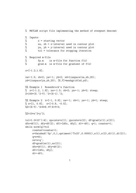
% MATLAB script file implementing the method of steepest descent% Inputs:% x = starting vector% xa, xb = x-interval used in contour plot% ya, yb = y-interval used in contour plot% tol = tolerance for stopping iteration% Required m-file% fp.m is m-file for function f(x)% grad.m is m-file for gradient of f(x)x=[-1.2;1.8];xa=-1.5; xb=2; ya=-1; yb=2; xd=linspace(xa,xb,20);yd=linspace(ya,yb,20); [X,Y]=meshgrid(xd,yd);%% Example 1 Rosenbrock’s function% x=[-1.2, 1.8]; xa=-1.5; xb=2; ya=-1; yb=2; steep;Z=100*(X.^2-Y).^2+(X-1).^2;%% Example 2 x=[-1, 0.8]; xa=-1; xb=1; ya=-1; yb=1; steep;% x=[1, 0.8]; x=[-0.8, -0.5];%Z=(X-Y).^4+8*X.*Y-X+Y+3;%Z=10*x^2+y^2;tol=1.0*10^(-4); xpoints=x(1); ypoints=x(2); df=grad(x(1),x(2));dfx=df(1); dfy=df(2); df1=[dfx, dfy]; d1=-df1; q=1; counter=1;while norm(q)>tolcounter=counter+1;s=fminbnd(’fp’,0,1,optimset(’TolX’,0.00001),x(1),x(2),d1(1),d1(2));q=s*d1;xx=x+q’;df=grad(xx(1),xx(2));dfx=df(1); dfy=df(2);df1=[dfx, dfy];d1=-df1;1

x=xx;% fprintf(’\n %i Computed Solution = %e %e’,counter,x);end;xpoints=[xpoints, x(1)];ypoints=[ypoints, x(2)];hold oncontour(X,Y,Z,30,’b’)plot(xpoints,ypoints,’ko-’)hold offpauseerror=sqrt((1-x(1))^2+(1-x(2))^2);fprintf(’\n %i Computed Solution = %e %e Error = %e’,counter,x,error);2