University of Trento Automatic Control 1: Solutions Exercise 1 (15 ...
University of Trento Automatic Control 1: Solutions Exercise 1 (15 ...
University of Trento Automatic Control 1: Solutions Exercise 1 (15 ...

Create successful ePaper yourself
Turn your PDF publications into a flip-book with our unique Google optimized e-Paper software.
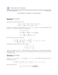
<strong>University</strong> <strong>of</strong> <strong>Trento</strong><br />
Pr<strong>of</strong>. Alberto Bemporad April 22, 2010<br />
<strong>Automatic</strong> <strong>Control</strong> 1: <strong>Solutions</strong><br />
<strong>Exercise</strong> 1 (<strong>15</strong> points)<br />
The system equations are<br />
{<br />
A1 ḣ 1 (t) = −(a 12 + a 13 ) √ 2gh 1 (t) + ϕ(t)<br />
A 2 ḣ 2 (t) = −a 23<br />
√<br />
2gh2 (t) + a 12<br />
√<br />
2gh1 (t)<br />
Introducing the state and output variables as x 1 = h 1 , x 2 = h 2 , u = ϕ = u, y = h 2 , we obtain a state-space<br />
representation with ⎧ √ ⎪⎨ ẋ 1 (t) = − a12+a13<br />
A 2gx1<br />
1<br />
(t) + u(t)<br />
√ √A 1<br />
ẋ<br />
⎪ 2 (t) = − a23<br />
⎩<br />
A 2gx2<br />
2<br />
(t) + a12<br />
A 2gx1<br />
2<br />
(t)<br />
y(t) = x 2 (t)<br />
Substituting a 12 = a 23 = a 13 = 1 m 2 , A 1 = 200 m 2 , A 2 = 100 m 2 , g = 10, it yields<br />
{<br />
ẋ 1 (t) = − √ √<br />
20<br />
100 x1 (t) + u(t)<br />
200<br />
ẋ 2 (t) = − √ √<br />
20<br />
100 x2 (t) + √ √<br />
20<br />
100 x1 (t)<br />
Solving ẋ 1 = ẋ 2 = 0 with ū = 10, it yields<br />
Linearizing around these values, we obtain<br />
[<br />
]<br />
A =<br />
− ga13a23(a12+a13)<br />
a 12ūA 2<br />
− g(a12+a13)2<br />
ūA 1<br />
0<br />
ga 12(a 12+a 13)<br />
ūA 2<br />
=<br />
¯x 1 = ¯x 2 = 5/4<br />
[<br />
−<br />
1<br />
50<br />
0<br />
1<br />
50<br />
− 1 50<br />
] [ 1<br />
, B = 200<br />
0<br />
]<br />
, C = [ 0 1 ] , D = 0<br />
The eigenvalues <strong>of</strong> matrix A are the elements on the diagonal, which have a strictly negative real part.<br />
Therefore, the linearized system is asymptotically stable. Finally, the observability matrix is<br />
[ 1<br />
]<br />
R = 200<br />
− 1<br />
10000<br />
1<br />
0<br />
10000<br />
which is full rank.<br />
stabilizable.<br />
<strong>Exercise</strong> 2 (13 points)<br />
Therefore the system is completely reachable and, <strong>of</strong> consequence, controllable and<br />
[ ] 0 1<br />
As for the first request, the reachability matrix is R = which is full rank, making it possible to<br />
1 3<br />
to place the poles <strong>of</strong> the closed-loop system (A + BK) at any desired position. Given the controller gain<br />
K = [k 1 k 2 ], the characteristic polynomial is<br />
([ ])<br />
λ − 2 −1<br />
p c (λ) = det(I − (A + BK)) = det<br />
= λ 2 + (−k<br />
1 − k 1 λ − 3 − k 2 − 5)λ − k 1 + 2k 2 + 7<br />
2
The desired characteristic polynomial is p d (λ) = (λ + 2) 2 = λ 2 + 4λ + 4. Forcing the equalities between<br />
the coefficients <strong>of</strong> the two polynomials, it yields k 1 = −<strong>15</strong> and k 2 = −9. The controller is then u(t) =<br />
−9x 1 (t) − <strong>15</strong>x 2 (t).<br />
[ ] 1 1<br />
As for the second request, the observability matrix is Θ = which is full rank, and then it is possible<br />
1 4<br />
to place the poles <strong>of</strong> the observer at will. Given an observer gain L = [l 1 l 2 ] ′ , the characteristic polynomial<br />
can be expressed as<br />
([ ])<br />
λ − 2 + l1 l<br />
p c (λ) = det(I − (A − LC)) = det<br />
1 − 1<br />
= λ 2 + (l<br />
1 + l 2 λ − 3 + l 1 + l 2 − 5)λ − 4l 1 − l 2 + 7<br />
2<br />
The desired characteristic polynomial is p d (λ) = (λ + 1)(λ + 2) = λ 2 + 3λ + 2. Forcing the equalities between<br />
the coefficients <strong>of</strong> the two polynomials, it yields l 1 = −1 and l 2 = 9. The resulting Luenberger observer is<br />
[<br />
] [ ] [ ]<br />
3 2<br />
0 −1<br />
ˆx(t) =<br />
ˆx(t) + u(t) + y(t)<br />
−10 −6<br />
1<br />
9<br />
Placing the poles at (0.5, 0.5) is possible, because the system is completely observable. This would imply an<br />
unstable dynamics <strong>of</strong> the observation error, which would diverge to infinity, making the observer useless.<br />
<strong>Exercise</strong> 3 (5 points)<br />
For the Laplace transform F (s) <strong>of</strong> a continuous-time function f(t):<br />
• Initial value theorem: lim t→0 + f(t) = lim s→∞ sF (s)<br />
• Final value theorem: lim t→+∞ f(t) = lim s→0 sF (s)<br />
For the Zeta transform F (z) <strong>of</strong> a function f(k):<br />
• Initial value theorem: f(0) = lim z→∞ F (z)<br />
• Final value theorem: lim k→+∞ f(k) = lim z→1 (z − 1)F (z)