PDF 49k - Ministry of Forests
PDF 49k - Ministry of Forests
PDF 49k - Ministry of Forests

Create successful ePaper yourself
Turn your PDF publications into a flip-book with our unique Google optimized e-Paper software.
PAMPHLET NO. # 13 DATE: November 28, 1988<br />
SUBJECT:<br />
Analysis <strong>of</strong> Covariance: Comparing Adjusted Means<br />
Comparisons between adjusted means from an analysis <strong>of</strong> covariance (ANCOVA) are <strong>of</strong>ten<br />
desired if the overall F-test for treatment effects is significant. As in ANOVA, specific questions<br />
about the means should be tested with contrasts, while a general question <strong>of</strong> "where do the<br />
differences lie?" can be tested by multiple pair-wise comparisons (similar to Duncan's MRT or<br />
Fisher's protected LSD test for ANOVA).<br />
Suppose that the response variable is Y, the treatment variable is A, and the covariate is X.<br />
The calculations require two SAS runs:<br />
i) ANOVA on the covariate, X with treatment A<br />
ii) ANCOVA on Y with treatment A and covariate X<br />
which produces output for the following tables:<br />
i) ANOVA on X<br />
Source <strong>of</strong> Degrees <strong>of</strong> Sums <strong>of</strong> Mean<br />
Variation Freedom Squares Square<br />
��������������������� ������������������������� ����������������� ���������������<br />
Treatment A a-l SSBX MSBX<br />
Error ∑ni-a SSEX MSEX<br />
ii) ANCOVA on Y<br />
Source <strong>of</strong> Degrees <strong>of</strong> Sums <strong>of</strong> Mean<br />
Variation Freedom Squares Square<br />
��������������������� ������������������������� ����������������� ���������������<br />
Treatment A a-l SSBY MSBY<br />
Covariate X l SSX MSX<br />
Error ∑ni-a-l SSEY MSEY<br />
Where a is the number <strong>of</strong> levels for treatment A and ni is the sample size per treatment level.<br />
l. CONTRASTS--DUNN-BONFERRONI TESTS<br />
Contrasts are calculated the usual way but on adjusted means (obtained with the LSMEANS<br />
statements in PROC GLM) instead <strong>of</strong> the ordinary, unadjusted means. That is, a contrast<br />
� ��� ���<br />
γ = ∑ ci Yiadj, where ci are the usual contrast coefficients and Yiadj are the adjusted means. The<br />
standard error <strong>of</strong> the contrast is calculated by:<br />
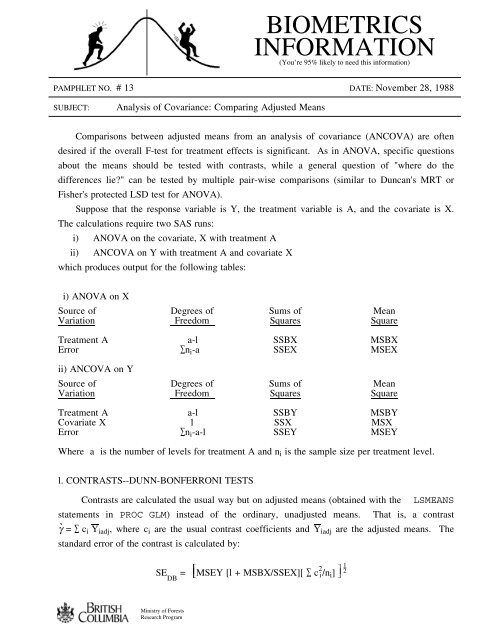
BIOMETRICS<br />
INFORMATION<br />
(You’re 95% likely to need this information)<br />
� 2 ��<br />
SE = ˜MSEY [l + MSBX/SSEX][ ∑ ci/ni] <br />
DB<br />
<strong>Ministry</strong> <strong>of</strong> <strong>Forests</strong><br />
Research Program
The Dunn-Bonferroni t-test is calculated by:<br />
2<br />
�<br />
t = γ /SE with df = ∑ni -a-l<br />
DB DB<br />
NOTE: The critical values for this test are NOT those <strong>of</strong> the usual t-distribution. Table A.6 <strong>of</strong><br />
Huitema is one source <strong>of</strong> the appropriate values.<br />
2. MULTIPLE PAIRWISE COMPARISONS--PAIRWISE LSD TEST<br />
This test is ONLY conducted if the F-test for the treatment, A, is significant. The numerator<br />
��� ���<br />
<strong>of</strong> the t-test is simply the difference between a specific pair <strong>of</strong> means, Yiadj - Yjadj while the<br />
denominator is the standard error <strong>of</strong> the difference given by:<br />
� ��� ��� ��<br />
SE = � MSEY [1/ni +1/nj) +(Xi -Xj) 2 /SSEX] �<br />
˜ <br />
��� ���<br />
The (ordinary) t-value is calculated by t = (Yiadj -Yjadj)/SE with df = ∑ ni -a-1. Theα-level for<br />
the t-test should be the same as that <strong>of</strong> the overall F-test.<br />
EXAMPLE: Data from Table 3.l (page 38) <strong>of</strong> Huitema.<br />
A=1 A=2 A=3<br />
������������������������������������������������������������ ��������������������������������������������������������������� ���������������������������������������������������������������<br />
X=29 Y=15 X=47 Y=39 X=22 Y=20 X=43 Y=44 X=33 Y=14 X=48 Y=42<br />
49 19 46 23 24 34 64 46 45 20 63 40<br />
48 21 74 38 49 28 61 47 35 30 57 38<br />
35 27 72 33 46 35 55 40 39 32 56 54<br />
53 35 67 50 52 42 54 54 36 34 78 56<br />
������������������������������������������������������������ ��������������������������������������������������������������� ���������������������������������������������������������������<br />
SUMMARY:<br />
�������������������������<br />
CONTRASTS:<br />
���������������������������<br />
Adjusted Means Covariate Means<br />
������������������������������������ �������������������������������������<br />
A=l 28.479 52.0 MSBX = 63.333<br />
A=2 40.33l 47.0 SSEX = 5700<br />
A=3 36.l90 49.0 MSEY = 64.640<br />
-28.479 + 0 + 36. l90<br />
����������������������������������������������������������������������������������������<br />
�������������������������������������������������������������������������������������<br />
LINEAR: t = �<br />
DB � 64.45 [l + 63. 333/5700] [2/10]<br />
= 2.l3, df = 26 prob > 0.05
(28. 479 - 2(40. 33l) + 36. l90)<br />
�����������������������������������������������������������������������������������������<br />
��������������������������������������������������������������������������������������<br />
QUADRATIC: t = �<br />
DB � 64. 64 [1 + 63. 333/5700] [6/10]<br />
PROTECTED LSD TESTS:<br />
�����������������������������������������������������������<br />
3 Pamphlet #13<br />
���������������������������������<br />
= 2.55, df = 26 prob < 0.05, Bonferroni Critical Value is 2.379<br />
28. 479 - 40.33l<br />
����������������������������������������������������������������������������������������<br />
A=1vs A=2: t = ����������������������������������������������������������������������������������<br />
�<br />
� 64.64 [2/10 + (52 - 47) 2 /5700]<br />
= -3.26, DF = 26, prob = 0.003<br />
28.479 - 36.l90<br />
�������������������������������������������������������������������������������������<br />
A=1vs A=3: t = �������������������������������������������������������������������������������<br />
�<br />
� 64.64 [2/10 + (52 - 49) 2 /5700]<br />
= -2.14, df = 26, prob = 0.042<br />
40.33l - 36.l90<br />
����������������������������������������������������������������������������������������<br />
A=2vs A=3: t = ����������������������������������������������������������������������������������<br />
�<br />
2<br />
� 64.64 [2/10 + (52 - 49) /5700]<br />
= 1.15, df = 26, prob = 0.26<br />
THEREFORE: A = 2 3 l<br />
40. 33l 36. l90 28. 479<br />
_______________________________________<br />
NOTE: The CONTRAST statement in PROC GLM produced F-values equal to the square <strong>of</strong> the<br />
above t-values, although the probability levels were substantially different. The output <strong>of</strong><br />
the LSMEANS statement with the PDIFF option were identical to the protected LSD tests<br />
above.<br />
Reference:<br />
Huitema, Bradley, E., l980, The Analysis <strong>of</strong> Covariance and Alternatives, John Wiley and Sons,<br />
Toronto.<br />
CONTACT: Wendy Bergerud<br />
387-5676