Varian Fluorimeter Cary Eclipse

VARIAN FLUORIMETER
CARY ECLIPSE
INITIALIZING THE INSTRUMENT:
• Turn on the computer and turn on the instrument power switch located on its right front
corner. Start the software by double-clicking on the SCAN icon on the desktop.
• Once the instrument is initialized, the screen should have the Start and Stop buttons at
the top center. If Connect appears in place of Start, press Connect in order bring the
instrument online.
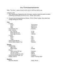
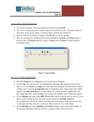
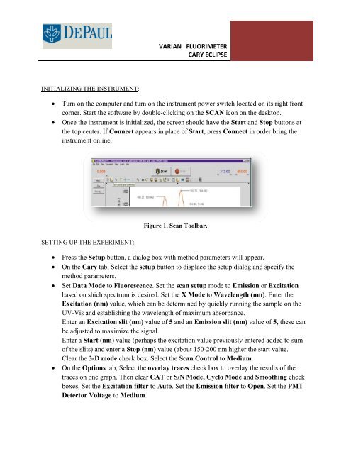
SETTING UP THE EXPERIMENT:
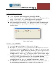
Figure 1. Scan Toolbar.
• Press the Setup button, a dialog box with method parameters will appear.
• On the Cary tab, Select the setup button to displace the setup dialog and specify the
method parameters.
• Set Data Mode to Fluorescence. Set the scan setup mode to Emission or Excitation
based on shich spectrum is desired. Set the X Mode to Wavelength (nm). Enter the
Excitation (nm) value, which can be determined by quickly running the sample on the
UV-Vis and establishing the wavelength of maximum absorbance.
Enter an Excitation slit (nm) value of 5 and an Emission slit (nm) value of 5, these can
be adjusted to maximize the signal.
Enter a Start (nm) value (perhaps the excitation value previously entered added to sum
of the slits) and enter a Stop (nm) value (about 150-200 nm higher the start value.
Clear the 3-D mode check box. Select the Scan Control to Medium.
• On the Options tab, Select the overlay traces check box to overlay the results of the
traces on one graph. Then clear CAT or S/N Mode, Cyclo Mode and Smoothing check
boxes. Set the Excitation filter to Auto. Set the Emission filter to Open. Set the PMT
Detector Voltage to Medium.

• On the Reports tab, enter Operator Name. To automatically label peaks on the
spectrum, select Maximum Peak or All Peaks options. The peak threshold limit and
labeling options are altered by pressing the Peak Information button.
• On the Auto Storage tab, select whether to save the scans before or after a run. Selecting
after the run (not the default choice) will avoid saving bad data.
DATA COLLECTION:
Figure 2. Set up Dialog Box.
• In order to zero the instrument, place the blank solution in the sample compartment #4.
Press the zero button to zero the system. When the result is zeroed, the word ‘Zeroed’
will appear in the Y display box in the top left corner of the scan application window.
DO NOT discard the blank, you must zero the system before each reading.
• Replace the blank with the sample to be analyzed in compartment #4 and press the Start
button. You will be asked for a sample name then the spectrum will start running and the
trace will appear in the graphics area. Autoscale the spectrum if it goes offscale. Once
the run is completed, a save file box will be presented to allow naming the file. Any peak
information will be printed in the report box (the bottom half underneath the plot).
• Text can be added to the plot by pressing the A button. When running multiple scans in
one session, pressing the traces button (the farthest left button in the toolbar) to select
individual data sets can be selected and made visible in the current plot. Please note that
all data plots (including any baselines) are still accessible through the Graph menu, and
all will be printed out when printing the data. In order to omit any data set, right click on
the graph with that data and select Remove Graph.
2

• In order to manually mark a certain point on a spectrum, right click at that point and
select Print x-y Point. The coordinates will be printed in the report window. Text can be
added or changed in the report window by selecting Edit Report on the Edit menu and
manipulating the text as needed. Double clicking on the report window will allow to
expand it to full size.
• To save the session as-is, including the report window contents and alterations made to
the scans, select Save Data As… from the File menu and enter the name for the batch
file. In order to export some of the data for use in other programs, click on the graph of
that data, select Save Data As…from the File menu, and select Spreadsheet ascii
(*.CSV) from the Save Files As box.
Figure 3. Peak Labels.
• Once the plot has been drawn, you may use the cursor mode to switch between Free
mode and Track Mode in order to monitor the X and Y values by dragging the
intersecting lines along the graph to the point of interest.
SIMPLE READS:
• This feature allows for sample analysis at one wavelength. Access the Simple Reads icon
from the Cary Eclipse folder and click on Setup.
• Set up the experiment in the same manner as in the Scan mode.
• Proceeds to zero the instrument and press on Read to begin collecting data.
CONCENTRATION:
• This feature allows for sample analysis at one wavelength. Access the Simple Reads icon
from the Cary Eclipse folder and click on Setup.
• Set up the experiment in the same manner as in the Scan mode.
3

• In the Standards tab enter the desired Unit Selection. Enter the number standard
samples to be analyzed. In Replicates enter one less than the standard sample number.
Clear the Std. Averaging option and enter the various concentrations in the appropriate
boxes.
• In the Fit Type tab highlight the type of fit appropriate for the data and adjust the fit by
altering the default of 0.9500 R 2 in Min R 2 .
• In the Samples tab enter the Number of Samples and Replicates and label samples.
• In order to run the standards and samples, zero the instrument and select the samples to
be used for calibration from the Standard/Sample selection. Available samples can be
Selected for Analysis by using the arrows.
• Click and foow the on screen direction in order to Present Standard to be analyzed.
Once all standards are analyzed a calibration curve with be automatically displayed.
Figure 4. Sample Selection.
• Sample analysis is analogous to standards.
Figure 5. Sample Concentration Results.
4