Variable Baseline/Resolution Stereo

Variable Baseline/Resolution Stereo
David Gallup 1 , Jan-Michael Frahm 1 , Philippos Mordohai 2 , Marc Pollefeys 1,3
1 University of North Carolina 2 University of Pennsylvania 3 ETH Zurich
Chapel Hill, NC Philadelphia, PA Zurich, Switzerland
{gallup, jmf}@cs.unc.edu, mordohai@seas.penn.edu, marc.pollefeys@inf.ethz.ch
Abstract
We present a novel multi-baseline, multi-resolution
stereo method, which varies the baseline and resolution proportionally
to depth to obtain a reconstruction in which the
depth error is constant. This is in contrast to traditional
stereo, in which the error grows quadratically with depth,
which means that the accuracy in the near range far exceeds
that of the far range. This accuracy in the near range is
unnecessarily high and comes at significant computational
cost. It is, however, non-trivial to reduce this without also
reducing the accuracy in the far range. Many datasets, such
as video captured from a moving camera, allow the baseline
to be selected with significant flexibility. By selecting an appropriate
baseline and resolution (realized using an image
pyramid), our algorithm computes a depthmap which has
these properties: 1) the depth accuracy is constant over the
reconstructed volume, 2) the computational effort is spread
evenly over the volume, 3) the angle of triangulation is held
constant w.r.t. depth. Our approach achieves a given target
accuracy with minimal computational effort, and is orders
of magnitude faster than traditional stereo.
1. Introduction
Stereo is a well-studied problem in computer vision [14].
Recent work has been very successful in solving the correspondence
problem, which is to decide which pixels in one
image correspond to which pixels in another. Techniques
employing graph cuts and belief propagation can achieve
error rates of less than 1% (on laboratory data). However,
for many applications the goal is ultimately not pixel correspondence
but depth accuracy. Even with perfect correspondences,
the depth error in traditional stereo grows
quadratically with depth, which means that the accuracy in
the near range far exceeds that of the far range. While the
accuracy in the far range is unusably bad, the accuracy in
the near range is unnecessarily high and comes at significant
computational cost. Accuracy can be improved by incorporating
multiple views. These views provide additional
information which aids in the correspondence problem, but
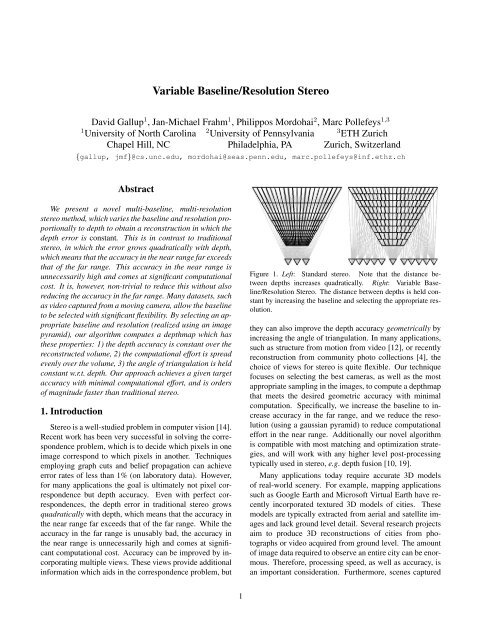
Figure 1. L eft: Standard stereo. Note that the distance between
depths increases quadratically. R ight: V ariable B aseline/Resolution
Stereo. The distance between depths is held constant
by increasing the baseline and selecting the appropriate resolution.
they can also improve the depth accuracy geometrically by
increasing the angle of triangulation. In many applications,
such as structure from motion from video [12 ], or recently
reconstruction from community photo collections [4], the
choice of views for stereo is quite fl exible. O ur technique
focuses on selecting the best cameras, as well as the most
appropriate sampling in the images, to compute a depthmap
that meets the desired geometric accuracy with minimal
computation. Specifically, we increase the baseline to increase
accuracy in the far range, and we reduce the resolution
(using a gaussian pyramid) to reduce computational
effort in the near range. Additionally our novel algorithm
is compatible with most matching and optimization strategies,
and will work with any higher level post-processing
typically used in stereo, e.g. depth fusion [10 , 19 ].
Many applications today require accurate 3 D models
of real-world scenery. For example, mapping applications
such as Google Earth and Microsoft V irtual Earth have recently
incorporated textured 3 D models of cities. These
models are typically extracted from aerial and satellite images
and lack ground level detail. Several research projects
aim to produce 3 D reconstructions of cities from photographs
or video acquired from ground level. The amount
of image data required to observe an entire city can be enormous.
Therefore, processing speed, as well as accuracy, is
an important consideration. Furthermore, scenes captured
1

from ground level typically exhibit a large depth range.
Standard stereo is ill-suited to such scenes since the error
grows quadratically with depth.
The motivation for our approach derives from the point
of view of a system designer wishing to employ stereo as a
measuring device. O ften, the definition of the stereo problem
assumes the camera parameters are given and fixed,
but these parameters have a significant effect on the depth
accuracy of stereo. The system designer has some accuracy
requirements in mind and, with traditional stereo
methods, must carefully select baseline, focal length, and
field of view in order to meet these requirements. Furthermore,
computation time is important in real systems,
and so the designer must be conservative. It is unacceptable
to spend large amounts of time obtaining accuracy that
far exceeds the minimum requirement. B alancing accuracy
and efficiency for standard stereo is difficult indeed
due to its quadratic error characteristics. O ur novel algorithm
enhances stereo to be able to efficiently use the additional
information contained in dense image sets such as
video by dynamically selecting the appropriate baseline and
image scale for each depth estimate. In contrast to traditional
stereo our technique guarantees a constant target accuracy
throughout the maximal possible volume with orders
of magnitude less computational effort.
1.1. Variable Baseline/Resolution Stereo
The motivation for our algorithm is derived from the
depth error in stereo, which can be shown to be
ɛ z = z2
bf · ɛ d (1)
where ɛ z is the depth error, z is the depth, b is the baseline,
f is the focal length of the camera in pixels, and ɛ d is the
matching error in pixels (disparity values). Dense image
sets, such as video, allow the baseline b to be selected with
great fl exibility, and because f is measured in pixels, the
focal length can be varied by selecting the appropriate scale
in a gaussian pyramid (up to the maximum value of f at
full resolution). The principal idea of our algorithm is to set
both b and f proportionally to z throughout the depthmap
computation, thereby canceling the quadratic z term, and
leaving ɛ z constant w.r.t. depth. Thus matching scores for
depths in the near range are computed using a narrow baseline
and coarse resolution, while depths in the far range use
a wider baseline and finer resolution.
O ur algorithm, which we call V ariable B aseline/Resolution
Stereo, exhibits three important properties:
1. B y selecting the baseline and resolution proportionally
to the depth, we can match the quadratic term in the
depth error, and achieve constant accuracy over the reconstructed
volume.
2 . B ecause the accuracy is constant throughout the reconstructed
volume, the computational effort is also
evenly spread throughout the volume.
3 . The baseline grows linearly with depth, therefore the
angle of triangulation remains constant 1 .
To the best of our knowledge, our method is the first to exhibit
all three properties.
In the following sections we consider previous work, analyze
the error and time complexity of our algorithm as
compared to traditional stereo, discuss the implementation
of our algorithm in detail, and present results.
2 . P rev ious W ork
Early research on multi-baseline stereo includes the
work of O kutomi and K anade [11] who use both narrow and
wide baselines, which offer different advantages, from a set
of cameras placed on a straight line with parallel optical
axes. A layer-based approach that can handle occlusion and
transparency was presented by Szeliski and Golland [16 ].
The number of layers, however, is hard to estimate a priori
and initialization of the algorithm is difficult. K ang et
al [6 ] explicitly address occlusion in multi-baseline stereo.
For each pixel of the reference view a subset of the cameras
with the minimum matching cost is selected under the
assumption that the pixel may be occluded in the other images.
We also use this scheme in our approach. Sato et al.
[13 ] address video-based 3 D reconstruction using hundreds
of frames for each depth map computation. The median
SSD between the reference and all target views is used for
robustness against occlusions. In general, using multiple
images improves matching, and employing wider baselines
can increase the depth accuracy. O ur approach is unique in
that we use a different set of images throughout the computation
such that the baseline grows proportionally to depth.
Multi-resolution approaches are used for stereo to either
speed up computation or to combine the typically less ambiguous
detection at coarse resolution with the higher precision
of fine resolution. The latter was the motivation for
the approach of Falkenhagen [3 ] in which disparities are
propagated and refined as processing moves from coarse to
fine levels of image pyramids. Y ang and Pollefeys [18 ] presented
an algorithm in which cost functions from several
different resolutions were blended to take advantage of the
reduced ambiguity coming from matching at coarse levels
of the image pyramids and the increased precision coming
from matching at fine levels. K och et al. [7 ] use a multiresolution
stereo algorithm to approximately detect the surfaces
quickly, since processing speed is important for large
scale reconstruction systems which operate on large disparity
ranges. Reducing image resolution results in an equiv-
1 The angle of triangulation is constant w.r.t. to depth. It varies slightly
from pixel to pixel.

alent reduction of the disparity range. Sun [15 ] presented
a method that aims at improving both the speed and reliability
of stereo. It operates in bottom-up fashion on an image
pyramid in which stripes are adaptively merged to form
rectangular regions based on disparity similarity. A twostage
dynamic programming optimization stage produces
the final depth map. In these approaches, multiple resolutions
are used for speed and/or improved matching, but
depth accuracy is not addressed. A key component of our
algorithm is that we use different resolutions at different
depths. Specifically, we use lower resolutions to estimate
depths in the near range in order to avoid unnecessary computations
for accuracy that far exceeds what is required.
Algorithms that take geometric uncertainty explicitly
into account include [9 ] and [7 ]. Matthies et al. [9 ] introduced
an approach based on K alman filtering that estimates
depth and depth uncertainty for each pixel using monocular
video inputs. These estimates are refined incrementally as
more frames become available. K och et al. [7 ] proposed
a similar approach that computes depth maps using pairs
of consecutive images. Support for each correspondence in
the depth maps is found by searching adjacent depth maps
both forward and backward in the sequence. When a match
is consistent with a new camera, the camera is added to
the chain that supports the match. The position of the reconstructed
3 D point is updated using the wider baseline.
While these methods are successful in reducing the error in
the reconstruction, they do not exhibit the properties from
Section 1.1. In particular, the computational effort is concentrated
in the near range, and as a result the depth accuracy
in the near range exceeds that of the far range.
3 . Analy sis
B efore analyzing the accuracy and time complexity of
our stereo algorithm, we shall briefl y address the issue of
depth sampling. Stereo seeks to determine the depth of the
surface along the rays passing through each pixel in a reference
image. Each point along the ray is projected into
any number of target images, and a measure of photoconsistency
is computed. This defines a function in depth, the
minimum (or maximum) of which indicates the depth of the
surface and is discovered by sampling the function at various
depths. The number and location of the samples should
be defined by the pixels in the target images (disparities).
While supersampling can obtain a more accurate minimum,
the minimum itself does not necessarily accurately locate
the surface. B ecause the frequency content of the images
is limited by the resolution, the photoconsistency function
is also limited, and thus the surface can only be localized
to within one pixel. (Sub-pixel accuracy up to 1/4 pixel
is possible, but the depth accuracy is still proportional to
the pixels.) Note also that subsampling the function without
properly filtering the images will lead to aliasing, and
the minimum of the aliased function can often be far from
the minimum of the original function. Therefore the sampling
rate must be on the order of one pixel. In stereo, one
cannot expect to obtain greater depth accuracy simply by
finer disparity sampling, and in order to use coarser sampling
(to reduce computation time and accuracy), filtered
lower-resolution images must be used. For more details on
sampling in stereo, see [17 ].
3 .1. Accuracy and T im e C om p lex ity
We now analyze the time complexity of traditional stereo
and compare it to the time complexity of our variable baseline/resolution
algorithm. O ur analysis assumes that the
cameras are separated by lateral translation and no rotation,
so that all cameras share a common image plane, and pixel
correspondences have the same vertical image coordinate.
This setup, which is convenient for analysis, can be somewhat
relaxed in the actual implementation of our algorithm.
In our analysis we assume that the system designer specifies
a desired accuracy: a maximum error ɛ z , and a maximum
range z f a r . Stereo is expected to deliver depth measurements
with error less than ɛ z for all depths z ≤ z f a r .
Consider two cameras with focal length f separated by
distance b. L et d be the difference in x coordinates, called
disparity, of two corresponding pixels. The depth z of the
triangulated point is given by z = bf d
(where f is measured
in pixels). The depth error can be written in terms of the
disparity error ɛ d :
ɛ z = bf d −
bf =
z2 ɛ d
≈
d + ɛ d bf + zɛ d
z2
bf
· ɛ d . (2 )
The final step is obtained by taking the first order taylor
series approximation about ɛ d = 0.
Here we separate the error into two factors: correspondence
error, ɛ d , and geometric resolution, z 2 /(bf). Geometric
resolution describes the error in terms of the geometry
of the stereo setup, namely baseline, focal length,
and depth. We see that geometric resolution is quadratic
in depth. Correspondence error describes the error from incorrect
matches and the sub-pixel accuracy of the correct
matches. In stereo, correspondence error depends on image
noise, scene texture, and other scene properties such as
occlusions and non-L ambertian surfaces. In this paper we
focus on geometric resolution, and assume that the number
of incorrect matches is reasonably low, and that matching
accuracy is bounded to within one pixel. Therefore, meeting
our target error bound ɛ z at depth z ≤ z f a r depends on
the baseline and focal length of the cameras.
We will now analyze the effect of baseline and focal
length separately, then combined, followed by an analysis
of our algorithm. We focus our analysis on the target accuracy
parameters ɛ z and z f a r .

z depends on b, and b grows quadratically with z ,
Fixed-baseline stereo. For a fixed-baseline stereo system,
where the overlap begins is z n ear =
b
ta n θ f o v /2 . B ecause with z. The baseline is chosen as B(z/z far ), and the reso-
the accuracy can be adjusted by varying the focal
n ear far
there is a point at which z n ear surpasses z far , meaning that
length parameter f. Since f here is measured in pixels, the depth where the target accuracy is met is no longer in
it can be increased either by narrowing the field of view
(zoom), or by increasing the resolution of the sensor. We
assume the field of view θ f o v has been carefully chosen for
the application, meaning f describes the resolution as
the overlapping field of view. In general, one cannot rely on
increasing the baseline alone to meet the target accuracy.
V ariable baseline and resolu tion. In order to avoid z n ear
surpassing z far , the baseline cannot grow faster than linearly
with z far . Thus we set b = βz far where β can be cho-
w = 2f ta n θ f o v
h = w 2 a , (3 ) sen to give a certain angle of triangulation at z far . Given
this constraint, we solve for the resolution needed to meet
where w, h and a are the width, height and aspect ratio of the target accuracy as follows:
the image. We can determine the resolution needed to meet
the target accuracy by solving for f in equation (2 ). (Here
f = z far 2
= z far
(7 )
bɛ z βɛ z
we have assumed ɛ d = 1.)
f = z far 2
number of pixels = z far 2 4 ta n 2 θ fo v
2
ɛ
2
(4)
z β 2 . (8 )
a
bɛ z
From this equation we see that the baseline and the focal
number of pixels = wh = w2
length both grow linearly with z far , and the required resolution
grows proportionally with z 2 far rather than z 4 far .
a
= z far 4 4 ta n 2 θ fo v
2
However, with a linearly growing baseline, z
ɛ
2 z b 2 (5 )
n ear also grows
a
linearly, and overlap in the near range is lost. Therefore, in
order to accurately reconstruct the entire scene, wide baselines
must be used in the far range, and narrow baselines
This shows that increasing the resolution alone to meet
the target accuracy requires the image resolution to grow
proportionally to z 4 must be used in the near range.
far ! Note that a higher resolution sensor
does not necessarily increase the effective resolution.
We now analyze our method which uses multiple baselines
and resolutions to recover depths over the entire viewing
volume with minimal computational effort. Unlike
Higher quality lens optics may also be required, making it
prohibitively expensive, or impossible, to increase the resolution
at this rate. Another prohibitive factor is the pro-
previous approaches which combine measurements among
multiple baselines and resolutions, our method chooses a
cessing time. In stereo, each pixel must be tested against
single baseline and resolution based on the depth being
the pixels along the corresponding epipolar line within the
measured. This approach has several advantages mentioned
disparity range of the scene. B ecause the depth range is
in Section 1.1: 1) the depth error is constant for all depths,
defined by the scene, the disparity range is some fraction of
2 ) the amount of computational effort is evenly distributed
the image width, and thus increases with resolution. L etting
throughout the volume, 3 ) the depth angle of triangulation
D be the ratio of the disparity range to the image width, the
does not vary with depth.
number of pixel comparisons needed is
For the sake of analysis, assume that the stereo setup
T fi xed = Dw 2 h = Dw3
consists of a continuous set of cameras with baselines given
by the function B(x) = xb, 0 ≤ x ≤ 1, where b is the
a
= z far 6 8D ta n 3 θ fo v
required baseline from equation (7 ). For each of these cameras
there is an image I x which has been constructed as a
2
ɛ
3 z b 3 a
scale pyramid, again, with a continuous set of scales. The
= O(z 6 far ɛ −3 z ). (6 ) focal length (in pixels) of the scales is given by the function
F(x) = xf, 0 ≤ x ≤ 1, where f is the required focal length
This means the system designer is severely limited by depth from equation (7 ). In reality, baselines and scale pyramid
range. For example, extending the depth range by a factor of levels are discrete; however, the set of baselines acquired
2 would require 2 6 = 64 times more computational effort! from a moving camera is quite dense, and the continuous
Fixed-resolu tion stereo. If the resolution is held fixed, scale pyramid can be approximated by filtering between the
the depth error can only be reduced by increasing the baseline
b. To meet the target accuracy, we solve equation (2 ) Since our method uses multiple images, it is more con-
two nearest discrete levels.
for b, yielding b = z far 2
f ɛ z
. O ne drawback of increasing the venient to parameterize correspondences in terms of their
baseline is that the depth where the fields of view begin to triangulated depth z instead of their pixel coordinate disparity
overlap also increases, and the near range is lost. The depth
d. O ur approach varies the baseline and resolution

lution is chosen such that the focal length is F(z/z far ). B y
substituting this baseline and focal length into the stereo error
equation (2 ), we see that the error is equal to our target
error ɛ z for all z ≤ z far .
To analyze the time complexity of our algorithm, we sum
the number of pixel comparisons needed at each depth z.
Since we step through depth at a constant rate ɛ z , there are
z far /ɛ z steps. L etting kɛ z /z far be the proportion of the
width and height required at depth kɛ z , the time complexity
can be expressed as a sum:
T variable =
z far
ɛz∑
k= 1
( ) 2 kɛz
wh = whɛ z 2
z far z
2 far
z far
ɛz∑
k 2
k= 1
= 4 ta n 2 θ fo v
(
3
2 zfar
aβ 2 3ɛ
3 + z far 2
z 2ɛ
2 + z )
far
z 6ɛ z
= O(z far 3 ɛ z −3 ). (9 )
This is a considerable improvement over standard stereo
which is O(z 6 far ɛ −3 z ) as shown in equation (6 ). Note that
the reconstructed volume is a frustum (pyramid) ranging
from the camera to z far . If we divide this volume into voxels
with side length ɛ z , the number of voxels in the volume
is also O(z 3 far ɛ −3 z ). Without prior knowledge, each voxel
must be visited, or at least a number of voxels proportional
to the volume must be visited, to reconstruct the volume.
Under these assumptions, Ω (z 3 far ɛ −3 z ) is the asymptotic
lower bound for stereo, which our algorithm achieves.
While our analysis has focused on image-centered
stereo, we briefl y mention a different class of stereo, namely
volumetric methods [2 , 8 ]. B y nature, the time complexity
of volumetric stereo is proportional to the volume, and the
computation time is spread evenly over the volume (property
2 from Section 1.1). However, these methods do not
explicitly guarantee geometric accuracy. In order to do so,
voxel size and camera selection must be chosen such that
the projection of each voxel differs from the projection of
the neighboring voxels by exactly one pixel in some camera.
Assuming pixel accurate matching, this ensures that each
voxel is visually distinguishable from its neighbors, and
therefore the surface can be located to within one voxel in
space. To the best of our knowledge, no volumetric method
exists which guarantees uniform geometric accuracy over
the entire volume.
We have assumed that we can step through depth at a
constant rate equal to ɛ z . However, we must ensure the
proper spacing between depth steps in the image [17 ] in order
to avoid aliasing. The projection of the tested points
along the ray should be spaced no farther than one pixel
apart, otherwise it is possible the correct match will be
missed. Consider two consecutive depth samples z 1 and z 2 .
We shall measure the spacing of these projected depths in
the image where the finest scale is used, which is the image
corresponding to z 2 . We denote the baseline and resolution
used at z 2 as b 2 and f 2 . We shall define z 2 = z 1 + ∆z, and
derive the spacing ∆d as follows:
∆d = b 2f 2
z 1
− b 2f 2
z 1 + ∆z
(10 )
We now replace b 2 and f 2 with the values used at z 2 (see
equation (7 )).
b 2 f 2 = (z 1 + ∆z)β · z1 + ∆z
βɛ z
= (z 1 + ∆z) 2
ɛ z
∆d = (z 1 + ∆z) 2
z 1 ɛ z
= ∆z
ɛ z
− z 1 − ∆z
ɛ z
+ ∆z2
ɛ z z 1
(11)
It is reasonable to assume that all depth hypotheses remain
in front of the camera, which means we can assume the
smallest depth tested is ɛ z since it is the target accuracy. B y
solving for ∆z such that ∆d ≤ 1 pixel, it can be shown that
the step size is bounded as ɛz 2
≤ ∆z ≤ ɛ z. Since we step
through depth at a rate bounded by constants, the time complexity
of our algorithm is still O(z 3 far ɛ −3 z ). In practice,
for all but the smallest depths, ∆z ≈ ɛ z .
4 . Alg orith m
We use a plane-sweeping approach to compute a
depthmap for a reference view using multiple target views.
Plane-sweeping tests entire depth planes by warping all
views according to the plane, comparing the images to a
reference view and computing a per-pixel matching score
or cost, and storing these in a cost volume from which the
depthmap is then extracted. For more details on planesweeping,
see [1, 18 ]. Since there is no need for rectification,
plane-sweeping can easily use multiple views. In
our algorithm, for each depth plane z, we choose a constant
number of images whose baselines are evenly spread
between −B( z
z far
) and B( z
z far
). To handle occlusions, we
select the 50% best matching scores [6 ]. Finally, because
pixel-to-pixel matching is inherently ambiguous, additional
constraints such as surface smoothness must be imposed to
compute the depthmap. In our implementation we use semiglobal
optimization [5 ] which is both efficient and accurate.
In the actual implementation of our algorithm, the set
of cameras and their associated image pyramids are finite
and discrete, and we do not require that cameras be strictly
constrained to lateral translation and no rotation. Thus we
cannot compute the accuracy and pixel motion by the simple
formulas previously mentioned. Instead we measure the
image sampling and accuracy directly by projecting the hypothesized
depths into the leftmost and rightmost views.
Since our depth planes do not intersect the convex hull of

Alg orith m 1 V ariable B aseline/Resolution plane-sweep.
The baseline and resolution increase from narrow to wide
and from coarse to fine as necessary to maintain the target
error bound. Error and depth step are computed by directly
measuring pixel motion in the images.
z ⇐ z n ear
w h ile z ≤ z far do
compute matching scores for depth plane z
and store in cost volume
∆z ⇐ compute depth step
w h ile error(z + ∆z) > ɛ z and baseline ≤ (z + ∆z)β
do
increase baseline
∆z ⇐ recompute depth step
end w h ile
w h ile error(z + ∆z) > ɛ z and resolution < finest do
increase resolution (pyramid level)
∆z ⇐ recompute depth step
end w h ile
z ⇐ z + ∆z
end w h ile
compute depthmap from cost volume
Figure 2 . Matching cost functions for varying baselines (left) and
resolutions(right). Cost minima are roughly the same value at
different resolutions and baselines, which makes stereo matching
possible across different resolutions and baselines.
the camera centers, the projection of the image border polygon
remains convex, and we only need to measure at the
vertices of the projected and clipped image border polygon,
which bounds the measurements of all interior points.
Algorithm 1 describes our method. The plane-sweep begins
with the narrowest baseline and coarsest resolution. As
the sweep moves from near to far, the baseline and resolution
(pyramid scale) increase from narrow to wide and
from coarse to fine as necessary to maintain the target error
bound. O nce the full image resolution is attained, the planesweep
can continue with increasing baselines, but the error
bound will no longer be met. Matching scores are computed
at each depth and stored in a cost volume, from which an
optimized surface is then extracted. Depth error and depth
step are computed by measuring pixel motion directly.
In our method we compare matching costs computed at
different baselines and resolutions and expect that the minimum
score indicates the correct match. For multiple baselines,
we expect this to be true based on the brightness
constancy constraint. Although appearance changes are a
known problem in wide baseline matching, our method is
not wide baseline since the angle of triangulation is kept
approximately constant and relatively small. In Figure 2 ,
we show an example of matching costs computed from various
resolutions and baselines. This figure shows that the
cost minimum is roughly the same for all cost functions.
We have evaluated this for a variety of scenes and pixels
and found the same general behavior in all of them.
Figure 3 . We compared standard stereo and our algorithm against
a scene for which ground truth was acquired with a laser range
finder. The depth of the wall ranges from 7 to 12 meters. Top:
Some original images. Bottom L eft: Standard deviation from
ground truth w.r.t. depth. The error of standard stereo increases
with depth while the error of our algorithm remains roughly constant.
Bottom R ight: Absolute error images (darker means larger
error).
5 . Results
We have evaluated our method and standard stereo
against a scene for which ground truth was acquired with
a laser range finder. The scene, shown in Figure 3 , is simple
by design, so that the focus is depth accuracy, not matching
accuracy. The scene features a slanted brick wall which
ranges from 7 to 12 meters in depth. For our method, we
set ɛ z = 10cm and β = ta n 10 ◦ (i.e. 10 ◦ angle of triangulation).
To evaluate error w.r.t. depth, we divided the computed
depths into bins spaced 25cm apart, and computed the
standard deviation of the (signed) difference from ground
truth. As expected, the error in standard stereo grows with
depth, whereas the error from our method remains constant.
Note that our target accuracy is 10cm, whereas the average
standard deviation is 5cm, from which we can deduce
the standard deviation of the correspondence error ɛ d is 0.5
pixels (see equation (2 )).
Next we have evaluated our algorithm on challeng-

Figure 4. F irst R ow: Some original images. The middle image is the reference view. S econd R ow, L eft: Depthmap and 3 D model
views computed using standard stereo. S econd R ow, R ight: Depthmap and 3 D model views computed using our method. B ecause the
correspondence accuracy is similar for both methods, the full views of the depthmaps appear similar. However, a close-up view of the
standard stereo depthmap at the far range reveals the poor depth accuracy. In contrast, the close-up view of the depthmap computed using
our method is much smoother, the indentations from the windows are more defined, and consequently the 3 D model views are much
cleaner, especially in the far range.
(a) (b) (c) (d)
Figure 5 . (a): The reference view image and depthmap from our method. (b): 3 D model view from our method. (c): Close-up 3 D model
views of the far range for standard stereo and our method. (d): Geometric depth resolution plot.
ing outdoor scenes. The first scene was acquired with a
10 2 4x7 6 8 pixel video camera undergoing lateral motion
capturing at 3 0 Hz. The field of view was 40 degrees. For
this scene, we desired an accuracy of ɛ z = 30cm, and have
found matching to be accurate at angles up to 6 degrees,
i.e. β = ta n 6 ◦ . Given our resolution, the target accuracy
can be maintained up to 4 5m. We used a gaussian
pyramid where the scaling factor between levels is 1/2 , and
filtered between the two nearest levels to handle variable
resolution. Depthmaps were computed using the previously
described plane-sweep, using 11 views, followed by semiglobal
optimization. We have compared our results with
standard stereo, also using 11 views. For a fair comparison,
we allowed standard stereo to use the widest baseline possible,
while still keeping the objects in the near range in view.
The near range in this scene is 3m which limits the baseline
to 2.5m. This baseline is in fact not sufficient to meet the
target accuracy at the far range. Except for the differences
in baseline and resolution, all other settings are the same for
both methods. The two methods are compared in Figure 4.
O ur method is more than 6 times faster, and analysis predicts
that it is more than 4 times more accurate at the far
range. While no ground truth is available for this scene, the
reconstruction produced using our method is clearly many
times more accurate.
For the second result, shown in Figure 5 , we captured
a series of images with a 10 megapixel camera. We processed
the images with a target accuracy of ɛ z = 1cm at
z far = 6.1m, a maximum triangulation angle of 6 ◦ , and
used 7 views for each plane. Compared to standard stereo
using the widest baseline possible, our method is more than
6 times faster, and more than 3 times more accurate at the
far range.
Again, we allowed standard stereo to use the widest
baseline possible, so long as objects in the near range are
kept in view. For the two scenes, the nearest object is 5 -
10 % of the distance to the farthest object, which we have
observed to be typical in outdoor ground-level imagery.
Note that the near range has a significant effect on standard
stereo, as it limits the baseline and increases disparity
range. In contrast, this variable has negligible effect on our
method because the baseline is variable, and because these
near-range depths are processed at low resolution. For standard
stereo, the resolution is insufficient to meet the target
accuracy throughout the volume. In fact, the error surpasses
ɛ z at about 5 0 % of z far , and grows to nearly 3 -4 times ɛ z at
z far . O ur method on the other hand maintains the target accuracy
throughout the volume, while still performing about

Scene 1 z n ear = 3m, z far = 45m, ɛ z = 30cm Scene 2 z n ear = 0.6m, z far = 6.1m, ɛ z = 1cm
Fixed1 F 1/V Fixed2 F 2 /V V ariable Fixed1 F 1/V Fixed2 F 2 /V V ariable
resolution 0 .8 Mp 1 15 .2 Mp 19 .0 0 .8 Mp 10 Mp 1 10 3 Mp 10 .3 10 Mp
# pixel comps 3 .7 6 x10 8 6 .16 3 .19 x10 1 0 5 2 3 6 .10 x10 7 1.7 5 x10 1 0 6 .6 5 5 .7 6 x10 1 1 2 19 2 .6 3 x10 9
error at z far 1.3 2 m 4 .4 0 0 .3 m 1 0 .3 m 0 .0 3 2 m 3 .2 0 0 .0 1m 1 0 .0 1m
z where err. = ɛ z 2 1.47 m 0 .4 8 45 m 1 45 m 3 .41m 0 .5 6 6 .1m 1 6 .1m
Figure 6 . This table compares our algorithm, V ariable, to two versions of standard stereo, Fixed1 and Fixed2 . B oth Fixed1 and Fixed2 use
the widest baseline possible where the near range, z n ear is still in view. In Fixed1, the resolution is not allowed to exceed that of the actual
camera, while in Fixed2 , the hypothetical resolution is computed so that the error bound ɛ z is met at z far . This resolution is much too high
to be realized in practice. Compared to Fixed1, our algorithm is about 6 times faster and about 3 -4 times more accurate at z far .
6 times faster for both scenes. Now suppose the images
were captured at a resolution sufficient for standard stereo
to meet the target accuracy. This resolution would be 10 to
2 0 times greater than that required by our method, and the
processing time would be 2 0 0 to 5 0 0 times greater. Recall
that the time complexity of both algorithms is proportional
to ɛ z −3 , so reducing the target accuracy does not change the
relative processing time (see equations (6 ) and (9 )). Even if
we relax the target accuracy to that achieved by standard
stereo, our method is still 2 0 0 to 5 0 0 times more efficient.
K eep in mind that while the time complexity of both algorithms
is proportional to ɛ z −3 , our algorithm is proportional
to z far 3 as opposed to z far 6 , which is a dramatic improvement,
especially for scenes with large depth ranges.
In our experiments, we have found an angle of triangulation
of between 6 and 10 degrees to work best for our
scenes. L arger angles can reduce the resolution required to
meet the accuracy goal (see β in equation (8 )), but matching
is more difficult, and mismatches are more frequent.
6 . C onclusion
We have presented our V ariable B aseline/Resolution
Stereo algorithm, which varies the baseline and resolution
proportionally with depth in order to maintain constant
depth accuracy throughout the reconstructed volume. This
is in contrast to traditional fixed-baseline stereo in which
the error increases quadratically with depth. O ur approach
directly addresses the accuracy and efficiency needs of an
application designer wishing to employ stereo as a measuring
device, and produces depthmaps which meet the desired
accuracy while requiring orders of magnitude less computation
than standard stereo. We have demonstrated our algorithm
on real scenes in which our algorithm performs many
times more accurately and efficiently than that which is possible
with standard stereo.
Ack now ledg em ents: Partially supported by the DTO
program. Partially supported by NV IDIA Corporation.
References
under the V ACE
[1] R. Collins. A space-sweep approach to true multi-image
matching. In C V P R , 19 9 6 .
[2 ] C. R. Dyer. V olumetric scene reconstruction from multiple
views. F oundations of Image A nalysis, pages 46 9 – 48 9 , 2 0 0 1.
[3 ] L . Falkenhagen. Hierarchical block-based disparity estimation
considering neighbourhood constraints. In Int. work shop
on S N H C and 3D Imaging, 19 9 7 .
[4] M. Goesele, N. Snavely, B . Curless, H. Hoppe, and S. M.
Seitz. Multi-view stereo for community photo collections.
In IC C V , 2 0 0 7 .
[5 ] H. Hirschmuller. Accurate and efficient stereo processing
by semi-global matching and mutual information. In C V P R ,
2 0 0 5 .
[6 ] S. K ang, R. Szeliski, and J. Chai. Handling occlusions in
dense multi-view stereo. In C V P R , 2 0 0 1.
[7 ] R. K och, M. Pollefeys, and L . V an Gool. Multi viewpoint
stereo from uncalibrated video sequences. In E C C V , 19 9 8 .
[8 ] K . N. K utulakos and S. M. Seitz. A theory of shape by space
carving. In IC C V , 19 9 9 .
[9 ] L . Matthies, R. Szeliski, and T. K anade. K alman filter-based
algorithms for estimating depth from image sequences.
IJ C V , 19 8 9 .
[10 ] P. Merrell, A. Akbarzadeh, L . Wang, P. Mordohai, J.-M.
Frahm, R. Y ang, D. Nister, and M. Pollefeys. Real-time
visibility-based fusion of depth maps. In IC C V , 2 0 0 7 .
[11] M. O kutomi and T. K anade. A multiple-baseline stereo.
P A MI, 19 9 3 .
[12 ] M. Pollefeys, D. Nister, ..., and H. Towles. Detailed real-time
urban 3 d reconstruction from video. IJ C V , 2 0 0 7 .
[13 ] T. Sato, M. K anbara, N. Y okoya, and H. Takemura. Dense
3 -d reconstruction of an outdoor scene by hundreds-baseline
stereo using a hand-held video camera. IJ C V , 2 0 0 2 .
[14] D. Scharstein and R. Szeliski. A taxonomy and evaluation of
dense two-frame stereo correspondence algorithms. IJ C V ,
2 0 0 2 .
[15 ] C. Sun. Fast stereo matching using rectangular subregioning
and 3 d maximum-surface techniques. IJ C V , 2 0 0 2 .
[16 ] R. Szeliski and P. Golland. Stereo matching with transparency
and matting. IJ C V , 19 9 9 .
[17 ] R. Szeliski and D. Scharstein. Sampling the disparity space
image. P A MI, 2 0 0 4.
[18 ] R. Y ang and M. Pollefeys. A versatile stereo implementation
on commodity graphics hardware. J ournal of R eal-Time
Imaging, 2 0 0 5 .
[19 ] C. Zach, T. Pock, and H. B ischof. A globally optimal algorithm
for robust tv-l1 range image integration. In IC C V ,
2 0 0 7 .