Finite-element simulation of seismic wave propagation ... - Quakes
Finite-element simulation of seismic wave propagation ... - Quakes
Finite-element simulation of seismic wave propagation ... - Quakes

Create successful ePaper yourself
Turn your PDF publications into a flip-book with our unique Google optimized e-Paper software.
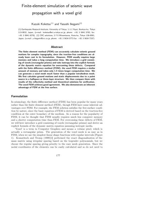
<strong>Finite</strong>-<strong>element</strong> <strong>simulation</strong> <strong>of</strong> <strong>seismic</strong> <strong>wave</strong><br />
<strong>propagation</strong> with a voxel grid<br />
Kazuki Koketsu (1) and Yasushi Ikegami (2)<br />
(1) Earthquake Research Institute, University <strong>of</strong> Tokyo, 1-1-1 Yayoi, Bunkyo-ku, Tokyo<br />
113-0032, Japan, (e-mail: koketsu@eri.u-tokyo.ac.jp, phone: +81 3 5841 5782, fax:<br />
+81 3 5841 8278). (2) CRC solutions, 2-7-5 Minamisuna, Koto-ku, Tokyo 136-8581,<br />
Japan, (e-mail: y-ikegami@crc.co.jp, phone: +81 3 5634 5773 fax: +81 3 5634 7337)<br />
Abstract<br />
The finite <strong>element</strong> method (FEM) can accurately calculate <strong>seismic</strong> ground<br />
motions for complex topography, since the traction-free conditions are already<br />
been cast in its formulation. However, FEM usually requires large<br />
memory and takes a long computation time. We introduce a grid consisting<br />
<strong>of</strong> voxels (rectangular prisms) and take isotropy into the explicit formula<br />
<strong>of</strong> the dynamic matrix equation for overcoming these defects. Compared<br />
with the finite difference method (FDM), the voxel FEM requires a similar<br />
amount <strong>of</strong> memory and takes only 1.4 times longer computation time. We<br />
can generate a voxel mesh much faster than a popular tetrahedron mesh.<br />
We first calculate ground motions and static displacements due to a point<br />
source in a halfspace or three-layer structure. We then compare them with<br />
results <strong>of</strong> the reflectivity method and theoretical solutions for verification.<br />
The voxel FEM achieves good agreement. We also demonstrate an inherent<br />
advantage <strong>of</strong> FEM at the free surface.<br />
Formulation<br />
In seismology, the finite difference method (FDM) has been popular for many years<br />
rather than the finite <strong>element</strong> method (FEM), though FEM have some inherent advantages<br />
over FDM.For example, the FEM solution satisfies the free-surface condition<br />
by nature, since the basic equation <strong>of</strong> FEM is derived based on the traction-free<br />
condition at the outer boundary <strong>of</strong> the medium.As a reason for the popularity <strong>of</strong><br />
FDM, it can be thought that FDM usually requires much less computer memory<br />
and a shorter computation time than FEM.For overcoming these defects <strong>of</strong> FEM,<br />
we will here introduce a grid consisting <strong>of</strong> voxels (rectangular prisms) and derive an<br />
explicit formula <strong>of</strong> the dynamic matrix equation assuming isotropic media.<br />
‘Voxel’ is a term in Computer Graphics and means a volume pixel, which is<br />
actually a rectangular prism.The generation <strong>of</strong> the voxel mesh is as easy as in<br />
FDM, when we use the simplest linear shape functions with regular intervals (Figure<br />
1).Komatitsch and Tromp (1999)[4] performed the exact diagonalization <strong>of</strong> the<br />
mass matrix using irregular spacing based on the Legendre polynomials, but we<br />
choose the regular spacing giving priority to the easy mesh generation.Since the<br />
nodal coordinates <strong>of</strong> the <strong>element</strong>s can be easily calculated and so do not need to<br />
177
e memorized for this regular spacing, memory requirement is significantly reduced<br />
compared to the case where the coordinates are memorized.<br />
Figure 1: Voxels in a medium.<br />
Secondly we take isotropy into the formulation explicitly.If an <strong>element</strong> is fully<br />
anisotropic, there are 24 independent components in the stiffness matrix.However,<br />
according to the symmetry among the isotropic elastic constants and linear shape<br />
functions, the number <strong>of</strong> independent components is reduced to 12.This reduction<br />
is also effective for increasing the computational efficiency <strong>of</strong> FEM.<br />
The voxel FEM has already been implemented for a Beowulf PC cluster with the<br />
MPI library.<br />
Numerical Examples<br />
Figure 2: Ground motions in a halspace (left: reflectivity method, right: FEM).<br />
We calculate ground motions from a point source in the halfspace (V P =4.0<br />
km/s, V S =2.3 km/s, ρ =1.8 g/cm 3 ) or three-layer structure <strong>of</strong> Graves (1996)[2]<br />
using the voxel FEM.We then compare them with results <strong>of</strong> the reflectivity method<br />
(Kohketsu, 1985 [3]) for verification.The voxel FEM achieves good agreement shown<br />
in Figures 2 for three kinds <strong>of</strong> point sources, i.e., a strike slip, 45-degree dip slip and<br />
vertical dip slip at a depth <strong>of</strong> 2.5 km in the halfspace with a cosine time function<br />
1 s long.It takes 1.4 hour for the voxel FEM to complete the 20 s (800 steps;<br />
178
0.025 s interval) time history <strong>of</strong> a 30×30×10 km medium (4,608,000 <strong>element</strong>s; 125 m<br />
interval) on a 1.7 GHz Pentium 4 with 1 GB RIMM memory, while FDM <strong>of</strong> Furumura<br />
et al. (2000)[1] spends 1.0 hours for the same configuration. The voxel FEM requires<br />
a similar amount <strong>of</strong> memory to that <strong>of</strong> FDM.<br />
The next verification is carried out for a strike slip source at a depth <strong>of</strong> 1.6km<br />
in a horizontally layered structure.This three-layer model was also used by Graves<br />
(1996)[2].The FEM code occupies 675MB memory for 12,800,000 <strong>element</strong>s, and<br />
again achieves good agreement as shown in Figure 3.<br />
Figure 3: Ground motions in a layered structure (left: reflectivity method, right: FEM).<br />
Wald and Graves (2001)[6] demonstrated that FDM could calculate even static<br />
displacements if the computation continues for a sufficiently long time.This demonstration<br />
is confirmed using the voxel FEM in the same halfspace for the previous<br />
tests.Figure 4 favorably compares the displacements by FEM with the theoretical<br />
solutions by Okada (1985)[5], though GMT and micro AVS give different impressions<br />
for similar results.<br />
Figure 4: Static displacements due to a strike slip (upper: Okada’s solution, lower: FEM).<br />
One <strong>of</strong> the greatest advantages <strong>of</strong> FEM is that the traction-free condition has<br />
already been cast in the formulation.No special treatment is needed for the free<br />
179
surface.In order to confirm this advantage, another test <strong>of</strong> Graves (1996)[2] is<br />
carried out in the halspace.The dashed FK seismograms in Figure 5 should be<br />
correct.Although the FDM results fail to agree with them, the results by the voxel<br />
FEM achieve good agreement.<br />
Figure 5: Comparison <strong>of</strong> seismograms calculated with the FK technique, FDM using the<br />
modified vacuum formulations, and the voxel FEM.<br />
Acknowledgments<br />
This research was supported by the Japan Science and Technology Corporation under the<br />
ACT-JST program 13C-2.<br />
References<br />
[1] Furumura, T., Wen, K.-L. and Koketsu, K., 2000, PSM/FDM hybrid <strong>simulation</strong><br />
<strong>of</strong> the 1999 Chi-Chi, Taiwan, earthquake, 2nd ACES Workshop, 280–285<br />
[2] Graves, R.W., 1996, Simulating <strong>seismic</strong> <strong>wave</strong> <strong>propagation</strong> in 3D elastic media<br />
using staggered grid finite differences, Bull.Seismol.Soc.Am., 86, 1091–1106<br />
[3] Kohketsu, K., 1985, The extended reflectivity method for synthetic near-field seismograms,<br />
J.Phys.Earth, 33, 121–131<br />
[4] Komatitsch, D.and Tromp, J., 1999, Introduction to the spectral <strong>element</strong> method<br />
for three-dimensional <strong>seismic</strong> <strong>wave</strong> <strong>propagation</strong>, Geophys.J.Int., 139, 806–<br />
822<br />
[5] Okada, Y., 1985, Surface deformation due to shear and tensile faults in a halfspace,<br />
Bull.Seismol.Soc.Am., 75, 1135–1154<br />
[6] Wald, D.J. and Graves, R.W., 2001, Resolution analysis <strong>of</strong> finite fault source<br />
inversion using one- and three-dimensional Green’s functions 2. Combining<br />
<strong>seismic</strong> and geodetic data laws, J.Geophys.Res., 106, 8767–8788<br />
180