Overview of QUIC-SVD - UMass Graphics Lab - University of ...

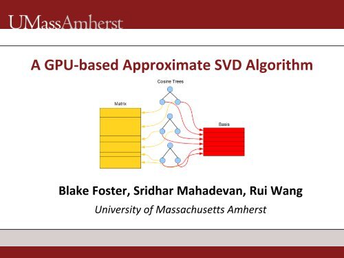
A GPU-based Approximate SVD Algorithm
Blake Foster, Sridhar Mahadevan, Rui Wang
University of Massachusetts Amherst

Introduction
• Singular Value Decomposition (SVD)
• A: m × n matrix (m ≥ n)
• U, V: orthogonal matrices
• Σ: diagonal matrix
• Exact SVD can be computed in O(mn 2 ) time.
2

Introduction
• Approximate SVD
• A: m × n matrix, whose intrinsic dimensionality
is far less than n
• Usually sufficient to compute the k (≪ n) largest
singular values and corresponding vectors.
• Approximate SVD can be solved in O(mnk) time (
compared to O(mn 2 ) for full svd).
3

Introduction
• Sample-based Approximate SVD
• Construct a basis V by directly sampling or taking linear
combinations of rows from A.
• An approximate SVD can be extracted from the projection
of A onto V.
4

Introduction
• Sample-based Approximate SVD
• Construct a basis V by directly sampling or taking linear
combinations of rows from A.
• An approximate SVD can be extracted from the projection
of A onto V.
• Sampling Methods
• Length-squared
[Frieze et al. 2004, Deshpande et al. 2006]
• Random projection
[Friedland et al 2006, Sarlos et al. 2006, Rokhlin et al. 2009]
5

Introduction
• QUIC-SVD [Holmes et al. NIPS 2008]
• Sampled-based approximate SVD.
• Progressively constructs a basis V using a cosine tree.
• Results have controllable L2 error basis construction
adapts to the matrix and the desired error.
6

Our Goal
• Map QUIC-SVD onto the GPU (Graphics Processing Units)
• Powerful data-parallel computation platform.
• High computation density, high memory bandwidth.
• Relatively low-cost.
NVIDIA GTX 580
512 cores
1.6 Tera FLOPs
3 GB memory
200 GB/s bandwidth
$549
7

Related Work
• OpenGL-based: rasterization, framebuffers, shaders
• [Galoppo et al. 2005]
• [Bondhugula et al. 2006]
• CUDA-based:
• Matrix factorizations [Volkov et al. 2008]
• QR decomposition [Kerr et al. 2009]
• SVD [Lahabar et al. 2009]
• Commercial GPU linear algebra package [CULA 2010]
8

Our Work
• A CUDA implementation of QUIC-SVD.
• Up to 6~7 times speedup over an optimized CPU
version.
• A partitioned version that can process large, out-ofcore
matrices on a single GPU
• The largest we tested are 22,000 x 22,000 matrices
(double precision FP).
9

Overview of QUIC-SVD
[Holmes et al. 2008]
A
V
10

Overview of QUIC-SVD
[Holmes et al. 2008]
A
Start from a root node that owns the entire matrix
(all rows).
11

Overview of QUIC-SVD
[Holmes et al. 2008]
A
pivot row →
Select a pivot row by importance sampling the
squared magnitudes of the rows.
12

Overview of QUIC-SVD
[Holmes et al. 2008]
A
pivot row →
Compute inner product of every row with the pivot row.
(this is why it’s called Cosine Tree)
13

Overview of QUIC-SVD
[Holmes et al. 2008]
A
Closer to
zero →
The rest →
Based on the inner products, the rows are partitioned
into 2 subsets, each represented by a child node.
14

Overview of QUIC-SVD
[Holmes et al. 2008]
A
V
Compute the row mean (average) of each subset;
add it to the current basis set (keep orthogonalized).
15

Overview of QUIC-SVD
[Holmes et al. 2008]
A
V
Repeat, until the estimated L2 error is below a threshold.
The basis set now provides a good low-rank approximation.
16

Overview of QUIC-SVD
• Monte Carlo Error Estimation:
• Input: any subset of rows A s , the basis V, δ ∈ [0,1]
• Output: estimated , s.t. with probability at
least 1 − δ, the L2 error:
• Termination Criteria:
17

Overview of QUIC-SVD
• 5 Steps:
1. Select a leaf node with maximum estimated L2 error;
2. Split the node and create two child nodes;
3. Calculate and insert the mean vector of each child to the
basis set V (replacing the parent vector), orthogonalized;
4. Estimate the error of newly added child nodes;
5. Repeat steps 1—4 until the termination criteria is
satisfied.
18

GPU Implementation of QUIC-SVD
• Computation cost mostly on constructing the tree.
• Most expensive steps:
• Computing vector inner products and row means
• Basis orthogonalization
19

Parallelize Vector Inner Products and Row Means
• Compute all inner products and row means in parallel.
• Assume a large matrix, there are sufficient number of
rows to engage all GPU threads.
• An index array is used to point to the physical rows.
20

Parallelize Gram Schmidt Orthogonalization
• Classical Gram Schmidt:
Assume v1 , v2, v3... vn
are in the current basis set (i.e. they
are orthonormal vectors), to add a new vector :
v
( , ) ( , ) ... ( , )
r
1
r where proj( r, v) ( r v)
v
r r proj r v1 proj r v2
proj r v n
n
• This is easy to parallelize (as each projection is independently
calculated), but it has poor numerical stability.
r
21

Parallelize Gram Schmidt Orthogonalization
• Modified Gram Schmidt:
r r proj( r, v ),
1 1
r r proj( r , v ),
2 1 1 2
... ...
r r r proj( r , v )
v r r
n1
k k 1 k 1
k
• This has good numerical stability, but is hard to parallelize, as
the computation is sequential!
22

Parallelize Gram Schmidt Orthogonalization
• Our approach: Blocked Gram Schmidt
(1)
v v proj v u1 proj v u2
proj v um
( , ) ( , ) ... ( , )
v v proj( v , u ) proj( v , u ) ... proj( v , u )
(2) (1) (1) (1) (1)
m1 m2 2m
......
u v proj( v , u ) proj( v , u ) ... proj( v , u )
( n/ m) ( n/ m) ( n/ m) ( n/ m)
k 1 2m1 2m2
k
• This hybrid approach combines the advantages of the
previous two – numerically stable, and GPU-friendly.
23

Extract the Final Result
• Input: matrix A, basis set V
• Output: U, Σ, V, the best approximate SVD of A within
the subspace V.
• Algorithm:
• Compute AV, then (AV) T AV, and SVD
U ′ Σ ′ V′ T = (AV) T AV
• Let V = VV′, Σ = (Σ′) 1/2 , U = (AV)V′Σ −1 ,
• Return U, Σ, V.
24

Extract the Final Result
• Input: matrix A, subspace basis V
• Output: U, Σ, V, the best approximate SVD of A within
the subspace V.
• Algorithm:
• Compute AV, then (AV) T AV, and SVD
U ′ Σ ′ V′ T = (AV) T AV
• Let V = VV′, Σ = (Σ′) 1/2 , U = (AV)V′Σ −1 ,
• Return U, Σ, V.
SVD of a k × k matrix.
25

Partitioned QUIC-SVD
• The advantage of the GPU is only obvious for largescale
problems, e.g. matrices larger than 10,000 2 .
• For dense matrices, this will soon become an out-ofcore
problem.
• We modified our algorithm to use a matrix partitioning
scheme, so that each partition can fit in GPU memory.
26

… …
… …
Partitioned QUIC-SVD
• Partition the matrix into fixed-size blocks
A 1
A 2
A s
27

… …
… …
Partitioned QUIC-SVD
• Partition the matrix into fixed-size blocks
A 1
A 2
A s
28

Partitioned QUIC-SVD
29

Partitioned QUIC-SVD
• Termination Criteria is guaranteed:
30

Implementation Details
• Main implementation done in CUDA.
• Use CULA library to extract the final SVD (this involves
processing a k × k matrix, where k ≪ n).
• Selection of the splitting node is done using a priority
queue, maintained on the CPU side.
• Source code will be made available on our site
http://graphics.cs.umass.edu
31

Performance
• Test environment:
• CPU: Intel Core i7 2.66 GHz (8 HTs), 6 GB memory
• GPU: NVIDIA GTX 480 GPU
• Test data:
• Given a rank k and matrix size n, we generate a n × k left
matrix and k × n right matrix, both filled with random
numbers; the product of the two gives the test matrix.
• Result accuracy:
• Both CPU and GPU versions use double floats; termination
error ε = 10 −12 , Monte Carlo estimation δ = 10 −12 .
32

Performance
• Comparisons:
1. Matlab’s svds;
2. CPU-based QUIC-SVD (optimized, multi-threaded,
implemented using Intel Math Kernel Library);
3. GPU-based QUIC-SVD.
4. Tygert SVD (approximate SVD algorithm, implemented in
Matlab, based on random projection);
33

Performance – Running Time
34

Performance – Speedup Factors
35

Performance – Speedup Factors
36

Performance – CPU vs. GPU QUIC-SVD
Running Time
Speedup
37

Performance – GPU QUIC-SVD vs. Tygert SVD
Running Time
Speedup
38

Integration with Manifold Alignment Framework
39

Conclusion
• A fast GPU-based implementation of an approximate
SVD algorithm.
• Reasonable (up to 6~7 ×) speedup over an optimized
CPU implementation, and Tygert SVD.
• Our partitioned version allows processing out-of-core
matrices.
40

Future Work
• Be able to process sparse matrices.
• Application in solving large graph Laplacians.
• Components from this project can become building
blocks for other algorithms: random projection trees,
diffusion wavelets etc.
41

Acknowledgement
• Alexander Gray
• PPAM reviewers
• NSF Grant FODAVA-1025120
42