A Mathematical Model of Refinery Operations Characterised by ...
A Mathematical Model of Refinery Operations Characterised by ...
A Mathematical Model of Refinery Operations Characterised by ...

You also want an ePaper? Increase the reach of your titles
YUMPU automatically turns print PDFs into web optimized ePapers that Google loves.
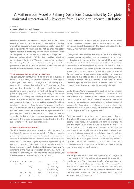
A <strong>Mathematical</strong> <strong>Model</strong> <strong>of</strong> <strong>Refinery</strong> <strong>Operations</strong> <strong>Characterised</strong> <strong>by</strong> Complete<br />
Horizontal Integration <strong>of</strong> Subsystems from Purchase to Product Distribution<br />
Logistics<br />
a report <strong>by</strong><br />
Adebayo Alabi and Jordi Castro<br />
Department <strong>of</strong> Statistics and <strong>Operations</strong> Research, Universitat Politecnica de Catalunya, Barcelona<br />
<strong>Refinery</strong> economics are extremely complex and involve massive<br />
amounts <strong>of</strong> operational data and decision-making processes; therefore,<br />
most refinery planners model and solve each sub-problem sequentially<br />
and independently. Obviously, this does not guarantee the globally<br />
optimal operation <strong>of</strong> the refinery because several features in a single<br />
and integrated model are not considered. Each sub-problem <strong>of</strong><br />
integrated refinery planning (IRP) has been modelled, solved and<br />
well-published in the literature. 1 Currently, research efforts are directed<br />
towards integrating the sub-problems and solving the resulting<br />
problem. 2,3 In this article, the IRP problem is introduced and the<br />
solution methods with results are then outlined.<br />
The Integrated <strong>Refinery</strong> Planning Problem<br />
The general system configuration <strong>of</strong> the IRP problem is illustrated in<br />
Figure 1. In this article, the problem statement is summarised as<br />
follows: given 10 oil tankers, 10 storage tanks, five blending tanks, a<br />
network <strong>of</strong> four refineries, five final products, 60 depots and all <strong>of</strong> the<br />
necessary data, determine the cash flow, material flow and tank<br />
inventories in order to minimise the total cost during the planning<br />
period ranging from two to 300 days while satisfying the process<br />
constraints. The supply and blending models are taken from<br />
references 4 and 5, respectively. Generally, material balance around<br />
each process unit, flow <strong>of</strong> materials and inventory pr<strong>of</strong>iles with the<br />
associated costs are outlined in each sub-problem, distribution<br />
inclusive. In addition, use <strong>of</strong> the processing units must not exceed<br />
specified capacity while meeting demand for a given material at a<br />
given destination. Material balances around process units that are<br />
situated at the border <strong>of</strong> two given sub-systems generate linking<br />
constraints. The objective is to minimise the total costs <strong>of</strong> the three<br />
sub-problems over the entire planning horizon.<br />
Solution Methods and Results<br />
The IRP problem was implemented in AMPL modelling language. From<br />
the plot <strong>of</strong> the constraint matrix generated in AMPL, each planning<br />
period displayed a primal block-angular structure, as reported in<br />
reference 1. The IRP problem can, therefore, be algebraically expressed<br />
as in Equation 1. Matrices B 1 , B 2 and B 3 represent supply, blending and<br />
distribution constraints, respectively, while A 1 , A 2 and A 3 represent<br />
linking constraints <strong>of</strong> supply, blending and distribution respectively. The<br />
dimensions <strong>of</strong> the resulting optimisation problems (i.e. number <strong>of</strong><br />
variables and constraints, and non-zeros <strong>of</strong> the constraints matrix) for<br />
the seven instances considered are reported in Table 1.<br />
z* = min. c 1 x 1 + c 2 x 2 + c 3 x 3 = z (1)<br />
s.t B 1 x 1 (≤, = or ≥) b 1<br />
B 2 x 2 (≤, = or ≥) b 2<br />
B 3 x 3 (≤, = or ≥) b 3<br />
A 1 x 1 + A 2 x 2 + A 3 x 3 (≤, = or ≥) b 3<br />
x 1 , x 2 , x 3 ≥ 0<br />
Primal block-angular problems such as Equation 1 can be solved<br />
<strong>by</strong> decomposition techniques such as Dantzig–Wolfe and block<br />
co-ordinate–descent decomposition. This choice was justified <strong>by</strong> the<br />
relatively small number <strong>of</strong> linking constraints. 1<br />
Dantzig–Wolfe decomposition relies on the fact that a non-empty,<br />
bounded convex polyhedron can be represented as a convex<br />
combination <strong>of</strong> its extreme points – the original IRP problem was<br />
therefore re-formulated into a master problem and three sub-problems.<br />
Each variable in the master problem represents a solution to one <strong>of</strong> the<br />
three sub-problems. The master problem then requests additional<br />
solutions from the sub-problem such that the total cost is reduced<br />
further. 6 Block co-ordinate–descent decomposition minimises the<br />
total cost with respect to variables in a given sub-problem, while the<br />
variables in the remaining sub-problems are kept constant. This is<br />
iteratively repeated until the difference between subsequent and<br />
current total cost is less than a specified optimality tolerance.<br />
Unlike Dantzig–Wolfe decomposition, block co-ordinate–descent<br />
decomposition does not always converge to an optimum, but<br />
convergence is guaranteed if the problem is strictly convex<br />
(which is not the case in the IRP problem). Some recent specialised<br />
interior-point decomposition approaches have not been considered<br />
because they have either been shown to be more efficient for<br />
problems with many (even non-linear) sub-problems 7 or rely on some<br />
specific properties <strong>of</strong> the linking constraints. 8<br />
Both decomposition techniques were implemented in Matlab.<br />
The whole IRP problem, as well as each sub-problem within the<br />
decomposition framework, was solved with both the interior-point<br />
and dual simplex CPLEX options. Results are reported in Table 2. The<br />
results suggest that: interior-point methods could solve all<br />
the instances but would require a large computational time;<br />
interior-point-based decomposition techniques outperformed the<br />
dual-simplex-based techniques; decomposition techniques were<br />
competitive to obtain a good feasible solution, and they solved to<br />
optimality all <strong>of</strong> the instances until 120 days; and block<br />
co-ordinate–descent seems the most effective approach if one is<br />
looking for a good and quick solution.<br />
Conclusions<br />
The IRP problem was modelled and implemented as a large-scale<br />
linear programming (LP) problem characterised <strong>by</strong> primal block<br />
angular structure. The problem was therefore effectively solved <strong>by</strong><br />
Dantzig–Wolfe and block co-ordinate–descent decomposition<br />
techniques, the latter resulting in the most effective approach. Work<br />
is in progress to study the use <strong>of</strong> alternative interior-point-based<br />
decomposition techniques 7,8 and incorporate binary decision<br />
variables into the IRP model. n<br />
© T O U C H B R I E F I N G S 2 0 0 9<br />
55
A <strong>Mathematical</strong> <strong>Model</strong> <strong>of</strong> <strong>Refinery</strong> <strong>Operations</strong><br />
Figure 1: Graphical Overview <strong>of</strong> the Integrated Sub-systems<br />
Supply sub-system Refining sub-system Distribution sub-system<br />
V<br />
Oil tankers<br />
I<br />
Storage tanks<br />
J<br />
Blending tanks<br />
L<br />
Refineries<br />
PT<br />
Product tanks<br />
DP<br />
Depots<br />
Table 1: Dimensions <strong>of</strong> the Integrated <strong>Refinery</strong> Planning Problem for Planning Period <strong>of</strong> Two to 300 Days<br />
Period (days) Without CPLEX Pre-solve Option With CPLEX Pre-solve Option<br />
Constraints Variables Non-zeros Constraints Variables Non-zeros<br />
2 7,211 13,697 45,389 3,012 5,798 24,996<br />
3 10,883 20,540 70,049 4,838 9,022 40,374<br />
60 220,187 410,591 3,409,679 97,520 181,390 2,809,890<br />
120 440,507 821,171 11,031,779 195,080 362,830 9,831,870<br />
180 660,827 1,231,751 22,865,879 281,840 533,470 21,044,250<br />
240 881,147 1,642,331 38,911,979 375,800 711,310 36,483,030<br />
300 1,101,467 2,052,911 59,170,079 469,760 889,150 56,133,810<br />
Table 2: Summary Solution for the Integrated <strong>Refinery</strong> Planning Problem Suite<br />
Planning Period (days) Whole IRP Problem IRP Decomposition<br />
Block Co-ordinate–Descent<br />
Dantzig–Wolfe<br />
Dual Simplex Interior Point Dual Simplex Interior Point Dual Simplex Interior Point<br />
CPU (seconds) CPU (seconds) CPU (seconds) CPU (seconds) CPU (seconds) CPU (seconds)<br />
Iterations Cost (US$) Iterations Cost (US$) Iterations Cost (US$) Iterations Cost (US$) Iterations Cost (US$) Iterations Cost (US$)<br />
2 0.4 0.5 1.2 0.8 7.5 5.4<br />
4,933 28 3 2 7 5<br />
146,320.4 146,320.4 147,713.6 147,713.6 147,713.6 147,713.6<br />
3 1.8 0.9 3.8 1.3 9.7 8.2<br />
9,070 26 12 10 170 91<br />
290,699.5 290,699.5 290,699.5 290,699.5 290,699.5 290,699.5<br />
60 2,834.8 1,798.8 3,569.5 1,787.9 5,758.9 3,183.9<br />
38,3629 28 15 12 182 154<br />
4,232,012.8 4,232,012.8 4,232,012.8 4,232,012.8 4,232,012.8 4,232,012.8<br />
120 37,337.5 14,689.9 22,903.6 14,596.4 25,783.0 22,440.7<br />
844,162 30 22 18 194 169<br />
8,655,432.5 8,655,432.5 11,827,901.2 11,827,901.2 11,827,901.2 11,827,901.2<br />
180 235,214.0 37,432.1 26,487.8 18701.2 31,783.6 28,966.2<br />
138,8429 29 28 20 205 182<br />
12,625,528.7 12,625,528.7 17,922,205.4 17,922,205.4 17,922,205.4 17,922,205.4<br />
240 >878,081.3 † 99,907.6 32,543.1 23,194.8 33,981.6 29,255.9<br />
>1,081,000 † 31 30 27 209 193<br />
16,731,729.3 16,731,729.3 36,004,503.1 36,004,503.1 36,004,503.1 36,004,503.1<br />
300 >842,000.3* 215,531.9 34,009.5 26,369.5 39,128.9 31,014.6<br />
> 540,000* 35 35 32 219 205<br />
20,888,039.6 20,888,039.6 48,282,344.0 48,282,344.0 48,282,344.0 48,282,344.0<br />
† Stopped very far from optimality, with an objective value <strong>of</strong> 3887976.3. *Stopped very far from optimality, with an objective value <strong>of</strong> -4596190.7.<br />
1. Alabi A, Castro J, Comput Oper Res, 2009;36:2472–83<br />
2. Lasschuit W, Thijssen N, Supporting supply chain planning<br />
and scheduling decisions in the oil and chemical industry. In:<br />
Grossmann IE, McDonald CM (eds), Proceedings <strong>of</strong> fourth<br />
international conference on foundations <strong>of</strong> computer-aided<br />
process operations, Coral Springs: CAChE, 2003;37–44.<br />
3. Moro LFL, , Comp Chemical Eng, 2003;27:1303–5.<br />
4. Song J, Park H, Lee D-Y, Park S, Ind Eng Chem Res,<br />
41;2002:4794–806.<br />
5. Aron<strong>of</strong>sky JS, Dutton JM, Tayyabkhan MT, Managerial Planning<br />
With Linear Programming: In Process Industry <strong>Operations</strong>, John Wiley and<br />
Sons, Inc., 1978.<br />
6. Tebboth JR, A Computational Study <strong>of</strong> Dantzig–Wolfe Decomposition,<br />
PhD Thesis, University <strong>of</strong> Buckingham, 2001.<br />
7. Conejo AJ, Nogales FJ, Prieto FJ, <strong>Mathematical</strong> Programming,<br />
2002;93:495–515.<br />
8. Castro J, An interior-point approach for primal block-angular<br />
problems, Computational Optimization and Applications,<br />
2007;36:195–219.<br />
56<br />
H Y D R O C A R B O N W O R L D V O L U M E 4 I S S U E 2