Soil & GW Remediation â From Site Assessment to Final Closure (I)
Soil & GW Remediation â From Site Assessment to Final Closure (I)
Soil & GW Remediation â From Site Assessment to Final Closure (I)

You also want an ePaper? Increase the reach of your titles
YUMPU automatically turns print PDFs into web optimized ePapers that Google loves.
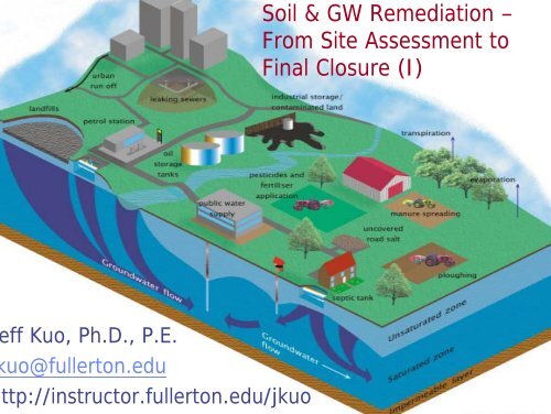
<strong>Soil</strong> & <strong>GW</strong> <strong>Remediation</strong> –<br />
<strong>From</strong> <strong>Site</strong> <strong>Assessment</strong> <strong>to</strong><br />
<strong>Final</strong> <strong>Closure</strong> (I)<br />
ff Kuo, Ph.D., P.E.<br />
uo@fuller<strong>to</strong>n.edu<br />
ttp://instruc<strong>to</strong>r.fuller<strong>to</strong>n.edu/jkuo<br />
1
Content<br />
UST removal procedure<br />
Remedial investigation<br />
Groundwater and soil sampling<br />
Characterization of vadoze zone<br />
Characterization of groundwater<br />
movement<br />
Mass partition in different phases<br />
Fate & transport of contaminants<br />
Aquifer res<strong>to</strong>ration<br />
2
3<br />
Content…<br />
<strong>Soil</strong> remediation<br />
technologies<br />
<strong>GW</strong> remediation<br />
technologies<br />
Treatment of VOC-laden<br />
air<br />
Selection of remedial<br />
technologies<br />
<strong>Final</strong> closure<br />
Modeling
UST Removal Procedure<br />
His<strong>to</strong>rical record<br />
Pre-drilling<br />
Permitting<br />
• Fire department<br />
• Local environmental agency<br />
• Air quality management districts<br />
Dig-alert<br />
Sampling locations<br />
• EPA methods (EPA 8015, EPA 8020, EPA 418.1,….)<br />
• Certified labs<br />
Additional excavation<br />
Separation of contaminated soils<br />
4
Remedial<br />
Investigation<br />
What chemicals are present?<br />
Where, on the site, are these chemicals located?<br />
His<strong>to</strong>rical records<br />
• What industrial activities occurred at the <strong>Site</strong>?<br />
• What chemicals were used at the <strong>Site</strong>?<br />
• Where were they used?<br />
• Were chemicals s<strong>to</strong>red in tanks? Where? Are<br />
they still in the tanks?<br />
How much of these chemicals were released?<br />
• Records?<br />
• Recollection of employees?<br />
5
Common Remedial<br />
Investigation (RI)<br />
Activities<br />
Removal of contamination source(s) such as<br />
leaky USTs<br />
Installation of soil borings (Boring?)<br />
Installation of groundwater moni<strong>to</strong>ring wells<br />
<strong>Soil</strong> sample collection and analysis<br />
Groundwater sample collection and analysis<br />
Aquifer testing<br />
6
Data Collected from RI<br />
Types of contaminants present in soil and gw<br />
Concentrations of contaminants in the collected<br />
samples<br />
Vertical and areal extents of contaminant plumes in<br />
soil and gw<br />
Vertical and areal extents of free-floating product or<br />
the DNAPLs<br />
<strong>Soil</strong> characteristics including the types of soil,<br />
density, moisture content, etc.<br />
Groundwater elevations<br />
Drawdown data collected from aquifer tests<br />
7
Groundwater and <strong>Soil</strong> Sampling<br />
8
<strong>Soil</strong> Gas Survey<br />
9
<strong>Soil</strong> Gas Survey<br />
Good remote sensing <strong>to</strong>ol for locating VOCs<br />
Also used <strong>to</strong> defined gw plume.<br />
For sandy formation, it may over-estimate the<br />
problem.<br />
Inexpensive and fast.<br />
10
General Considerations<br />
Types of Moni<strong>to</strong>ring<br />
Sampling Pro<strong>to</strong>col<br />
Types of Samples<br />
Sampling Location<br />
Sampling Frequency<br />
Sampling Size, Bottles, Preservation<br />
11
Types of Moni<strong>to</strong>ring/Sampling<br />
Detection Moni<strong>to</strong>ring<br />
• presence of contamination condition<br />
• existing drinking water wells?<br />
<strong>Assessment</strong> Moni<strong>to</strong>ring<br />
• extent and magnitude of contamination<br />
Evaluation Moni<strong>to</strong>ring<br />
• data for remediation system design<br />
Performance Moni<strong>to</strong>ring<br />
• evaluation of remediation effort<br />
12
Sampling Pro<strong>to</strong>col<br />
Objectives<br />
• Property transfer<br />
• Environmental liability (establish baseline for<br />
insurance/mortgage, clean-up)<br />
Locations, frequencies, types, methods, H&S<br />
Information needed for design a sampling plan<br />
• site his<strong>to</strong>ry (spill, operation, disposal practices)<br />
• site geology and hydrogeology<br />
Good documentation (always)<br />
Leave room for evolutionary development<br />
• collect more, analyze less<br />
13
Types of Samples<br />
QA/QC are important concerns!<br />
Field Blank (p. 90 EPA manual)<br />
• DI water from lab → field → sample vial→ lab<br />
• Used <strong>to</strong> determine the limit of detection<br />
Rinse/Cleaning Blank<br />
• contaminated from previous sample?<br />
Duplicate Samples<br />
• collected as back-up<br />
• soil samples are commonly duplicated.<br />
Replicate Samples<br />
• sub-samples of the same sample<br />
• labeled separately <strong>to</strong> estimate lab precision<br />
14
Types of Samples<br />
Split Samples<br />
QA/QC are important concerns!<br />
• split in half in the field <strong>to</strong> two labs or<br />
regula<strong>to</strong>ry agency<br />
Spiked Samples<br />
• spiked w/a reference standard in the lab<br />
• estimate recovery and matrix interference<br />
Labora<strong>to</strong>ry Blank<br />
• DI water analyzed <strong>to</strong> determine lab<br />
contamination<br />
Standard Reference Samples<br />
• detect instrument calibration error or analytical<br />
15
16<br />
Types of Samples ….<br />
Travel Blank<br />
Grab Sample vs. Composite Sample<br />
• cost saving?<br />
• field or lab? depth or area?<br />
• time-weighted or volume/mass-weighted?<br />
• be careful about VOCs<br />
QA/QC are important concerns
Locations & Number<br />
of Samples<br />
Statistically based sampling plans<br />
• Number of samples determined statistically.<br />
• Location of samples determined by selecting<br />
n sample points from m potential points at<br />
random.<br />
Judgmentally based sampling plans<br />
• need some knowledge (soil gas survey,<br />
surface geophysical technique, Hydropunch)<br />
17
Locations & Number<br />
of Samples…<br />
Use US EPA’s Data Quality Objective Process<br />
• Used by USEPA <strong>to</strong> ensure consistent national<br />
approach <strong>to</strong> environmental sampling.<br />
• Systematic, rational approach <strong>to</strong> determine<br />
when, where, and how <strong>to</strong> collect samples or<br />
measurements.<br />
18
Locations & Number of Samples ...<br />
Kuo’s suggestions/approach<br />
Start from the center of source (if known)<br />
Go outward for a specific distance<br />
Another distance, if contaminated<br />
Cut back half-way, if not contaminated<br />
Vadose zone: every 5 <strong>to</strong> 10 ft<br />
At the property line?<br />
19
Sampling Frequency<br />
Quarterly (most of time is OK) for <strong>GW</strong> sampling<br />
• survey all wells quarterly, part of them<br />
monthly<br />
Intermittent or slug source<br />
• need more frequent sampling<br />
20
Sampling Size, Containers, and<br />
Preservation Method<br />
Large enough <strong>to</strong> be representative & for analysis<br />
Bottles (EPA Table 9-14, p. 147)<br />
• plastics (Teflon?)<br />
• glass (transparent or amber)<br />
• head-space free (40-ml VOA vial)<br />
• metal<br />
Preservation Method<br />
Chain of Cus<strong>to</strong>dy<br />
Holding Time<br />
On-site Measurement<br />
21
23<br />
adose Zone Sampling –<br />
nalyte selection<br />
Target Compounds<br />
Subsurface<br />
Chemistry<br />
• CEC<br />
Microbial<br />
Geology<br />
• grain size<br />
distribution<br />
• porosity, K
Vadose Zone Sampling –<br />
Surface sampling<br />
Hand Sampling (surface) –<br />
scoops<br />
Hand Sampling (subsurface)<br />
• Hand Augers<br />
• Limited sample depth<br />
Direct Push Samplers<br />
• <strong>From</strong> greater depths<br />
• Allow stratified sampling.<br />
• Hydraulic hammer<br />
24
Vadose Zone Sampling –<br />
On-site analysis<br />
25<br />
No direct reading instruments yet for contaminants<br />
at needed low level detection limits.<br />
On-site methods may be used in some cases.<br />
Few methods approved by USEPA.<br />
Limited <strong>to</strong> specific contaminants.<br />
On-site mobile lab.<br />
Use PID (pho<strong>to</strong>-ionization detec<strong>to</strong>r), FID (flameionization<br />
detec<strong>to</strong>r), OVA (organic vapor analyzer),<br />
LEL (lower explosive limit) for screening.
26<br />
adose Zone Sampling –<br />
rilling<br />
Auger<br />
• Minimal damages <strong>to</strong> aquifer<br />
• No drilling fluid required<br />
• Flight acts as temporary<br />
casing<br />
• Good for unconsolidated<br />
deposits<br />
• Limited <strong>to</strong> 150 ft in depth<br />
Rotary<br />
Cable Tool
Vadose Zone Sampling –<br />
Standard penetration test<br />
A 2" dia, 18" length split core sampler is used in the<br />
Standard Penetration Test (ASTM-D-1586-84), <strong>to</strong><br />
measure soil resistance <strong>to</strong> core penetration.<br />
This test consists of driving the core sampler in<strong>to</strong><br />
the soil by dropping a 140-lb hammer 30” in<br />
repetitive blows. Using an 18" sampler, the number<br />
of blows for three successive 6" penetration<br />
increments are counted.<br />
The number of blows corresponding <strong>to</strong> the first 6"<br />
increment is discarded, while the blows for the<br />
remaining two increments are combined and<br />
reported as the number of blows per foot. 27
Standard penetration test<br />
28
29<br />
Amount of Cuttings from <strong>Soil</strong> Boring<br />
1: Determine the diameter of the boring, d b.<br />
2: Determine the depth of the boring, h.<br />
3: Calculate the volume of the cutting using the<br />
following formula:<br />
Volume of cuttings<br />
π 2<br />
= ∑ ( db<br />
)( h)( fluffy fac<strong>to</strong>r)<br />
4
Groundwater Moni<strong>to</strong>ring - Objectives<br />
Groundwater level<br />
Groundwater quality<br />
• Target Compounds<br />
• DO, pH, conductance<br />
• Dissolved gas<br />
• Fe, Mn, carbonates<br />
• If TCE, then DCE, vinyl chloride<br />
Presence of free-floating product<br />
Aquifer testing<br />
Extraction of groundwater<br />
30
Groundwater<br />
Wells - Design<br />
31<br />
Location<br />
No. of wells<br />
Diameter, Depth<br />
Perforation<br />
• interval, size, method<br />
Packing materials<br />
Permit<br />
Drilling method<br />
H & S
Groundwater Wells -<br />
Construction Materials<br />
Main Considerations<br />
• Compatibility<br />
• Cost<br />
• Handling<br />
• Strength<br />
Choices (EPA Table 4-3, p. 44)<br />
• PVC, PTFE, PP, PE<br />
• Steel, SS<br />
Flexible Joints<br />
32
Groundwater Wells - Sampling<br />
Wells need <strong>to</strong> be developed after installation<br />
Well inspection<br />
Purging<br />
• Remove stagnant water<br />
• 3-5 pore volumes (well casing + filter pack)<br />
• May want <strong>to</strong> minimize purge water<br />
• Moni<strong>to</strong>r pH, conductivity, and temperature - until<br />
stabilized.<br />
• EPA Figure 9-9 and Table 9-8.<br />
Sample collection<br />
Field blanks/rinse blanks<br />
S<strong>to</strong>rage and transport<br />
33
34<br />
<strong>GW</strong> Sampling - Containers<br />
Head space free<br />
Minimize aeration and air contact<br />
Dedicated for each well<br />
No or little adsorption<br />
Teflon, PP, PE: good<br />
PVC, Tygon, silicon rubber - NG
<strong>GW</strong> Sampling - Devices<br />
Bailers<br />
• art, in-line measurement of<br />
pH …. is impossible<br />
• Not good for purging<br />
(homogenize well volume<br />
only)<br />
Bladder Pumps<br />
• cylinder w/ an internal bladder<br />
that compress and expanded<br />
by a gas.<br />
• precise and pulseless flow.<br />
Submersible Pumps<br />
• deep well with high volume,<br />
poor accuracy<br />
35
<strong>GW</strong> Sampling - Hydropunch<br />
The Hydropunch is pushed <strong>to</strong> the<br />
desired depth and the push pipes<br />
are retracted, exposing the<br />
Hydropunch screen <strong>to</strong> the<br />
groundwater.<br />
The groundwater enters and is<br />
allowed <strong>to</strong> come <strong>to</strong> equilibrium,<br />
which generally takes less than 15<br />
<strong>to</strong> 20 minutes.<br />
One-time deal – no permanent well<br />
installation.<br />
36
Well Volumes for<br />
Groundwater<br />
Sampling<br />
Well volume = volume of the groundwater<br />
enclosed inside the well casing + volume of the<br />
groundwater in the pore space of the packing.<br />
π 2 π 2 2<br />
Well volume = [ dc ] h+ [ ( d −d ) h]<br />
φ<br />
4 4<br />
b c<br />
37
38<br />
Well Volumes for <strong>GW</strong><br />
Sampling - Example<br />
The water depth inside one of the four<br />
moni<strong>to</strong>ring wells was measured <strong>to</strong> be 14.5’.<br />
Three well volumes need <strong>to</strong> be purged out<br />
before sampling. Calculate the amount of<br />
purge water and also the number of 55-gallon<br />
drums needed <strong>to</strong> s<strong>to</strong>re the water. Assume<br />
the porosity of the well packing <strong>to</strong> be 0.40.
Well Volumes for <strong>GW</strong> Sampling - Example<br />
π 2 π 2 2<br />
Well volume = [ dc ] h+ [ ( d −d ) h]<br />
φ<br />
4 4<br />
b c<br />
) Well volume = (π/4)(4/12) 2<br />
(14.5) + (π/4)[(10/12) 2 -<br />
(4/12) 2 ](14.5)(0.4) = 13.92 ft 3<br />
) 3 well volumes =<br />
(3)(13.92)=41.8 ft 3 = 313<br />
gallons<br />
) Number of 55-gallon drums<br />
needed= (41.8 ft 3 )(7.48<br />
gal/ft 3 ) ÷ (55 gallon/drum) =<br />
5.7 drums<br />
39
Chemical Compounds of Concern<br />
40
41<br />
Chemical Compounds of Concern<br />
Common examples of chlorinated solvents
Chemical Compounds of Concern<br />
42<br />
Common examples of aromatics<br />
trachlorodibenzo-p-dioxin
43<br />
Chemical Compounds of Concern<br />
Others
Vadose Zone ….<br />
Contaminants may be present in<br />
• Vadose zone<br />
• vapors in the void<br />
• free product in the void<br />
• dissolved in soil moisture<br />
• adsorbed on<strong>to</strong> the soil matrix<br />
• floating on <strong>to</strong>p of the capillary fringe (for LNAPLs)<br />
• Groundwater<br />
• dissolved in the groundwater<br />
• adsorbed on<strong>to</strong> the aquifer material<br />
• sitting on <strong>to</strong>p of the bedrock (for DNAPLs)<br />
44
Mass & volume of soil excavated<br />
during tank removal<br />
Mass & volume of contaminated soil<br />
left in thevadosezone<br />
Mass of contaminants in the vadose<br />
zone<br />
Mass & volume of the free-floating<br />
product<br />
Volume of contaminated groundwater<br />
Mass of contaminants in the aquifer<br />
<strong>GW</strong> flow gradient and direction<br />
Hydraulic conductivity of the aquifer<br />
45<br />
Common Engineering<br />
Calculation Related <strong>to</strong> RI
Mass-concentration<br />
Relationship (ppm)<br />
Liquid: 1 ppm = 1/1,000,000 ~ 1 mg/L<br />
1% by wt. = 10,000 ppm<br />
Solid: 1 ppm = 1 mg/kg =1,000 ppb<br />
Air: ppmV<br />
1ppmV =<br />
MW 224 .<br />
[ mg/ m ] at 0 C<br />
MW<br />
=<br />
2405 . mg m<br />
3<br />
[ / ] at<br />
o<br />
20 C<br />
MW<br />
=<br />
245 . mg m<br />
3<br />
[ / ] at<br />
o<br />
25 C<br />
3<br />
o<br />
6<br />
1ppmV −<br />
= × 10<br />
359<br />
3<br />
[ lb/ ft ]<br />
o<br />
at 32 F<br />
MW<br />
−6 = × 10<br />
385<br />
3<br />
[ lb/ ft ]<br />
o<br />
at 68 F<br />
MW<br />
−6 = × 10<br />
392<br />
3<br />
[ lb/ ft ]<br />
o<br />
at 77 F<br />
46
47<br />
Mass-concentration<br />
Relationship ….<br />
Mass of contaminant in liquid =<br />
(liquid volume)(liquid concentration)<br />
= (V l<br />
)(C)<br />
Mass of contaminant in soil = (X)(M s<br />
)<br />
= (X)[(V s<br />
)(ρ b<br />
)]<br />
Mass of contaminant in air =<br />
(air volume)(concentration in mass/vol)<br />
= (V a<br />
)(G)
Mass-concentration Relationship (Example)<br />
Which of the following media contains the largest<br />
amount of xylene (show your calculations)?<br />
(a) 1 million gallons of water containing 10 ppm of<br />
xylene<br />
(b) 100 cubic yards of soil (bulk density = 1.8<br />
g/cm 3 ) with 10 ppm of xylene<br />
(c) An empty warehouse (200' x 50' x 20') with 10<br />
ppmV xylene in air.<br />
48
Mass-concentration Relationship (Example)<br />
(a) Mass of contaminant in liquid = (V)(C)<br />
= (1,000,000 gallon)(3.785 L/gallon)(10 mg/L) = 3.79 x 10 7 mg<br />
(b) Mass of contaminant in soil = (X)[(V s )(ρ b )]<br />
= [(100 yd 3 )(27 ft 3 /yd 3 )(30.48cm/ft) 3 ][(1.8g/cm 3 )(kg/1000g)](10<br />
mg/kg) = 1.37 x 10 6 mg<br />
(c) Molecular weight of xylene [C 6 H 4 (CH 3 ) 2 ] = 106 g/mole<br />
10 ppmV = (10)(MW of xylene/24.05) mg/m 3 = (10)(106/24.05)<br />
mg/m 3 = 44.07 mg/m 3<br />
Mass of contaminant in air = (V)(G)<br />
= [(200 x 50 x 20 ft 3 )(0.3048m/ft) 3 ](44.07 mg/m 3 ) = 2.5x10 5 mg<br />
49
ass & Volume of <strong>Soil</strong><br />
om a Tank Pit<br />
xample)<br />
Step 1: Measure the dimensions of the<br />
tank pit.<br />
Step 2: Calculate the volume of the tank<br />
pit from the measured dimensions.<br />
Step 3: Determine the number and<br />
volumes of the USTs removed.<br />
Step 4: Subtract the <strong>to</strong>tal volume of the<br />
USTs from volume of the tank pit.<br />
Step 5: Multiply the value from Step #4<br />
50
Mass & Volume of<br />
<strong>Soil</strong> from a Tank Pit<br />
(Example)<br />
(Example) Two 5,000-gallon USTs and one<br />
4,000-gallon UST were removed. The<br />
excavation resulted in a tank pit of 50’ x 24’ x<br />
18’. The excavated soil was s<strong>to</strong>ckpiled on-site.<br />
The bulk density of soil in-situ (before<br />
excavation) = 1.8 g/cm 3 and bulk density of soil<br />
in the s<strong>to</strong>ckpiles is 1.64 g/cm 3 .<br />
Estimate the mass and volume of the excavated<br />
soil.<br />
51
Mass & Volume of <strong>Soil</strong> from<br />
a Tank Pit (Example)<br />
Volume of the tank pit = (50’)(24’)(18’) = 21,600 ft 3 .<br />
Total volume of the USTs = (2)(5,000) + (1)(4,000)<br />
= 14,000 gallons<br />
= (14,000 gallon)(ft 3 /7.48 gallon) = 1,872 ft 3 .<br />
Volume of soil in the tank pit before removal =<br />
(volume of tank pit) - (volume of USTs)<br />
= 21,600 - 1,872 = 18,728 ft 3 .<br />
Volume of soil excavated (in the s<strong>to</strong>ckpile)<br />
= (volume of soil in the tank pit) x (fluffy fac<strong>to</strong>r)<br />
= (18,728)(1.10) = 20,600 ft 3<br />
= (20,600 ft 3 )[yd 3 /27 ft 3 ]= 763 yd 3 .<br />
52
Mass & Volume of <strong>Soil</strong><br />
from a Tank Pit<br />
(Example)<br />
Mass of soil excavated = (volume of the soil in the<br />
tank pit)(bulk density of soil in-situ)<br />
= (volume of the soil in the s<strong>to</strong>ckpile)(bulk density<br />
of soil in the s<strong>to</strong>ckpile)<br />
<strong>Soil</strong> density in situ =<br />
(1.8 g/cm 3 )[(62.4lb/ft 3 )/(1g/cm 3 )]= 112 lb/ft 3 .<br />
<strong>Soil</strong> density in s<strong>to</strong>ckpiles =<br />
(1.64)(62.4) = 102 lb/ft 3 .<br />
Mass of soil excavated = (18,728 ft 3 )(112 lb/ft 3 ) =<br />
2,098,000 lb = 1,049 <strong>to</strong>ns<br />
= (20,600 ft 3 )(102 lb/ft 3 ) = 2,101,000 lb = 1,051<br />
53
Volume of <strong>Soil</strong> in the Vadose<br />
Zone (Example)<br />
1. Determine area of the plume at each sampling depth, A i .<br />
2. Determine the thickness interval for each area, h i.<br />
3. Determine the volume of the contaminated soil, V s , using:<br />
4. Determine the mass of the contaminated soil, M s , by<br />
multiplying V s by the density of soil.<br />
V = ∑ A i<br />
h<br />
(Example) After the USTs were removed, five soil borings were<br />
installed., the area of the plume was determined as follow:<br />
Depth (ft bgs) Area of the plume (ft 2 )<br />
15 0<br />
20 350<br />
25 420<br />
30 560<br />
35 810<br />
40 0<br />
54<br />
i
olume of <strong>Soil</strong> in the<br />
adose Zone (Example)<br />
V = ∑ A i<br />
h<br />
i<br />
i<br />
Thickness interval for each area is the same at 5 ft.<br />
Volume of the contaminated soil<br />
= (5)(350) + (5)(420) + (5)(560) + (5)(810)<br />
= 10,700 ft 3 = 396 yd 3, or<br />
= (22.5-17.5)(350) + (27.5 - 22.5)(420) + (32.5 -<br />
27.5)(560) + (37.5 -32.5)(810) = 10,700 ft 3<br />
Mass of the contaminated soil<br />
3 3<br />
55
Capillary Fringe<br />
Capillary fringe (or capillary zone) is a<br />
zone immediately above the water<br />
table of unconfined aquifers.<br />
It extends from the <strong>to</strong>p of the water<br />
table due <strong>to</strong> the capillary rise of water.<br />
The capillary fringe often creates complications in site<br />
remediation projects.<br />
If the water table fluctuates, the capillary fringe will<br />
move upward or downward with the water table.<br />
If free-floating product exists, the fluctuation of the<br />
water table will cause the free product moving away<br />
56
57<br />
Capillary Rise<br />
Height of capillary rise<br />
is a function of diameter<br />
of capillary tube<br />
h c1<br />
h c2<br />
h c3<br />
h c4
Capillary Fringe …..<br />
The height of capillary fringe at a site strongly<br />
depends on its subsurface geology.<br />
For pure water at 20 o C in a clean glass tube, the<br />
height of capillary rise can be approximated by<br />
the following equation:<br />
h<br />
c = 0153 .<br />
r<br />
where h c<br />
is the height of capillary rise in cm, and<br />
r is the radius of the capillary tube in cm. This<br />
formula can be used <strong>to</strong> estimate the height of<br />
the capillary fringe.<br />
58
Mass/Volume of Free-Floating Product<br />
It is now well-known that the thickness of free<br />
product found in the formation (the actual thickness)<br />
is much smaller than that floating on <strong>to</strong>p of the<br />
water in a moni<strong>to</strong>ring well (the apparent thickness).<br />
t = t( 1 − S ) − h<br />
g g a<br />
Ballestero et al. (1994):<br />
• t g = actual (formation) free product thickness<br />
t = apparent (wellbore) product thickness<br />
S g = specific gravity of free product<br />
h a = distance from bot<strong>to</strong>m of the free product <strong>to</strong> the<br />
water table. If no further data for h a are available,<br />
average wetting capillary rise can be used as h a .<br />
59
Thickness of<br />
Free-Floating<br />
Product<br />
(Example) A recent survey of a <strong>GW</strong> moni<strong>to</strong>ring well<br />
showed a 75-in thick layer of gasoline floating on <strong>to</strong>p<br />
of the water. The density of gasoline is 0.8 g/cm 3<br />
and the thickness of the capillary fringe above the<br />
water table is one foot. Estimate the actual thickness<br />
of the free-floating product in the formation.<br />
Actual free product thickness<br />
= (75)(1 - 0.8) - 12 = 3 inches<br />
60
Mass/Volume of Free-<br />
Floating Product<br />
Step 1: Determine the areal extent of the free-floating<br />
product.<br />
Step 2: Determine the true thickness of the freefloating<br />
product.<br />
Step 3: Determine the volume of the free-floating<br />
product by multiplying the area with the true<br />
thickness and the porosity of the formation.<br />
Step 4: Determine the mass of the free-floating<br />
product by multiplying the volume with its density.<br />
61
Mass/Volume of Free-<br />
Floating Product<br />
(Example) Recent groundwater moni<strong>to</strong>ring results<br />
at a contaminated site indicate the areal extent of<br />
the free-floating product is approximately a<br />
rectangular shape of 50 ft by 40 ft.<br />
The true thicknesses of the free-floating product in<br />
the four moni<strong>to</strong>ring wells inside the plume are 2,<br />
2.6, 2.8, and 3 ft, respectively.<br />
The porosity of the subsurface is 0.35.<br />
Estimate the mass and volume of the free-floating<br />
product present at the site. Assume the specific<br />
62
Mass/Volume of Free-Floating Product<br />
(a) The areal extent of the free-floating product = (50')(40') =<br />
2,000 ft 2<br />
(b)The average thickness of the free-floating product<br />
= (2 + 2.6 + 2.8 + 3)/4 = 2.6 ft<br />
(c)The volume of the free-floating product<br />
= (area)(thickness)(porosity of the formation)<br />
= (2,000 ft 2 )(2.6 ft)(0.35) = 1,820 ft 3<br />
= (1,820 ft 3 )(7.48 gal/ft 3 ) = 13,610 gallon<br />
(d) Mass of the free-floating product<br />
= (volume of the free-floating product)(density of the freefloating<br />
product)<br />
= (1,820 ft 3 ){0.8 g/cm 3 )[62.4 lb/ft 3 /(1 g/cm 3 )]}= 90,854 lb<br />
= 41,300 kg.<br />
63
Mass of<br />
Contaminants<br />
Present in<br />
Different Phases<br />
A NAPL enters subsurface, it may end up in 4 phases.<br />
• leave the free product and enter the air void.<br />
• dissolve in the liquid.<br />
• adsorb on<strong>to</strong> the soil grains.<br />
Concentrations in the void, in the soil moisture, and<br />
on the soil grains are interrelated and affected greatly<br />
by the presence or absence of the free product.<br />
Partition of the contaminants in these four phases has<br />
a great impact on the fate and transport of the<br />
64
Mass of Contaminants<br />
Present in Different<br />
Phases…..<br />
Understanding this partition is needed <strong>to</strong> implement<br />
cost-effective alternatives for cleanup.<br />
Here, we will discuss:<br />
• vapor concentration resulting from the presence<br />
of free-product in the pores<br />
• relationship between the concentration in the<br />
liquid and that in the air<br />
• relationship between the concentration in the<br />
liquid and that on the soil<br />
• relationship among the liquid, vapor and solid<br />
concentrations<br />
65
Equilibrium between Free<br />
Product and Vapor<br />
For an ideal liquid mixture, the<br />
vapor-liquid equilibrium follows<br />
Raoult's law as:<br />
P = ( P )( x )<br />
A<br />
vap<br />
• P A<br />
= partial pressure of A in the<br />
vapor phase<br />
• P vap = vapor pressure of A as a<br />
pure liquid<br />
• x A<br />
= mole fraction of A in the<br />
liquid phase<br />
A<br />
66
Equilibrium between<br />
Free Product & Vapor ...<br />
P = ( P )( x )<br />
A<br />
vap<br />
A<br />
The partial pressure is the pressure that a compound<br />
would exert if all other gases were not present.<br />
This is equivalent <strong>to</strong> the mole fraction of the<br />
compound in the gas phase multiplied by the entire<br />
pressure of the gas.<br />
Raoult's law holds only for ideal solutions. In dilute<br />
aqueous solutions commonly found in environmental<br />
applications, Henry's law applies.<br />
67
Equilibrium between<br />
Free Product & Vapor ...<br />
Benzene leaked in<strong>to</strong> a vadose zone. Estimate<br />
the maximum benzene concentration (in ppmV)<br />
in the pore space. T = 25 o C.<br />
• Vapor pressure = 95 mm-Hg at 25 o C=<br />
0.125 atm.<br />
• Partial pressure of benzene in the pore space<br />
is 0.125 atm (125,000 x 10 -6 atm), which is<br />
equivalent <strong>to</strong> 125,000 ppmV.<br />
68
69<br />
Equilibrium between Free Product &<br />
Vapor ...<br />
Discussion: The 125,000 ppmV is the vapor<br />
concentration in equilibrium with the pure benzene<br />
liquid. The equilibrium can occur in a confined<br />
space or a stagnant phase.<br />
If the medium is not <strong>to</strong>tally confined, the vapor<br />
tends <strong>to</strong> move away from the source and creates a<br />
concentration gradient (the vapor concentration<br />
decreases with the distance from the free liquid).<br />
However, in the vicinity of the free product the<br />
vapor concentration would be at or near this<br />
equilibrium value.
Liquid-Vapor Equilibrium<br />
Henry's law is used <strong>to</strong> describe the<br />
equilibrium relationship between the<br />
liquid and vapor concentrations.<br />
At equilibrium, the partial pressure<br />
of a gas above a liquid is<br />
proportional <strong>to</strong> the concentration of<br />
the chemical in the liquid.<br />
P A<br />
= H A<br />
C A<br />
• P A<br />
= partial pressure of A in the<br />
gas phase<br />
• H A<br />
= Henry's constant of A<br />
• C A<br />
= conc. of A in the liquid<br />
70
Liquid-Vapor<br />
Equilibrium…..<br />
Henry's law can also be expressed as:<br />
G = HC<br />
• C = concentration in the liquid phase<br />
• G = concentration in the gas phase.<br />
The units of the Henry's law constant (or Henry's<br />
constant) reported in the literature vary considerably<br />
The units commonly encountered are: atm/mole<br />
fraction, atm/M, M/atm, atm/(mg/L), and<br />
dimensionless.<br />
71
72<br />
Liquid-Vapor Equilibrium…..<br />
Henry's Constant Conversion Table (from Kuo & Cordery, 1988)<br />
Desired unit for Henry's constant<br />
Conversion equation<br />
atm/M, or atm L/mole<br />
H = H * RT<br />
atm m 3 /mole<br />
H = H * RT/1,000<br />
M/atm<br />
H = 1/(H * RT)<br />
atm/(mole fraction in liquid), or atm<br />
H = (H * RT)[1,000γ/W]<br />
(mole fraction in vapor)/(mole fraction in liquid)<br />
H = (H * RT)[1,000γ/W]/P<br />
Note: H * = Henry's constant in dimensionless form<br />
γ = specific gravity of the solution (1 for dilute solution)<br />
W = equivalent molecular weight of solution (18 for dilute aqueous solution)<br />
R = 0.082 atm/(K)(M)<br />
T = system temperature in Kelvin<br />
P = system pressure in atm (usually =1 atm)<br />
M = solution molarity in (g mol/L)
Liquid-Vapor Equilibrium…..<br />
Henry's constant of any given compound varies with<br />
T. The Henry’s constant is practically the ratio of the<br />
vapor pressure divided by solubility.<br />
H = vapor pressure<br />
solubility<br />
The higher the vapor pressure the larger the Henry’s<br />
constant is. The lower the solubility, the higher<br />
Henry’s constant will be. For most organics, the<br />
vapor pressure increases and the solubility decreases<br />
with temperature.<br />
73
74<br />
Liquid-Vapor Equilibrium…..<br />
(Example) Henry's constant for benzene in water<br />
at 25 o C is 5.55 atm/M. Convert this value <strong>to</strong><br />
dimensionless units and also <strong>to</strong> units of atm.<br />
H = H * RT = 5.55 = H * (0.082)(273 +25)<br />
• H * = 0.227 (dimensionless)<br />
H = (H * RT)[1,000γ/W]<br />
• H=(0.227)(0.082)(273+25)][(1,000)(1)/(18)]<br />
= 308 atm
Liquid-Vapor Equilibrium…..<br />
(Example) The subsurface of a site is contaminated with<br />
tetrachloroethylene (PCE). Recent soil vapor survey<br />
indicates that the vapor contained 1,250 ppmV PCE.<br />
Estimate the PCE concentration in the soil moisture.<br />
Assume the subsurface temperature <strong>to</strong> be 20 o C.<br />
H = H * RT = 25.9 = H * (0.082)(273 +20)<br />
• H * = 1.08 (dimensionless)<br />
Convert ppmV <strong>to</strong> mg/m 3<br />
• 1,250 ppmV = (1,250)[(165.8/24.05)] mg/m 3<br />
• = 8,620 mg/m 3 = 8.62 mg/L<br />
G = HC = 8.62 mg/L = (1.08)C<br />
75
Solid-Liquid Equilibrium<br />
Adsorption is the process in which a component<br />
moves from liquid/gas phase <strong>to</strong> solid phase<br />
across the interfacial boundary.<br />
• adsorbent (e.g., vadose zone soil, aquifer<br />
matrix, and activated carbon)<br />
• adsorbate (e.g., the contaminant)<br />
• solvent (e.g., soil moisture and groundwater)<br />
Adsorption is an important mechanism governing<br />
the contaminant’s fate and transport in an<br />
environmental medium.<br />
76
Solid-Liquid Equilibrium….<br />
For a system where solid phase and liquid phase<br />
coexist, an adsorption isotherm describes the<br />
equilibrium relationship between the liquid and<br />
solid phases. The “isotherm” indicates that the<br />
relationship is for a constant temperature.<br />
Two most popular isotherms are the Langmuir<br />
isotherm and the Freundlich isotherm. Both<br />
were derived in early 1900s. The Langmuir<br />
isotherm has a theoretical basis, while the<br />
Freundlich is a semi-empirical relationship.<br />
77
Solid-Liquid Equilibrium….<br />
Langmuir isotherm:<br />
X<br />
=<br />
X<br />
max 1+<br />
KC<br />
KC<br />
• X = sorbed concentration, C = liquid<br />
concentration, K = equilibrium<br />
constant, and X max<br />
= the maximum<br />
adsorbed concentration.<br />
Freundlich isotherm:<br />
1/<br />
X = KC n<br />
• Both K and 1/n are empirical<br />
constants.<br />
78
Solid-Liquid Equilibrium….<br />
Both isotherms are non-linear. Incorporating<br />
them in<strong>to</strong> the mass balance equation will make<br />
the computer simulation harder or more timeconsuming.<br />
Fortunately, it was found that in many<br />
environmental applications, the linear form of<br />
the Freundlich isotherm applies. It is called the<br />
linear adsorption isotherm, since 1/n =1, thus<br />
X = KC<br />
79
Solid-Liquid<br />
Equilibrium….<br />
For soil-water systems, the linear adsorption isotherm<br />
is often written as:<br />
X = K p<br />
C; or K p<br />
= X/C<br />
• where K p<br />
is called the partition coefficient that<br />
measures the tendency of a chemical <strong>to</strong> be<br />
adsorbed by soil or sediment from a liquid phase<br />
and describes how the chemical compound<br />
distributes (partitions) itself between the two media.<br />
Henry’s constant, which was discussed earlier, can<br />
be viewed as the vapor-liquid partition coefficient.<br />
80
Solid-Liquid Equilibrium….<br />
For a given organic chemical compound, the partition<br />
coefficient is not the same for every soil.<br />
It was found that K p<br />
increases as the fraction of<br />
organic carbon, f oc<br />
, increases in soil, thus<br />
K p<br />
=f oc<br />
K oc<br />
The organic carbon partition coefficient, K oc<br />
, can be<br />
considered as the partition coefficient for the organic<br />
compound in<strong>to</strong> a hypothetical pure organic carbon<br />
phase. For soil which is not 100% organics, the<br />
81
82<br />
Solid-Liquid Equilibrium….<br />
K oc<br />
is actually a theoretical parameter. Research<br />
has been conducted <strong>to</strong> relate them <strong>to</strong> more<br />
commonly available chemical properties such as<br />
solubility in water (S w<br />
) and the octanol-water<br />
partition coefficient.<br />
K ow<br />
is a dimensionless constant:<br />
Coctanol<br />
K ow =<br />
C<br />
• C octanol<br />
= conc. of an organic compound in octanol<br />
• C water<br />
water<br />
= conc. of the organic compound in water
Solid-Liquid Equilibrium….<br />
K ow<br />
indicates how an organic compound will<br />
partition between an organic phase and water.<br />
Values of K ow<br />
range widely, from 10 -3 <strong>to</strong> 10 7 .<br />
Organic chemicals with low K ow<br />
values are<br />
hydrophilic and have low soil adsorption. Many<br />
equations exist between K oc<br />
and K ow<br />
(or S w<br />
)<br />
The following is also commonly used:<br />
K oc<br />
= 0.63 K ow<br />
83
Solid-Liquid Equilibrium….<br />
(Example) The aquifer is contaminated with PCE. A<br />
groundwater sample contains 200 ppb of PCE.<br />
Estimate the PCE concentration adsorbed on the<br />
aquifer material, which contains 1% of organic<br />
carbon. Assume the adsorption follows a linear<br />
model.<br />
(a) Log K ow<br />
= 2.6 => K ow<br />
= 398<br />
(b) K oc<br />
=0.63K ow<br />
=0.63(398)=251 mL/g=251 L/kg<br />
(c) K p<br />
=f oc<br />
K oc<br />
=(1%)(251)=2.51 mL/g=2.51 L/kg<br />
(d) X = K p<br />
C = (2.51 L/kg)(0.2 mg/L) = 0.50 mg/kg<br />
84
Solid-Liquid-Vapor Equilibrium<br />
The soil moisture in the vadose zone is in contact with<br />
both soil grains and air in the void, and the<br />
contaminant in each phase can travel <strong>to</strong> the other<br />
phases. The concentration in the liquid, for example,<br />
is affected by the concentrations in the other phases<br />
(i.e., soil, vapor, and free product).<br />
These concentrations are related by the equilibrium<br />
equations. If the system is at equilibrium and the<br />
concentration of one phase is known, the<br />
concentrations at other phases can be estimated.<br />
Although in real applications, the equilibrium condition<br />
does not always exist, the estimate serves as a good<br />
starting point or as the range of the real values.<br />
85
Partition of Contaminants<br />
in Different Phases<br />
M<br />
V<br />
t<br />
= [( φ ) + ( ρ ) K + ( φ ) H ] C<br />
w b p a<br />
K<br />
w b p<br />
= [ ( φ ) ( ρ )<br />
+ +<br />
H H<br />
( φ )] G<br />
a<br />
w<br />
H<br />
= [ ( φ ) + ρb<br />
+ ( φa<br />
) ]<br />
K<br />
K<br />
p<br />
P<br />
X<br />
where M t<br />
/V can be viewed as the average mass<br />
concentration of the plume.<br />
86
Partition of Contaminants<br />
in Different Phases…..<br />
(Example) A new technician collected a<br />
groundwater sample. He filled only half of the 40-<br />
mL sample vial. The benzene concentration in the<br />
collected groundwater was analyzed <strong>to</strong> be 5 mg/L.<br />
Determine:<br />
(1) benzene concentration of benzene in the head<br />
space before the vial was opened,<br />
(2) percentage of <strong>to</strong>tal benzene mass in the<br />
aqueous phase of the closed vial, and<br />
(3) true benzene concentration, if head-space free<br />
sample is collected.<br />
87
88<br />
Partition of Contaminants<br />
in Different Phases…..<br />
Basis: 1-liter container<br />
(1) Concentration of benzene in the head space<br />
= H x C l<br />
= (0.22)(5) = 1.1 mg/L = 340 ppmV.<br />
(2) Mass of benzene in liquid = (5)(0.5) = 2.5 mg<br />
Mass of benzene in the head space = (1.1)(0.5)<br />
= 0.55 mg<br />
Total mass of benzene = 2.5 + 0.55 = 3.05 mg<br />
% of <strong>to</strong>tal benzene in liquid = 2.5/3.05 = 82%.<br />
(3) The actual liquid concentration should be<br />
= (3.05)/(0.5) = 6.1 mg/L
Partition of Contaminants<br />
in Different Phases…..<br />
(Example) The aquifer underneath a site is<br />
contaminated with PCE. The aquifer porosity is 0.4<br />
and the bulk density of the aquifer material is 1.8<br />
g/cm 3 . A groundwater sample contains 200 ppb of PCE.<br />
Assuming a linear adsorption model, estimate:<br />
(1) the PCE concentration adsorbed on the aquifer<br />
material, (f oc<br />
= 0.01), and<br />
(2) the partition of PCE in the two phases, i.e.,<br />
89
Partition of<br />
Contaminants<br />
in Different<br />
Phases…..<br />
(a) PCE concentration adsorbed on<strong>to</strong> the solid has<br />
been determined as 0.50 mg/kg.<br />
(b) Basis: 1-liter aquifer formation<br />
Mass of PCE in the liquid phase<br />
= (C)[(V)(φ)] = (0.2)[(1)(0.4)] = 0.08 mg<br />
Mass of PCE adsorbed on the solid<br />
90
91<br />
Partition of Contaminants<br />
in Different Phases…..<br />
Total mass of PCE = mass in liquid + mass on<br />
the solid<br />
= 0.08 + 0.9 = 0.98 mg<br />
Percentage of <strong>to</strong>tal PCE mass in the aqueous<br />
phase<br />
= 0.08/0.98 = 8.2%.<br />
Discussion: 91.8% of <strong>to</strong>tal PCE is adsorbed on<strong>to</strong><br />
the aquifer materials. This partially explains<br />
why the clean-up of aquifer takes a long time<br />
using the pump-and-treat method
Groundwater<br />
Movement<br />
Why do we have <strong>to</strong> know?<br />
Advection is the primary transport mechanisms<br />
of contaminants.<br />
How far does it go? - <strong>Site</strong> <strong>Assessment</strong><br />
How fast can we remove it? - <strong>Remediation</strong><br />
Where is it from?<br />
Where is it going?<br />
92
Darcy’s Law<br />
Q = -KA (∆h/dL)<br />
v<br />
Q<br />
= = −<br />
A<br />
K dh<br />
dl<br />
93
Calculating Gradient from Well Data<br />
Graphical method<br />
42 m<br />
45 m<br />
40 m<br />
39 m<br />
40 m<br />
45 m<br />
49 m<br />
Linear interpolation between well points<br />
94
Darcy Velocity vs.<br />
Seepage Velocity<br />
Does this Darcy velocity represent the<br />
groundwater flow velocity?<br />
The Darcy velocity in Darcy’s equation assumes<br />
the flow occurs through the entire cross-section<br />
of the porous medium.<br />
The actual fluid velocity through the porous<br />
medium would be larger than the Darcy velocity.<br />
This flow velocity is often called the seepage<br />
velocity or the interstitial velocity.<br />
Q<br />
vs = =<br />
φ A<br />
v<br />
φ<br />
95
Hydraulic Conductivity vs.<br />
Intrinsic Permeability<br />
The intrinsic permeability of a soil core sample is<br />
1 Darcy. What is the hydraulic conductivity of<br />
this soil for water at 25 o C?<br />
• density of water (25 o C) = 0.99703 g/cm 3<br />
• viscosity of water (25 o C) = 0.00890 g/s•cm<br />
K<br />
=<br />
kρg<br />
µ<br />
=<br />
(9.87 × 10<br />
−9<br />
2<br />
cm )(0.99703g/<br />
cm<br />
0.00890g/<br />
s • cm<br />
3<br />
)(980cm/<br />
s<br />
2<br />
)<br />
= 1.09×<br />
10<br />
−3<br />
cm/<br />
s<br />
=<br />
(1.09×<br />
10<br />
−3<br />
)(2.12×<br />
10<br />
4<br />
)<br />
=<br />
23.0gpd<br />
/<br />
ft<br />
2<br />
96
Methods of Determining K<br />
Labora<strong>to</strong>ry Tests<br />
• Sieve Analysis<br />
• Constant Head Permeameter<br />
• Falling-Head Permeameter<br />
Aquifer Tests<br />
• Pumping Test<br />
• Slug Test<br />
97
Constant Head Permeameter<br />
Used for sands,<br />
noncohesive sediment<br />
Cylindrical chamber <strong>to</strong><br />
hold sample<br />
Maintain a constant head<br />
Water moves through<br />
sample at constant rate<br />
Measure Q (volume/ time)<br />
Q = -KA (∆ h/L)<br />
Rearrange<br />
K = QL/A(-∆h)<br />
98
Falling Head Permeameter<br />
Continuity: flow in = flow out<br />
K =<br />
d<br />
d<br />
2<br />
t<br />
2<br />
c<br />
L<br />
t<br />
h<br />
ln(<br />
h<br />
o<br />
)<br />
K = hydraulic conductivity<br />
L = sample length<br />
h 0<br />
= initial head in falling tube<br />
h = final head in falling tube<br />
t = time<br />
d t<br />
= diameter of falling head tube<br />
d c<br />
= diameter of chamber<br />
99
Aquifer Tests<br />
T<br />
S<br />
K<br />
Usually involve pumping a well at a constant rate (stress<br />
the aquifer) for several hours <strong>to</strong> several days and<br />
measuring water levels in nearby observation wells<br />
located at different distances from the pumping well.<br />
100
Water Wells<br />
<strong>GW</strong> Moni<strong>to</strong>ring Wells<br />
101
Pumping Test<br />
One pumping well<br />
Several moni<strong>to</strong>ring wells<br />
Expensive and time consuming<br />
Cover a large area<br />
Water disposal?<br />
Interference<br />
Get flow rate and contaminant concentrations<br />
102
Steady State Analysis<br />
for Confined System<br />
T = transmissivity (L<br />
r 2 /T)<br />
Q<br />
T =<br />
2<br />
2π(h 2<br />
–h 1<br />
) ln ( r ) Q = pumping rate (L 3 /T)<br />
1<br />
h 1<br />
= head at distance r 1<br />
(L)<br />
h 2<br />
= head at distance r 2<br />
(L)<br />
rouble is steady-state can take a long time time <strong>to</strong> reach,<br />
and cannot give us information regarding s<strong>to</strong>rage! 103
K = hydraulic conductivity (L/T)<br />
Q = pumping rate (L 3 /T)<br />
b 1<br />
= saturated thickness at distance r 1<br />
(L)<br />
b = saturated thickness at distance r (L)<br />
104<br />
Steady State<br />
Analysis<br />
for Unconfined<br />
System<br />
K =<br />
r 2<br />
r 1<br />
Q<br />
π(b 22<br />
–b 12<br />
) ln ( )
105<br />
Slug Tests<br />
Quick and cheap: “instantaneously” raising or lowering<br />
the water level in a well and by dropping a long object<br />
in<strong>to</strong> the well <strong>to</strong> displace the water moni<strong>to</strong>ring the<br />
recovery of the water level<br />
Localized<br />
No information on Q and C<br />
Initial condition t = 0 t = t 1 t = t 2 t = t 3
106<br />
Perched Aquifer<br />
Lens is “Perched” Above Unconfined System<br />
Lens of Low Permeability Material<br />
in Unsaturated Zone
Retardation Fac<strong>to</strong>r<br />
for Plume Migration in Groundwater<br />
Physical, chemical, and biological processes in<br />
the subsurface that can affect the fate and<br />
transport of contaminants.<br />
The processes include:<br />
• biotic degradation<br />
• abiotic degradation<br />
• dissolution<br />
• ionization<br />
• volatilization<br />
• adsorption.<br />
107
108<br />
Retardation Fac<strong>to</strong>r<br />
for Plume Migration in Groundwater…..<br />
For transport of dissolved plume in groundwater,<br />
adsorption of contaminants is probably the most<br />
important and most studied mechanism for<br />
removal of contaminants from the groundwater.<br />
If adsorption is the primary removal mechanism<br />
in the subsurface, the reaction term in advectiondispersion<br />
equation can then be written as<br />
(ρ b<br />
/φ)∂S/∂t, where ρ b<br />
= dry bulk density of soil<br />
(or the aquifer matrix), φ = porosity, t = time,<br />
and S = contaminant concentration on soil.
109<br />
∂ C<br />
∂ C ∂ C<br />
= D − v ±<br />
∂ x<br />
Retardation Fac<strong>to</strong>r<br />
∂ t<br />
2<br />
∂ x<br />
for Plume Migration in Groundwater…...<br />
Assume a linear adsorption isotherm (e.g., S =<br />
K p<br />
C), thus<br />
∂ S<br />
= K p<br />
∂ C<br />
2<br />
RXN<br />
∂ S<br />
∂ t<br />
∂ S ∂ C<br />
= ( )( )<br />
∂ C ∂ t<br />
=<br />
K<br />
p<br />
∂ C<br />
∂ t<br />
∂ C<br />
∂ t<br />
ρ b ∂ C ρ bK<br />
p ∂ C ∂ C<br />
+ ( ) K p = (1 + ) = D −<br />
φ ∂ t φ ∂ t<br />
2<br />
∂ x<br />
2<br />
v<br />
∂ C<br />
∂ x
110<br />
∂ C<br />
Retardation Fac<strong>to</strong>r<br />
∂ t<br />
2<br />
∂ x<br />
for Plume Migration in Groundwater…...<br />
2<br />
∂ C ∂ C<br />
= D − v ±<br />
∂ x<br />
RXN<br />
∂ C<br />
∂ t<br />
ρ b ∂ C ρ bK<br />
p ∂ C ∂ C<br />
+ ( ) K p = (1 + ) = D −<br />
φ ∂ t φ ∂ t<br />
2<br />
∂ x<br />
Divide both sides by (1 + ρ b<br />
K p<br />
/φ):<br />
2<br />
v<br />
∂ C<br />
∂ x<br />
∂ C<br />
∂ t<br />
2<br />
D ∂ C<br />
= −<br />
R 2<br />
∂ x<br />
v ∂ C<br />
R ∂ x<br />
where<br />
R<br />
= 1 +<br />
ρ<br />
b<br />
K<br />
φ<br />
p
Retardation Fac<strong>to</strong>r<br />
for Plume Migration in Groundwater…...<br />
R<br />
= 1 +<br />
ρ<br />
b<br />
K<br />
φ<br />
p<br />
R = retardation fac<strong>to</strong>r (dimensionless) and ≥ 1.<br />
R reduces the impact of dispersion and migration<br />
velocity by a fac<strong>to</strong>r of R.<br />
All of the mathematical solutions that are used <strong>to</strong><br />
solve the transport of inert tracers can be used for<br />
the contaminants, if the groundwater velocity and<br />
the dispersion coefficient are divided by R.<br />
<strong>From</strong> the definition of R, one can tell that R is a<br />
function of ρ b<br />
, φ, and K p<br />
.<br />
For a given aquifer, ρ b<br />
and φ would be the same<br />
for different contaminants. Consequently, the<br />
greater the partition coefficient, the greater the R.<br />
111
Effect of the distribution coefficient on contaminant<br />
retardation during transport in a shallow groundwater.<br />
112
Retardation Fac<strong>to</strong>r<br />
for Plume Migration in Groundwater…...<br />
The groundwater underneath a landfill is<br />
contaminated with benzene, and pyrene.<br />
Estimate the R: φ = 0.40; ρ b<br />
= 1.8 g/cm 3; f oc<br />
=<br />
0.015; K oc<br />
= 0.63 K ow<br />
(a) Log(K ow<br />
) = 2.13 for benzene K ow<br />
= 135<br />
Log(K ow<br />
) = 4.88 for pyrene K ow<br />
= 75,900<br />
(b) K oc<br />
= (0.63)(135) = 85 (for benzene)<br />
K oc<br />
= (0.63)(75,900) = 47,800 (for pyrene)<br />
(c) K p<br />
= (0.015)(85) = 1.275 (for benzene)<br />
K p<br />
= (0.015)(47,800) = 717 (for pyrene)<br />
113
114<br />
Retardation Fac<strong>to</strong>r<br />
for Plume Migration in Groundwater…...<br />
(d) benzene:<br />
R<br />
ρbK<br />
p (.)(. 18 1275)<br />
= 1+ = 1+ =<br />
φ<br />
04 .<br />
674 .<br />
R<br />
pyrene:<br />
ρ bK<br />
p ( 18 . )( 717)<br />
= 1+ = 1+ =<br />
φ<br />
04 .<br />
3227 ,
Migration Speed of the Dissolved Plume<br />
The retardation fac<strong>to</strong>r relates the plume<br />
migration velocity <strong>to</strong> the groundwater seepage<br />
velocity as:<br />
R<br />
V s<br />
Vs<br />
= or Vp<br />
=<br />
V<br />
R<br />
p<br />
Where V s<br />
is the groundwater seepage velocity and<br />
V p<br />
is the velocity of the dissolved plume.<br />
When the value of R is equal <strong>to</strong> unity (for inert<br />
compounds), the compound will move at the<br />
same speed as the groundwater flow without any<br />
"retardation”.<br />
When R = 2, for example, the contaminant will<br />
115
Migration Speed of the Dissolved Plume…..<br />
(Example) The groundwater underneath a landfill<br />
is contaminated with benzene and pyrene. A<br />
recent groundwater moni<strong>to</strong>ring in September<br />
1997 indicated that benzene has traveled 50m<br />
down-gradient; while pyrene was not detected in<br />
the down-gradient well.<br />
Time when benzene first entered the aquifer?<br />
φ = 0.40; K = 30 m/day;i = 0.01<br />
ρ b<br />
= 1.8 g/cm 3 ;f oc<br />
= 0.015<br />
116
R<br />
V s<br />
Vs<br />
= or Vp<br />
=<br />
V<br />
R<br />
Migration Speed of the Dissolved Plume…..<br />
p<br />
(a) Darcy velocity: v = ki = (30)(0.01) = 0.3 m/d<br />
(b) <strong>GW</strong> velocity (or the seepage velocity)<br />
v s<br />
= v/φ = (0.3)/(0.4) = 0.75 m/d<br />
(c) Migration speeds of the plumes:<br />
v p<br />
= (0.75)/(6.74) = 0.111 m/d (for benzene)<br />
v p<br />
= (0.75)/(3227) = 0.0002 m/d (for pyrene)<br />
(d) Time for benzene <strong>to</strong> travel 50 meters:<br />
t = (50 m)/(40.6 m/yr) = 1.23 yr<br />
Benzene entered the gw in June of 1996.<br />
117
Migration<br />
Speed of the<br />
Dissolved<br />
Plume…..<br />
Discussion:<br />
The estimate is the time when the benzene<br />
entered the aquifer. The information given is not<br />
sufficient <strong>to</strong> estimate the time the leachates<br />
leaked through the landfill liner.<br />
The migration of pyrene is extremely small, 0.08<br />
m/yr, therefore, it was not detected in the<br />
downstream moni<strong>to</strong>ring wells. Most, if not all, of<br />
the pyrene compounds will be adsorbed on<strong>to</strong> the<br />
118
Migration Speed of<br />
the Dissolved<br />
Plume…..<br />
The estimates are rough, because lots of fac<strong>to</strong>rs may<br />
affect the accuracy of the estimates.<br />
Fac<strong>to</strong>rs include uncertainty of the hydraulic conductivity<br />
porosity, i, K ow<br />
,f oc<br />
, etc.<br />
Neighborhood pumping will affect the natural<br />
groundwater gradient and, consequently, the migration<br />
of the plume.<br />
Other subsurface reactions such as oxidation and<br />
biodegradation may also have large impacts on the fate<br />
119