Black Swans, Beta, Risk, and Return - IESE Blog Community
Black Swans, Beta, Risk, and Return - IESE Blog Community
Black Swans, Beta, Risk, and Return - IESE Blog Community

Create successful ePaper yourself
Turn your PDF publications into a flip-book with our unique Google optimized e-Paper software.
Estrada & Vargas – <strong>Black</strong> <strong>Swans</strong>, <strong>Beta</strong>, <strong>Risk</strong>, <strong>and</strong> <strong>Return</strong><br />
77<br />
<strong>Black</strong> <strong>Swans</strong>, <strong>Beta</strong>, <strong>Risk</strong>, <strong>and</strong> <strong>Return</strong><br />
Javier Estrada <strong>and</strong> Maria Vargas<br />
<strong>Beta</strong> has been a controversial measure of risk ever since it was<br />
proposed almost half a century ago, <strong>and</strong> we do not pretend to<br />
settle with this article what decades of research has not. We<br />
do, however, take advantage of the recent trend of investing in<br />
countries <strong>and</strong> industries through index funds <strong>and</strong> exchangetraded<br />
funds (ETFs), as well as a renewed interest on the<br />
impact of black swans, <strong>and</strong> explore the merits of beta in that<br />
context. Ultimately, we ask two questions: 1) Is beta a good<br />
measure of risk? And, 2) is beta a valuable tool for portfolio<br />
selection? Our evidence, spanning over 47 countries, 57<br />
industries, <strong>and</strong> four decades finds beta to be useful in both<br />
dimensions. More precisely, when negative black swans<br />
hit the market, high-beta portfolios fall substantially more<br />
than low-beta portfolios; furthermore, a strategy that reacts<br />
to black swans by selecting portfolios on the basis of beta<br />
clearly outperforms a passive investment in the world market.<br />
•“The empirical record may indicate that markets are<br />
more complex than posited by the simple CAPM. But it<br />
seems highly unlikely that expected returns are unrelated to<br />
the risks of doing badly in bad times. In this broader sense,<br />
announcement of the death of beta appears to be highly<br />
premature.” Sharpe (2007).<br />
Javier Estrada is a Professor of Finance at the <strong>IESE</strong> Business School in<br />
Barcelona, Spain.<br />
María Vargas is an Assistant Professor of Finance at University of<br />
Zaragoza in Zaragoza, Spain.<br />
We would like to thank Stephen Brown, Fern<strong>and</strong>o Gómez-Bezares, George<br />
Hoguet, Mark Kritzman, Jack Rader, Rawley Thomas, <strong>and</strong> participants<br />
of the seminar at the University of South Florida <strong>and</strong> the FMA-Porto,<br />
MFS-Rome, <strong>and</strong> FMA-Denver conferences for their comments. Gabriela<br />
Giannattasio provided valuable research assistance. The views expressed<br />
below <strong>and</strong> any errors that may remain are entirely our own.<br />
The debate on the empirical merits of the capital asset<br />
pricing model (CAPM) <strong>and</strong> its embedded measure of risk,<br />
beta, has been raging on for decades. In fact, the CAPM<br />
is arguably the model most widely <strong>and</strong> hotly debated in<br />
empirical finance literature. Whoever wants to defend or<br />
attack this model with evidence would find plenty to choose<br />
from.<br />
Our goal in this article is far from attempting to settle this<br />
debate. Rather, we aim to evaluate beta both as a measure of<br />
risk <strong>and</strong> as a tool for portfolio selection in light of two ratherrecent<br />
developments: The trend of investing in diversified<br />
portfolios of countries <strong>and</strong> industries through low-cost index<br />
funds <strong>and</strong> exchange-traded funds (ETFs), <strong>and</strong> a renewed<br />
interest on the impact of black swans on the performance of<br />
investors’ portfolios.<br />
In this context, we ultimately explore two issues. First,<br />
we ask whether beta is a good measure of risk, particularly<br />
when the latter is thought of as exposure to large market<br />
declines. More precisely, we explore whether high-beta<br />
portfolios of countries <strong>and</strong> industries fall more than lowbeta<br />
portfolios when negative black swans hit the market.<br />
Second, we ask whether beta is a valuable tool for portfolio<br />
selection. More precisely, we explore whether a strategy that<br />
reacts to positive <strong>and</strong> negative black swans by investing in<br />
portfolios selected on the basis of beta outperforms a passive<br />
investment in the world market portfolio.<br />
Our evidence, spanning over 47 countries, 57 industries,<br />
<strong>and</strong> four decades finds beta to be useful on both dimensions.<br />
We find that in the months in which negative black swans hit<br />
the market, high-beta portfolios of countries fall on average<br />
350 basis points (bps) more than low-beta portfolios; in the<br />
case of industries, high-beta portfolios fall 610bps more than<br />
low-beta portfolios. Therefore, we find beta to be a useful<br />
77
78 Journal of Applied Finance – No. 2, 2012<br />
measure of risk in the sense of properly capturing exposure<br />
to the downside, <strong>and</strong> particularly to large <strong>and</strong> unexpected<br />
market declines.<br />
We then test an investable strategy that reacts to negative<br />
black swans by investing in high-beta portfolios, <strong>and</strong> to<br />
positive blacks swans by investing in low-beta portfolios.<br />
We find that this beta-based strategy outperforms a passive<br />
investment in the world market by 430bps a year in the case<br />
of countries, <strong>and</strong> by 200bps a year in the case industries. In<br />
both cases, the beta-based strategy outperforms the passive<br />
investment in terms of returns <strong>and</strong> does not underperform in<br />
terms of risk-adjusted returns. Therefore, we find beta to be<br />
a valuable tool for portfolio selection.<br />
As mentioned above, we do not pretend to settle the<br />
debate on the empirical merits of the CAPM <strong>and</strong> beta with<br />
this article. Yet from the perspective we look at it, we do<br />
find beta to be useful both as a measure of risk <strong>and</strong> as a tool<br />
for portfolio selection. To be sure, we view our conclusions<br />
about the usefulness of beta as being more relevant from<br />
a portfolio management perspective than from a corporate<br />
finance point of view.<br />
The rest of the article is organized as follows. Section<br />
I discusses in more detail the issue at stake; Section II<br />
discusses our data <strong>and</strong> methodology; Section III discusses<br />
our main results; <strong>and</strong> Section IV provides an assessment. An<br />
appendix with tables <strong>and</strong> figures concludes the article.<br />
I. The Issue at Stake<br />
Few would dispute that the CAPM, originally proposed<br />
by Sharpe (1964), Lintner (1965), <strong>and</strong> Mossin (1966) is one<br />
of the cornerstones of modern financial theory. 1 Even fewer<br />
would dispute that the model is far from uncontroversial. In<br />
fact, a debate on its merits has been raging on for almost half<br />
a century, accumulating loads of research both supporting<br />
<strong>and</strong> rejecting the usefulness of beta.<br />
We do not attempt here to review the enormous literature<br />
on the CAPM. Recent surveys by Levy (2010) <strong>and</strong><br />
Subrahmanyam (2009) provide a thorough review <strong>and</strong><br />
assessment of the main empirical contributions assessing the<br />
ability of beta to explain the cross-section of stock returns.<br />
For our purposes it suffices to say, as suggested before, that<br />
whoever wants to defend or attack the CAPM with evidence<br />
would find plenty to choose from.<br />
For our purposes it is also relevant to highlight that a vast<br />
amount of research on the CAPM consists of methodological<br />
refinements of the approaches followed in previous<br />
research. These methodological battles, often resulting in<br />
contradictory results even when analyzing the same data,<br />
1<br />
Credit for the CAPM is often also given to Treynor (1961) <strong>and</strong> <strong>Black</strong><br />
(1972).<br />
have certainly not helped to get practitioners interested in<br />
the debate. Because our aim is both to contribute to the<br />
academic literature <strong>and</strong> to influence practice, we follow<br />
here a very simple <strong>and</strong> intuitive approach. We have no new<br />
sophisticated econometric technique or methodological<br />
breakthrough to offer; rather, we hope to offer an approach<br />
appealing to both academics <strong>and</strong> practitioners out of our<br />
belief that it is essential to involve both in this debate.<br />
A distinctive characteristic of our approach is the context<br />
on which we evaluate beta. We do not focus on individual<br />
stocks; rather, we focus on diversified indices of countries<br />
<strong>and</strong> industries. Furthermore, we do not just fall back on<br />
finance theory <strong>and</strong> assert that beta is a proper measure of<br />
risk; rather, we explore whether beta is a good measure of<br />
exposure to large <strong>and</strong> unexpected market declines. Finally,<br />
we do not test whether there is a positive <strong>and</strong> significant<br />
relationship between beta <strong>and</strong> returns; rather, we devise<br />
an investable strategy that uses beta as the single tool for<br />
portfolio selection, <strong>and</strong> compare its performance to a passive<br />
investment.<br />
Much of the research on the CAPM focuses on forming<br />
portfolios of individual stocks. We take a somewhat<br />
different approach, focusing here on portfolios of countries<br />
<strong>and</strong> industries instead. We do this to account for the ratherrecent<br />
possibility to invest in widely-diversified portfolios<br />
of countries <strong>and</strong> industries through low-cost index funds <strong>and</strong><br />
ETFs. Although the portfolios we build <strong>and</strong> evaluate would<br />
have been very costly to assemble during most of our sample<br />
period, they are both feasible <strong>and</strong> cheap to build nowadays.<br />
Hence, we believe our results are relevant from a forwardlooking<br />
perspective.<br />
Furthermore, we seek to bring black swans into our<br />
analysis. Interest in these large <strong>and</strong> unexpected swings<br />
in asset values has been revived after the publication of<br />
Taleb’s (2007) book, The <strong>Black</strong> Swan; see, for example,<br />
Estrada (2008, 2009a, 2009b). To be sure, we are not the<br />
first to explore the merits of beta in the presence of large<br />
market fluctuations; both Chan <strong>and</strong> Lakonishok (1993) <strong>and</strong><br />
Grundy <strong>and</strong> Malkiel (1996) also do so, <strong>and</strong> conclude that<br />
beta properly captures the downside potential of portfolios<br />
during periods in which markets fall substantially. Our<br />
results confirm <strong>and</strong> exp<strong>and</strong> their findings.<br />
The context on which we analyze the usefulness of<br />
beta, then, consists of diversified country <strong>and</strong> industry<br />
indices as well as a special focus on black swans. Within<br />
this framework, we first evaluate the usefulness of beta as<br />
a measure of risk by assessing the impact of black swans<br />
on portfolios of countries <strong>and</strong> industries sorted by beta. We<br />
then evaluate the usefulness of beta as a tool for portfolio<br />
selection by assessing a strategy that reacts to black swans<br />
by investing in portfolios of countries <strong>and</strong> industries selected<br />
on the basis of beta. As mentioned above, <strong>and</strong> explored in<br />
detail below, we find beta to be useful on both counts.
Estrada & Vargas – <strong>Black</strong> <strong>Swans</strong>, <strong>Beta</strong>, <strong>Risk</strong>, <strong>and</strong> <strong>Return</strong><br />
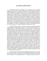
Table I. <strong>Black</strong> <strong>Swans</strong><br />
This exhibit shows all the black swans considered, ordered chronologically. A black swan is defined as a monthly return in the world<br />
market higher than or equal to 5% in absolute value. The world market is the MSCI index of developed markets between January 1970 <strong>and</strong><br />
December 1987, <strong>and</strong> the MSCI index of both developed <strong>and</strong> emerging markets between January 1988 <strong>and</strong> December 2009. For countries,<br />
all 99 black swans are relevant; for industries, only the 38 black swans after (<strong>and</strong> including) February 1998 are relevant. All returns in<br />
dollars <strong>and</strong> in %.<br />
Date <strong>Return</strong> Date <strong>Return</strong> Date <strong>Return</strong> Date <strong>Return</strong><br />
Nov/73 –12.9 May/84 –7.4 Dec/91 7.4 Nov/01 6.1<br />
Jul/74 –5.8 Aug/84 10.1 Mar/93 5.7 Jun/02 –6.1<br />
Aug/74 –9.5 Jan/85 5.6 Nov/93 –5.2 Jul/02 –8.4<br />
Sep/74 –9.2 May/85 5.2 Dec/93 5.4 Sep/02 –11.0<br />
Oct/74 9.7 Oct/85 5.4 Jan/94 6.6 Oct/02 7.4<br />
Jan/75 14.7 Nov/85 5.6 Nov/96 5.3 Nov/02 5.5<br />
Feb/75 9.0 Feb/86 9.0 May/97 6.0 Apr/03 8.9<br />
Jul/75 –5.4 Mar/86 9.8 Jun/97 5.1 May/03 5.8<br />
Oct/75 7.0 Aug/86 8.8 Aug/97 –7.0 Oct/03 6.1<br />
Jan/76 9.0 Jan/87 11.8 Sep/97 5.3 Dec/03 6.3<br />
Dec/76 7.6 Mar/87 6.2 Oct/97 –6.0 Nov/04 5.5<br />
Jul/78 7.3 Apr/87 5.9 Feb/98 6.8 Sep/07 5.4<br />
Oct/79 –7.3 Aug/87 5.9 Aug/98 –14.0 Jan/08 –8.2<br />
Jan/80 6.1 Oct/87 –17.0 Oct/98 9.1 Apr/08 5.7<br />
Mar/80 –10.6 Feb/88 5.8 Nov/98 6.1 Jun/08 –8.2<br />
Apr/80 6.7 Aug/88 –5.5 Oct/99 5.1 Sep/08 –12.5<br />
May/80 5.1 Oct/88 6.6 Dec/99 8.3 Oct/08 –19.8<br />
Sep/81 –7.4 Jul/89 11.3 Jan/00 –5.4 Nov/08 –6.5<br />
Feb/82 –6.0 May/90 10.4 Sep/00 –5.5 Feb/09 –9.7<br />
Apr/82 5.0 Aug/90 –9.4 Nov/00 –6.2 Mar/09 8.3<br />
Aug/82 7.4 Sep/90 –10.4 Feb/01 –8.4 Apr/09 11.9<br />
Oct/82 7.0 Oct/90 9.2 Mar/01 –6.7 May/09 10.1<br />
Nov/82 5.4 Feb/91 9.4 Apr/01 7.3 Jul/09 8.8<br />
Apr/83 7.2 Jun/91 –6.1 Sep/01 –9.1<br />
79<br />
II. Data <strong>and</strong> Methodology<br />
In this section, we first describe our data, define a black<br />
swan from an empirical perspective, <strong>and</strong> briefly discuss the<br />
black swans we consider. We then describe the methodology<br />
we use to assess the usefulness of beta as a measure of risk<br />
<strong>and</strong> as a tool for portfolio selection, focusing here on the<br />
main aspects <strong>and</strong> leaving some details for the next section.<br />
A. Data <strong>and</strong> <strong>Black</strong> <strong>Swans</strong><br />
Our sample consists of the entire MSCI database of<br />
countries <strong>and</strong> industries. We consider monthly returns<br />
on 47 countries (23 developed <strong>and</strong> 24 emerging) <strong>and</strong> 57<br />
industries (based on companies from both developed <strong>and</strong><br />
emerging markets) over the whole sample period available<br />
for each. Although not all series start at the same time, in all<br />
cases the data goes through December 2009. Exhibit A1 in<br />
the appendix shows all the countries <strong>and</strong> industries in our<br />
sample, the month in which the return data begins for each of<br />
them, <strong>and</strong> some summary statistics. All monthly returns are<br />
in dollars <strong>and</strong> account for both capital gains <strong>and</strong> dividends.<br />
Our benchmark portfolio, used both to determine the<br />
black swans we consider <strong>and</strong> to play the role of the passive<br />
investment when evaluating our beta-based strategy, is the<br />
MSCI world (equity) market index. Due to data availability,<br />
between January 1970 <strong>and</strong> December 1987 we use a world<br />
market portfolio consisting only of developed markets; from<br />
that point on, between January 1988 <strong>and</strong> December 2009, we<br />
use a world market portfolio consisting of both developed<br />
<strong>and</strong> emerging markets. As is the case with the rest of our<br />
data, the returns of the world market portfolio are in dollars<br />
<strong>and</strong> account for both capital gains <strong>and</strong> dividends.
80 Journal of Applied Finance – No. 2, 2012<br />
The first step in our inquiry is to identify the relevant<br />
black swans. Taleb (2007) defines a black swan as an event<br />
with three attributes: 1) It is an outlier, lying outside the<br />
realm of regular expectations because nothing in the past<br />
can convincingly point to its occurrence; 2) it carries an<br />
extreme impact; <strong>and</strong> 3) despite being an outlier, plausible<br />
explanations for its occurrence can be found after the fact,<br />
thus giving it the appearance that it can be explainable <strong>and</strong><br />
predictable. In short, a black swan has three characteristics:<br />
rarity, extreme impact, <strong>and</strong> retrospective predictability.<br />
This definition is illustrative but not operational. We<br />
therefore arbitrarily define a black swan as a monthly return<br />
in the world market higher than or equal to 5% in absolute<br />
value. Because we need to compute betas <strong>and</strong> we do so with<br />
a minimum of 36 months, we look for black swans only<br />
during the January 1973 to December 2009 period; that is,<br />
excluding the first three years of data. Given our definition,<br />
we find a total of 99 black swans, all of which are reported<br />
on Table I. All these black swans are relevant for our<br />
analysis across countries, but given that the sample period<br />
for industries is shorter than that for countries, only those<br />
black swans after (<strong>and</strong> including) February 1998 are relevant<br />
for our analysis across industries. 2<br />
In the case of countries, of the 99 black swans we identify,<br />
63 are positive (monthly returns higher than or equal to 5%)<br />
<strong>and</strong> 36 are negative (monthly returns lower than or equal<br />
to –5%). Positive <strong>and</strong> negative black swans average 7.3%<br />
<strong>and</strong> –8.6%. A runs test cannot reject the null hypothesis of<br />
r<strong>and</strong>omness (at a 5% confidence level, the test statistic of<br />
-0.62 is within the critical values of ±1.96), indicating that a<br />
positive or negative black swan has no information useful to<br />
determine the sign of the next black swan.<br />
In the case of industries, due to their shorter history, only<br />
38 of the 99 black swans are relevant, 21 of which are positive<br />
(averaging 7.2%) <strong>and</strong> 17 negative (averaging –9.1%). Again,<br />
a runs test indicates that black swans are unpredictable in<br />
sign (at at 5% confidence level, the test statistic of -1.59 is<br />
within the critical values of ±1.96), with the occurrence of<br />
one carrying no information about the sign of the next.<br />
The black swans in the sample are dependent on our<br />
definition for these events. It may be argued that black<br />
swans are very rare events, <strong>and</strong> that observing as many as<br />
we do in our sample is not consistent with such definition.<br />
The point is well taken. Our focus is on outliers or large<br />
market fluctuations, which many investors nowadays refer<br />
to as black swans. Importantly, there is no operational or<br />
quantitative definition of a black swan, which makes all<br />
definitions rather arbitrary; ours is no exception.<br />
2<br />
The return data for industries starts in January 1995, but again we exclude<br />
the first three years to allow for the estimation of betas. Thus, for industries,<br />
we look for black swans during the January 1998 to December 2009 period<br />
<strong>and</strong> we find the first on February 1998.<br />
It may be argued that a monthly fluctuation of |5%| in the<br />
world market is not large enough to qualify as a black swan.<br />
When choosing |5%| as the minimum monthly return to define<br />
a black swan, we attempted to strike a balance between two<br />
things: On the one h<strong>and</strong>, we did not want to end up with a<br />
sample with so many black swans that they could hardly be<br />
thought of as large <strong>and</strong> unexpected; on the other h<strong>and</strong>, we<br />
wanted to end up with a sample with enough black swans<br />
so that we could have many events to average across. To<br />
illustrate, if we had defined blacks swans as monthly returns<br />
in the world market of at least |10%|, we would have had<br />
only 15 events (8 negative <strong>and</strong> 7 positive) between January<br />
1973 <strong>and</strong> December 2009, relevant for countries; <strong>and</strong> only 6<br />
events (4 negative <strong>and</strong> 2 positive) between January 1998 <strong>and</strong><br />
December 2009, relevant for industries.<br />
B. Methodology<br />
In order to determine whether beta is a useful measure<br />
of risk, we assess the impact of negative black swans on<br />
diversified portfolios of countries <strong>and</strong> industries sorted by<br />
beta. More precisely, we explore whether high-beta portfolios<br />
fall more than low-beta portfolios when the market declines<br />
substantially, as theory would lead us to expect. 3<br />
In a nutshell, our procedure is as follows. Every time a<br />
negative black swan hits the market we estimate betas for<br />
each country in our sample on the basis of the 60 months<br />
previous to, but not including, the black swan month. 4 We<br />
then rank all countries by those betas; split them into four<br />
portfolios, one containing the high-beta countries, another<br />
containing the low-beta countries, <strong>and</strong> two portfolios in<br />
between; <strong>and</strong> calculate the return of each portfolio for the<br />
black swan month as an equally-weighted average of the<br />
returns of the countries in each portfolio during that month. 5<br />
This yields one return for each of the four portfolios for each<br />
negative black swan, <strong>and</strong> we finally average the returns of<br />
each portfolio across all negative black swans. This yields<br />
3<br />
Some may argue that exploring this issue is pointless because theory does<br />
lead to expect a positive relationship between beta <strong>and</strong> returns. Needless<br />
to say, Fama <strong>and</strong> French (1992) <strong>and</strong> a vast literature both before <strong>and</strong> after<br />
them report evidence inconsistent with this expectation. In other words,<br />
what theory may lead us to expect may or may not be what the data shows,<br />
<strong>and</strong> in the case of beta, there is a huge amount of evidence of both sides of<br />
the fence. Hence, we want to explore with our data, focus, <strong>and</strong> methodology<br />
whether there is in fact a positive relationship between beta <strong>and</strong> returns.<br />
4<br />
When the data does not allow for the estimation of 60-month betas, we<br />
estimate them with as many months as possible but never with less than<br />
36 months. All betas are estimated relative to the world market portfolio.<br />
5<br />
Whenever possible we allocate the same number of countries to each of<br />
the four portfolios. When this is not possible, we allocate the same number<br />
of countries to the riskiest <strong>and</strong> the least risky portfolios, <strong>and</strong> the rest of the<br />
countries to the two portfolios in the middle, always trying to keep the four<br />
portfolios as similar as possible in terms of the number of countries in each.
Estrada & Vargas – <strong>Black</strong> <strong>Swans</strong>, <strong>Beta</strong>, <strong>Risk</strong>, <strong>and</strong> <strong>Return</strong><br />
the average decline for the riskiest (high-beta) portfolio, the<br />
least risky (low-beta) portfolio, <strong>and</strong> the two portfolios in<br />
between.<br />
For reasons to be discussed below, we repeat this whole<br />
procedure also for positive black swans. And we finally<br />
repeat it again, for both negative <strong>and</strong> positive black swans,<br />
for our sample of industries. At the end of this first step we<br />
are able to assess whether beta is a good measure of risk<br />
when the latter is thought of as exposure to the downside<br />
during turbulent periods. Throughout this analysis, our focus<br />
is on economic (rather than statistical) significance.<br />
In our second step, we assess whether beta is a valuable<br />
tool for portfolio selection. To this purpose we devise<br />
an investable strategy based on beta that also accounts<br />
for the well-known pattern of mean reversion; that is, the<br />
tendency of equity markets to revert to their long-term<br />
mean, as documented by Siegel (2008) <strong>and</strong> many others. In<br />
the presence of mean reversion we would expect markets<br />
to eventually rise after negative black swans <strong>and</strong> fall after<br />
positive black swans. In fact, we would expect high-beta<br />
portfolios to rise more than low-beta portfolios after negative<br />
black swans; <strong>and</strong> low-beta portfolios to decline less than<br />
high-beta portfolios after positive black swans.<br />
This reasoning leads us to the following simple strategy<br />
(which we describe only for countries because it is similar<br />
for industries): After negative black swans, invest in a<br />
portfolio of high-beta countries, thus obtaining exposure<br />
to the countries expected to rise the most; after positive<br />
black swans, invest in a portfolio of low-beta countries, thus<br />
obtaining exposure to the countries expected to fall the least;<br />
<strong>and</strong> between black swans, simply hold whatever portfolio<br />
was formed after the last black swan.<br />
In order to implement this strategy, right after each black<br />
swan we estimate betas for all countries; rank all countries<br />
by those betas; split them into four portfolios, one containing<br />
the high-beta countries, another the low-beta countries, <strong>and</strong><br />
two portfolios in between; <strong>and</strong> invest in the portfolio of highbeta<br />
countries or low-beta countries depending on the sign<br />
of the black swan just observed. 6 The benchmark against<br />
which we compare this strategy is a passive (buy-<strong>and</strong>-hold)<br />
investment in the world market portfolio.<br />
Note that when consecutive black swans are of different<br />
sign, we switch from a high-beta portfolio to a low-beta<br />
6<br />
As before, whenever possible we allocate the same number of countries<br />
to each portfolio. When this is not possible, we allocate the same number<br />
of countries to the riskiest <strong>and</strong> the least-risky portfolios, <strong>and</strong> the rest of the<br />
countries to the two portfolios in the middle, always trying to keep the four<br />
portfolios as similar as possible in terms of the number of countries in each.<br />
Also as before, we estimate betas relative to the world market portfolio <strong>and</strong><br />
with as many months as possible, but never with less than 36 months or<br />
more than 60 months. The only difference with respect to what we do in our<br />
first step is that in this second step we estimate all betas as of the end of (that<br />
is, including) the black swan month.<br />
81<br />
portfolio, or the other way around. Also, note that even if<br />
consecutive black swans are of the same sign we may still<br />
rebalance our portfolio. This is the case simply because<br />
betas change over time, <strong>and</strong> which are the countries with the<br />
highest <strong>and</strong> lowest betas may change between black swans.<br />
In other words, we make sure that we are properly exposed<br />
to the riskiest or least risky countries after each black swan.<br />
Everything we just described for countries we then repeat<br />
for industries. At the end of this second step we will be able<br />
to assess the merits of our strategy relative to a passive<br />
investment in the world market, <strong>and</strong>, therefore, whether beta<br />
is a valuable tool for portfolio selection. As in our first step,<br />
our focus is on economic (rather than statistical) significance.<br />
III. Evidence<br />
In this section we first assess the merits of beta as a measure<br />
of risk <strong>and</strong> then as a tool for portfolio selection, in both cases<br />
focusing on countries. Subsequently, as a robustness test, we<br />
evaluate beta on both counts by focusing on industries.<br />
A. <strong>Beta</strong> As a Measure of <strong>Risk</strong> – Countries<br />
The first step in our inquiry is to ask whether beta is a good<br />
measure of risk, particularly when the latter is thought of<br />
as exposure to large <strong>and</strong> unexpected market declines. Chan<br />
<strong>and</strong> Lakonishok (1993) suggest that extensive conversations<br />
with money managers indicate that their main concern is<br />
downside risk. Furthermore, Grundy <strong>and</strong> Malkiel (1996)<br />
suggest that most investors think of risk as the possibility<br />
of losing money in a declining market. Our question is,<br />
precisely, whether beta is a proper measure of risk in this<br />
context.<br />
Following the methodology outlined in Section II, we<br />
explore the performance of country portfolios sorted by<br />
beta when negative black swans hit the market. Because we<br />
estimate betas on the basis of the 36-to-60 months previous<br />
to, but not including, the black swan months, we are able to<br />
determine the impact of large market declines on existing<br />
portfolios of high-beta <strong>and</strong> low-beta countries.<br />
As mentioned in Section I, during the relevant sample<br />
period there are 36 negative black swans as measured by<br />
monthly declines in the world market portfolio, averaging an<br />
8.6% fall. Our question, then, is whether high-beta portfolios<br />
fell, on average across all 36 events, more than low-beta<br />
portfolios; our results are summarized in Panel A of Table II.<br />
Across all 36 negative black swans, high-beta portfolios<br />
(P1) <strong>and</strong> low-beta portfolios (P4) have average betas of 1.50<br />
<strong>and</strong> 0.54. P2 <strong>and</strong> P3, the two portfolios in between, have<br />
average betas of 1.10 <strong>and</strong> 0.88. The decline in average betas<br />
from P1 to P4 is of course by construction; that is, right<br />
before each black swan countries were ranked by beta, the<br />
25% with highest betas were assigned to P1, the 25% with
82 Journal of Applied Finance – No. 2, 2012<br />
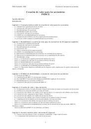
Table II. <strong>Beta</strong> <strong>and</strong> <strong>Risk</strong> – Countries<br />
This exhibit shows, in panel A, the average beta <strong>and</strong> average decline of the four country portfolios considered across 36 negative black<br />
swans; <strong>and</strong> in panel B, the average beta <strong>and</strong> average rise of those portfolios across 63 positive black swans. P1 <strong>and</strong> P4 denote the portfolios<br />
of high-beta <strong>and</strong> low-beta countries, <strong>and</strong> P2 <strong>and</strong> P3 two portfolios in between. The world market <strong>and</strong> the black swans considered are those<br />
described on Table I.<br />
Panel A. Negative <strong>Black</strong> <strong>Swans</strong><br />
World P1 P2 P3 P4 P1-P4<br />
<strong>Beta</strong> 1.00 1.50 1.10 0.88 0.54<br />
<strong>Return</strong> –8.6% –10.6% –9.2% –8.2% –7.1% –3.5%<br />
Panel B. Positive <strong>Black</strong> <strong>Swans</strong><br />
World P1 P2 P3 P4 P1-P4<br />
<strong>Beta</strong> 1.00 1.42 1.05 0.86 0.53<br />
<strong>Return</strong> 7.3% 9.8% 7.1% 7.1% 5.4% 4.4%<br />
the next-highest betas to P2, <strong>and</strong> so forth.<br />
In terms of returns, <strong>and</strong> again averaging across all 36<br />
events, the relationship between beta <strong>and</strong> return is strictly<br />
negative <strong>and</strong> monotonic. On average, high-beta portfolios<br />
fell by 10.6% <strong>and</strong> low-beta portfolios by 7.1%, in both<br />
cases relative to a decline of 8.6% for the world market. In<br />
other words, on average, high-beta portfolios fell 200bps<br />
more than the market, <strong>and</strong> low-beta portfolios fell 150bps<br />
less than the market. The 350bps monthly spread between<br />
P1 <strong>and</strong> P4 is, needless to say, substantial from an economic<br />
point of view. 7 As theory would lead us to expect, then, beta<br />
appears to properly capture the risk that concerns money<br />
managers <strong>and</strong> investors in general; that is, exposure to large<br />
<strong>and</strong> unexpected market declines.<br />
Panel B of Table II shows the performance of high-beta<br />
<strong>and</strong> low-beta portfolios when 63 positive black swans, with<br />
an average rise of 7.3%, hit the market. On average across all<br />
63 events, high-beta portfolios rose by 9.8% (250bps more<br />
than the market) <strong>and</strong> low-beta portfolios by 5.4% (190bps<br />
less than the market). The 440bps spread between P1 <strong>and</strong> P4<br />
is, as was the case for negative black swans, substantial from<br />
an economic point of view. 8<br />
Importantly for the strategy we evaluate below, note<br />
that Table II shows that when negative black swans hit the<br />
market, high-beta portfolios fall the most; that is, their prices<br />
are those punished most severely. On the other h<strong>and</strong>, when<br />
positive black swans hit the market, low-beta portfolios rise<br />
the least; that is, their price run-ups are the least excessive.<br />
We will get back to these two facts below.<br />
7<br />
Interestingly, during October 2008 (our largest negative black swan, when<br />
the world market dropped 19.8%), the high-beta portfolio fell by 30.8% <strong>and</strong><br />
the low-beta portfolio by 19.7%, for a very substantial spread of 1,110bps.<br />
8<br />
Although the table shows P2 <strong>and</strong> P3 as rising by the same amount when the<br />
results are rounded to one decimal, P2’s average rise of 7.14% is actually<br />
slightly higher than P3’s average rise of 7.10%.<br />
B. <strong>Beta</strong> As a Tool for Portfolio Selection –<br />
Countries<br />
The second step in our inquiry is to ask whether beta<br />
is a valuable tool for portfolio selection by following<br />
the methodology outlined in Section II. We kick-off the<br />
horse race by investing $100 in our strategy <strong>and</strong> in the<br />
world market portfolio (the passive benchmark) after the<br />
first relevant black swan hits the market, on November<br />
1973. More precisely, at the very beginning of December<br />
1973, we estimate betas for all countries, rank countries<br />
by those betas, <strong>and</strong> split them into four portfolios. 9 Given<br />
that November 1973 is a negative black swan, <strong>and</strong> that in<br />
the presence of mean reversion we would expect stocks to<br />
eventually rebound from this large decline, we invest $100<br />
in the portfolio of high-beta countries (<strong>and</strong> at the same time<br />
another $100 in the world market portfolio), thus obtaining<br />
exposure to the countries expected to rebound the most.<br />
We hold this (high-beta) portfolio until the next black<br />
swan hits the market (July 1974), <strong>and</strong> then at the very<br />
beginning of August 1974 we again estimate betas, rank<br />
countries by those betas, <strong>and</strong> split them into four portfolios.<br />
Given that August 1974 is another negative black swan, we<br />
position our accumulated funds in the high-beta portfolio<br />
again. 10 We keep repeating this process until the end of our<br />
sample period (December 2009), at which point we evaluate<br />
the performance of our strategy <strong>and</strong> that of the passive<br />
benchmark. The results of this evaluation are summarized in<br />
Table III <strong>and</strong> in Exhibits A2 <strong>and</strong> A3 in the appendix.<br />
9<br />
Importantly, note that all our portfolios are built solely on the basis of<br />
information that would have been available to investors at the time of<br />
construction; therefore, ours is an investable strategy.<br />
10<br />
The first time we position our funds in a low-beta portfolio is after the<br />
October 1974 positive black swan, <strong>and</strong> we do so, as discussed before, in<br />
order to gain exposure to the countries expected to fall the least.
Estrada & Vargas – <strong>Black</strong> <strong>Swans</strong>, <strong>Beta</strong>, <strong>Risk</strong>, <strong>and</strong> <strong>Return</strong><br />
Table III. <strong>Beta</strong> <strong>and</strong> Performance – Countries<br />
This exhibit summarizes the performance of our strategy (Strategy) <strong>and</strong> that of the passive investment in the world market portfolio<br />
(World) over the 433 months between December 1973 <strong>and</strong> December 2009. For both series of monthly dollar returns panel A shows<br />
the arithmetic mean return (AM), geometric mean return (GM), st<strong>and</strong>ard deviation (SD), beta with respect to the world market (<strong>Beta</strong>),<br />
semideviation for a benchmark of 0% (SSD), minimum (Min) <strong>and</strong> maximum (Max) return, <strong>and</strong> coefficients of st<strong>and</strong>ardized skewness<br />
(SSkw) <strong>and</strong> st<strong>and</strong>ardized kurtosis (SKrt). Panel B shows the annualized st<strong>and</strong>ard deviation (ASD) <strong>and</strong> annualized geometric mean return<br />
(AGM); the terminal value (TV) at the end of December 2009 of $100 invested at the beginning of December 1973; the terminal value of<br />
$100 invested at AGM after any hypothetical period of 10 (TV10), 20 (TV20), <strong>and</strong> 30 (TV30) years; <strong>and</strong> risk-adjusted returns based on<br />
SD (RAR1=AM/SD) <strong>and</strong> SSD (RAR2=AM/SSD).<br />
Panel A. Performane Measures<br />
AM GM SD <strong>Beta</strong> SSD Min Max SSkw SKrt<br />
World 0.9% 0.8% 4.4% 1.00 2.9% –19.8% 14.7% –4.9 8.2<br />
Strategy 1.3% 1.1% 5.5% 0.96 3.6% –31.2% 21.7% –8.2 22.8<br />
Panel B. Performance Measures (Continued)<br />
ASD AGM TV TV10 TV20 TV30 RAR1 RAR2<br />
World 15.2% 10.1% $3,210 $262 $684 $1,788 0.21 0.31<br />
Strategy 19.2% 14.4% $12,834 $384 $1,474 $5,661 0.23 0.35<br />
83<br />
Panel A shows that over the evaluation period of 433<br />
months, our strategy delivered a higher arithmetic <strong>and</strong><br />
geometric mean return than the passive investment, <strong>and</strong> it did<br />
so with somewhat higher risk, regardless of whether the latter<br />
is measured by the st<strong>and</strong>ard deviation, the semideviation, the<br />
minimum return, or the fatness of the tails as measured by<br />
the coefficient of st<strong>and</strong>ardized kurtosis. 11 As shown in Panel<br />
B, the annualized volatility of our strategy was 4 percentage<br />
points higher than that of the passive investment (19.2%<br />
versus 15.2%).<br />
Panel B also shows that our strategy delivered an<br />
annualized return of 14.4%, outperforming the 10.1%<br />
annualized return of the passive investment by a very<br />
substantial 430bps a year. The $100 invested in our strategy<br />
at the beginning of December 1973 would have turned<br />
into $12,834 by December 2009, almost exactly four times<br />
as much as the $3,210 we would have obtained from the<br />
passive investment. 12 There is something to be said about<br />
a strategy that outperforms a passive investment by such a<br />
substantial margin.<br />
Finally, Panel B suggests that our strategy also<br />
outperformed the passive investment in terms of riskadjusted<br />
returns, regardless of whether risk is measured<br />
by volatility or downside volatility. If risk is measured<br />
by the st<strong>and</strong>ard deviation, the 0.23 risk-adjusted return<br />
11<br />
The semideviation measures volatility below, but not above, any chosen<br />
benchmark. All semideviations in this article are calculated for a benchmark<br />
of 0% <strong>and</strong> therefore measure volatility below that benchmark. For a<br />
practical introduction to the semideviation, see Estrada (2006).<br />
12<br />
Panel B also shows the terminal value of $100 invested at the annualized<br />
returns (AGM) shown in this panel after any hypothetical investment period<br />
of 10, 20, <strong>and</strong> 30 years.<br />
of our strategy outpaced (by 13%) the 0.21 of the passive<br />
investment; if risk is measured by the semideviation instead,<br />
the 0.35 risk-adjusted return of our strategy also outpaced<br />
(by 12.2%) the 0.31 of the passive investment. That being<br />
said, a test for a difference in Sharpe ratios does not reject<br />
the equality of risk-adjusted returns, at least when risk is<br />
measured by volatility. 13<br />
A few remarks are in order. First, as discussed before,<br />
note that our strategy seeks to be exposed to high-beta<br />
countries when the market is expected to rise (after negative<br />
black swans), <strong>and</strong> to low-beta countries when the market<br />
is expected to fall (after positive black swans). Note that,<br />
at the same time, our strategy tends to buy the countries<br />
whose prices have fallen the most or risen the least. This<br />
is the case because we form our portfolios after observing<br />
black swans. Table II shows that the portfolios that fall the<br />
most during negative black swans are those with high beta;<br />
these are precisely the portfolios we buy after negative black<br />
swans in order to profit the most from the expected recovery.<br />
Similarly, Table II shows that the portfolios that rise the<br />
least during positive black swans are those with low beta;<br />
<strong>and</strong> these are precisely the portfolios we buy after positive<br />
black swans in order to minimize the impact of the expected<br />
downturn. Thus, our strategy tends to buy relatively cheap<br />
assets in the sense that their prices have fallen the most or<br />
risen the least.<br />
It is important to note that we tend to buy the countries<br />
whose prices have fallen the most or risen the least, although<br />
we do not necessarily do that in every case. In order to do<br />
that, instead of focusing on beta we would have to focus<br />
13<br />
This conclusion follows from the Jobson-Korkie-Memmel test; see<br />
Memmel (2003).
84 Journal of Applied Finance – No. 2, 2012<br />
Table IV. <strong>Beta</strong> <strong>and</strong> <strong>Risk</strong> – Industries<br />
This exhibit shows, in panel A, the average beta <strong>and</strong> average decline of the four industry portfolios considered across 17 negative black<br />
swans; <strong>and</strong> in panel B, the average beta <strong>and</strong> average rise of those portfolios across 21 positive black swans. P1 <strong>and</strong> P4 denote the portfolios<br />
of high-beta <strong>and</strong> low-beta industries, <strong>and</strong> P2 <strong>and</strong> P3 two portfolios in between. The world market <strong>and</strong> the black swans considered are those<br />
described on Table I.<br />
Panel A. Negative <strong>Black</strong> <strong>Swans</strong><br />
World P1 P2 P3 P4 P1-P4<br />
<strong>Beta</strong> 1.00 1.49 1.03 0.81 0.42<br />
<strong>Return</strong> –9.1% –11.4% –9.4% –8.6% –5.3% –6.1%<br />
Panel B. Positive <strong>Black</strong> <strong>Swans</strong><br />
World P1 P2 P3 P4 P1-P4<br />
<strong>Beta</strong> 1.00 1.48 1.04 0.83 0.47<br />
<strong>Return</strong> 7.2% 9.4% 7.8% 6.3% 4.0% 5.4%<br />
on returns. However, our goal in this article is to evaluate<br />
beta as a tool for portfolio selection, <strong>and</strong>, therefore, we<br />
base our strategy solely on this magnitude. That being said,<br />
Table II shows that high-beta countries tend to be (though<br />
not necessarily are in every case) those whose prices fall the<br />
most during negative black swans; <strong>and</strong> low-beta countries<br />
tend to be (but again not necessarily are in every case) those<br />
whose prices rise the least during positive black swans.<br />
Secondly, as discussed earlier, our strategy buys low-beta<br />
stocks after positive black swans in order to minimize the<br />
impact of a market that is expected to decline. Arguably,<br />
in these circumstances we could enhance the returns of our<br />
strategy (<strong>and</strong> most likely lower its volatility) by parking our<br />
accumulated funds in cash or bonds rather than investing<br />
them in a low-beta portfolio. Yet again, because of our focus<br />
in on beta, we decided to implement the latter.<br />
Thirdly, the figures on Table III do not account for the<br />
transaction costs of our strategy or those of the passive<br />
investment. Although typically ignored, a passive<br />
investment would still incur in the annual cost of the relevant<br />
index fund or ETF (the world market portfolio is currently<br />
investable through at least two ETFs whose annual expense<br />
ratio is around 30-35bps). Our strategy, which rebalances<br />
the portfolio after each black swan, would have incurred in<br />
higher transaction costs, but nothing even remotely close<br />
to the 430bps annual outperformance over the passive<br />
investment.<br />
Finally, although we do not test formally for mean<br />
reversion, our results imply that it is present in the data. We<br />
do not explore this issue further simply because it is not one<br />
of our goals in this article. That being said, our beta-based<br />
strategy is expected to outperform the passive investment<br />
only in the presence of mean reversion, not in the presence<br />
of r<strong>and</strong>om walks. We take no preliminary view on whether<br />
either process is present in the data; we simply run a horse<br />
race between our strategy <strong>and</strong> a passive investment, find<br />
that our strategy outperforms, <strong>and</strong> highlight that our results<br />
imply the presence of mean reverting returns.<br />
C. Robustness Test – Industries<br />
The results discussed so far support beta both as a measure<br />
of risk <strong>and</strong> as a tool for portfolio selection. However, as is<br />
usually the case with empirical studies, one might wonder<br />
whether the results would have been more or less supportive<br />
if we had defined black swans, or estimated betas, or formed<br />
portfolios in a different way. Rather than replicating all of<br />
our work for countries after defining black swans differently,<br />
or estimating betas over a longer or shorter period of time,<br />
or forming portfolios using another criterion, we chose to<br />
repeat all of our work for countries on an entirely different<br />
dataset. Here is where the 57 industries mentioned in Section<br />
II come in.<br />
As a robustness test, everything we run for countries we<br />
re-run for industries. As mentioned in Section II, there are<br />
17 negative black swans during the relevant (January 1998<br />
to December 2009) period, averaging –9.1%. Panel A of<br />
Table IV summarizes the results of our new inquiry about<br />
the usefulness of beta as a measure of risk. As the exhibit<br />
shows, across all 17 events, high-beta portfolios (P1) <strong>and</strong><br />
low-beta portfolios (P4) have average betas of 1.49 <strong>and</strong> 0.42.<br />
P2 <strong>and</strong> P3, the two portfolios in between, have average betas<br />
of 1.10 <strong>and</strong> 0.81.<br />
In terms of returns, averaging across all 17 events,<br />
the relationship between beta <strong>and</strong> return is again strictly<br />
negative <strong>and</strong> monotonic. On average, high-beta portfolios<br />
fell by 11.4% <strong>and</strong> low-beta portfolios by 5.3%, in both cases<br />
relative to a decline of 9.1% for the world market. In other<br />
words, on average, high-beta portfolios fell 230bps more than<br />
the market, <strong>and</strong> low-beta portfolios fell 380bps less than the<br />
market. The 610bps monthly spread between P1 <strong>and</strong> P4 is<br />
obviously substantial from an economic point of view. Thus,
Estrada & Vargas – <strong>Black</strong> <strong>Swans</strong>, <strong>Beta</strong>, <strong>Risk</strong>, <strong>and</strong> <strong>Return</strong><br />
Table V. <strong>Beta</strong> <strong>and</strong> Performance – Industries<br />
This exhibit summarizes the performance of our strategy (Strategy) <strong>and</strong> that of the passive investment in the world market portfolio<br />
(World) over the 142 months between March 1998 <strong>and</strong> December 2009. For both series of monthly dollar returns panel A shows the<br />
arithmetic mean return (AM), geometric mean return (GM), st<strong>and</strong>ard deviation (SD), beta with respect to the world market (<strong>Beta</strong>),<br />
semideviation for a benchmark of 0% (SSD), minimum (Min) <strong>and</strong> maximum (Max) return, <strong>and</strong> coefficients of st<strong>and</strong>ardized skewness<br />
(SSkw) <strong>and</strong> st<strong>and</strong>ardized kurtosis (SKrt). Panel B shows the annualized st<strong>and</strong>ard deviation (ASD) <strong>and</strong> annualized geometric mean return<br />
(AGM); the terminal value (TV) at the end of December 2009 of $100 invested at the beginning of March 1998; the terminal value of<br />
$100 invested at AGM after any hypothetical period of 10 (TV10), 20 (TV20), <strong>and</strong> 30 (TV30) years; <strong>and</strong> risk-adjusted returns based on<br />
SD (RAR1=AM/SD) <strong>and</strong> SSD (RAR2=AM/SSD).<br />
Panel A. Performance Measures<br />
AM GM SD <strong>Beta</strong> SSD Min Max SSkw SKrt<br />
World 0.4% 0.3% 4.9% 1.00 3.6% –19.8% 11.9% –4.2 4.4<br />
Strategy 0.6% 0.5% 5.1% 0.90 3.8% –25.1% 12.3% –6.7 13.5<br />
Panel B. Performance Measures (Cont.)<br />
ASD AGM TV TV10 TV20 TV30 RAR1 RAR2<br />
World 17.0% 3.8% $155 $145 $209 $303 0.09 0.12<br />
Strategy 17.7% 5.8% $195 $176 $309 $542 0.12 0.16<br />
85<br />
these results for industries strengthen the previous ones for<br />
countries <strong>and</strong> reinforce the fact that beta is a good measure<br />
of exposure to large <strong>and</strong> unexpected market declines.<br />
Panel B of Table IV summarizes the performance of highbeta<br />
<strong>and</strong> low-beta portfolios when 21 positive black swans,<br />
averaging 7.2%, hit the market. On average across all 21<br />
events, high-beta portfolios rose by 9.4% (220bps more than<br />
the market) <strong>and</strong> low-beta portfolios by 4.0% (320bps less<br />
than the market). The 540bps spread between P1 <strong>and</strong> P4 is<br />
again substantial from an economic point of view.<br />
Finally, Table IV shows that when negative black swans<br />
hit the market, high-beta portfolios fall the most; <strong>and</strong> when<br />
positive black swans hit the market, low-beta portfolios<br />
rise the least. As was the case for countries, then, the betabased<br />
strategy we evaluate immediately below benefits from<br />
buying assets whose prices have fallen the most or risen the<br />
least.<br />
The investable strategy, identical to that implemented<br />
before for countries but now applied to industries, again<br />
reacts to negative black swans by investing in high-beta<br />
portfolios, <strong>and</strong> to positive black swans by investing in lowbeta<br />
portfolios. The benchmark against which we compare<br />
the performance of this strategy is again a passive investment<br />
in the world market portfolio. Table V <strong>and</strong> Exhibit A4 in the<br />
appendix summarize the results of our new inquiry about the<br />
usefulness of beta as a tool for portfolio selection.<br />
As was the case for countries, Panel A shows that our<br />
strategy delivered a higher arithmetic <strong>and</strong> geometric mean<br />
return than the passive investment, <strong>and</strong> it did so with<br />
somewhat higher risk regardless of whether the latter is<br />
measured by the st<strong>and</strong>ard deviation, the semideviation,<br />
the minimum return, or the fatness of the tails as measured<br />
by the coefficient of st<strong>and</strong>ardized kurtosis. Importantly, as<br />
Panel B shows, our strategy had an annualized volatility less<br />
than one percentage point higher than the passive investment<br />
(17.7% versus 17.0%).<br />
Panel B also shows that our strategy delivered an<br />
annualized return of 5.8%, outperforming the 3.8% return<br />
delivered by the passive investment by 200bps a year. Thus,<br />
$100 invested in our strategy at the beginning of March<br />
1998 would have turned into $195 by December 2009, over<br />
25% more than the $155 we would have obtained from the<br />
passive investment.<br />
Finally, Panel B suggests that our strategy also<br />
outperformed the passive investment in terms of riskadjusted<br />
returns, regardless of whether risk is measured<br />
by volatility or downside volatility. If risk is measured<br />
by the st<strong>and</strong>ard deviation, the 0.12 risk-adjusted return of<br />
our strategy outpaced (by 35.4%) the 0.09 of the passive<br />
investment; if risk is measured by the semideviation instead,<br />
the 0.16 risk-adjusted return of our strategy also outpaced<br />
(by 32.6%) the 0.12 of the passive investment. 14 Thus, these<br />
results for industries again strengthen the previous ones for<br />
countries <strong>and</strong> reinforce the fact that beta is a valuable tool<br />
for portfolio selection.<br />
IV. An Assessment<br />
The debate on the usefulness of beta as a measure of risk,<br />
<strong>and</strong> on the CAPM as an appropriate model to estimate<br />
required returns, has been raging on for decades. No single<br />
14<br />
That being said, as before, the difference in risk-adjusted returns is not<br />
significant, at least when risk is measured by volatility, according to the<br />
Jobson-Korkie-Memmel test.
86 Journal of Applied Finance – No. 2, 2012<br />
paper can be expected to settle this controversy <strong>and</strong> ours is<br />
no exception. Reasonable people must ultimately balance<br />
the empirical arguments in favor of <strong>and</strong> against beta, <strong>and</strong><br />
our paper may be viewed as adding a straw that tilts a little,<br />
in favor of beta, the scale that weighs the evidence on this<br />
contentious issue.<br />
A distinctive characteristic of our approach is the context<br />
on which we evaluate beta. We do not focus on individual<br />
stocks but on diversified portfolios of countries <strong>and</strong><br />
industries. We do not start from the presumption that beta<br />
is a proper measure of risk but explore whether it properly<br />
captures exposure to the downside. And we do not test<br />
whether beta <strong>and</strong> returns are significantly related but devise<br />
a beta-based strategy <strong>and</strong> ask whether it outperforms a<br />
passive investment.<br />
Our evidence spans over 47 countries, 57 industries,<br />
<strong>and</strong> four decades <strong>and</strong> supports the usefulness of beta both<br />
as a measure of risk <strong>and</strong> as a tool for portfolio selection.<br />
High-beta portfolios do fall substantially more than lowbeta<br />
portfolios when the market is hit by negative black<br />
swans. The difference ranges from 350bps (for countries) to<br />
610bps (for industries) a month, clearly substantial from an<br />
economic point of view.<br />
Furthermore, an investable strategy that reacts to negative<br />
black swans by investing in high-beta portfolios, <strong>and</strong> to<br />
positive black swans by investing in low-beta portfolios,<br />
does outperform a passive investment in the world market.<br />
The difference in returns ranges from 200bps (for industries)<br />
to 430bps (for countries) a year, again substantial from an<br />
economic point of view.<br />
From the perspective we look at it, beta does seem to<br />
be a good measure of risk, at least in the sense of properly<br />
capturing the exposure to large <strong>and</strong> unexpected market<br />
declines that concerns portfolio managers <strong>and</strong> investors at<br />
large. And it does seem to be a valuable tool for portfolio<br />
selection, at least in the sense of selecting the portfolios<br />
expected to rise the most (after negative black swans) <strong>and</strong><br />
decline the least (after positive black swans), thus exposing<br />
investors to a strategy very likely to outperform a passive<br />
investment.<br />
All in all, our evidence supports beta both as a measure<br />
of risk <strong>and</strong> as a tool for portfolio selection. From a portfolio<br />
management perspective, then, we think it may be too early<br />
to discard this very controversial magnitude. In fact, from<br />
where we st<strong>and</strong>, beta does look alive <strong>and</strong> well.•<br />
Appendix<br />
Exhibit A1. Summary Statistics<br />
This exhibit shows, for the series of monthly returns, the arithmetic mean (AM), geometric mean (GM), <strong>and</strong> st<strong>and</strong>ard deviation (SD) of<br />
all the countries <strong>and</strong> industries in the sample, all calculated between the beginning (Start) <strong>and</strong> the end (Dec/2009) of each series’ sample<br />
period. All country <strong>and</strong> industry benchmarks are MSCI indices. <strong>Return</strong>s are in dollars <strong>and</strong> account for capital gains <strong>and</strong> dividends. All<br />
figures in %.<br />
Country AM GM SD Start Industry AM GM SD Start<br />
Developed Aerospace <strong>and</strong> Defense 1.0 0.8 5.9 Jan/95<br />
Australia 1.0 0.8 7.0 Jan/70 Air Freight <strong>and</strong> Logistics 0.8 0.6 5.6 Jan/95<br />
Austria 1.0 0.8 6.6 Jan/70 Airlines 0.4 0.2 6.5 Jan/95<br />
Belgium 1.1 0.9 6.0 Jan/70 Auto Components 0.5 0.3 6.0 Jan/95<br />
Canada 1.0 0.8 5.8 Jan/70 Automobiles 0.7 0.5 6.2 Jan/95<br />
Denmark 1.2 1.0 5.6 Jan/70 Beverages 0.8 0.7 4.5 Jan/95<br />
Finl<strong>and</strong> 1.2 0.8 9.4 Jan/88 Biotechnology 0.9 0.6 8.2 Jan/95<br />
France 1.1 0.9 6.5 Jan/70 Building Products 0.4 0.2 6.1 Jan/95<br />
Germany 1.0 0.8 6.3 Jan/70 Chemicals 0.8 0.7 5.4 Jan/95<br />
Greece 1.3 0.8 10.5 Jan/88 Commercial Banks 0.7 0.5 6.2 Jan/95<br />
Hong Kong 1.7 1.2 10.4 Jan/70 Commercial Services <strong>and</strong> Supplies 0.3 0.2 4.7 Jan/95<br />
Irel<strong>and</strong> 0.5 0.3 6.4 Jan/88 Communications Equipment 0.9 0.4 9.7 Jan/95<br />
Italy 0.8 0.5 7.3 Jan/70 Computers <strong>and</strong> Peripherals 1.1 0.8 8.1 Jan/95<br />
Japan 1.0 0.8 6.3 Jan/70 Construction <strong>and</strong> Engineering 0.5 0.3 6.4 Jan/95<br />
Netherl<strong>and</strong>s 1.2 1.0 5.6 Jan/70 Construction Materials 0.7 0.5 6.4 Jan/95<br />
New Zeal<strong>and</strong> 0.7 0.4 6.8 Jan/88 Containers <strong>and</strong> Packaging 0.2 0.0 6.0 Jan/95<br />
Norway 1.3 0.9 7.9 Jan/70 Distributors 0.0 –0.3 8.3 Jan/95<br />
Portugal 0.6 0.4 6.6 Jan/88 Diversified Financial Services 0.6 0.3 7.4 Jan/95<br />
Singapore 1.3 0.9 8.5 Jan/70 Diversified Telecommunication Sces. 0.5 0.4 5.6 Jan/95<br />
Spain 1.1 0.8 6.6 Jan/70 Electric Utilities 0.8 0.7 3.6 Jan/95<br />
Sweden 1.3 1.1 7.0 Jan/70 Electronic Equipment <strong>and</strong> Instruments 0.4 0.1 7.9 Jan/95<br />
Switzerl<strong>and</strong> 1.1 0.9 5.4 Jan/70 Electronic Equipment Manufacturers 0.8 0.5 6.6 Jan/95<br />
UK 1.0 0.8 6.5 Jan/70 Energy Equipment <strong>and</strong> Services 1.3 0.9 9.3 Jan/95<br />
USA 0.9 0.8 4.5 Jan/70 Food Products 0.8 0.7 3.8 Jan/95<br />
Emerging Food/Staples Retailers 0.6 0.5 3.7 Jan/95 (Continued)<br />
Argentina 2.5 1.3 16.1 Jan/88 Gas Utilities 0.8 0.8 4.2 Jan/95<br />
Brazil 2.9 1.7 15.4 Jan/88 Health Care Equipment <strong>and</strong> Support 0.9 0.8 4.4 Jan/95<br />
Chile 1.8 1.5 7.2 Jan/88 Health Care Providers <strong>and</strong> Services 0.7 0.5 6.0 Jan/95<br />
China 0.6 0.0 11.0 Jan/93 Hotels, Restaurants <strong>and</strong> Leisure 0.7 0.5 5.1 Jan/95<br />
Colombia 1.8 1.3 9.6 Jan/93 Household Durables 0.2 0.0 6.9 Jan/95<br />
Czech Rep. 1.6 1.2 8.7 Jan/95 Household Products 1.0 0.9 4.7 Jan/95
Hong Kong 1.7 1.2 10.4 Jan/70 Commercial Services <strong>and</strong> Supplies 0.3 0.2 4.7 Jan/95<br />
Irel<strong>and</strong> 0.5 0.3 6.4 Jan/88 Communications Equipment 0.9 0.4 9.7 Jan/95<br />
Italy 0.8 0.5 7.3 Jan/70 Computers <strong>and</strong> Peripherals 1.1 0.8 8.1 Jan/95<br />
Japan 1.0 0.8 6.3 Jan/70 Construction <strong>and</strong> Engineering 0.5 0.3 6.4 Jan/95<br />
Netherl<strong>and</strong>s 1.2 1.0 5.6 Jan/70 Construction Materials 0.7 0.5 6.4 Jan/95<br />
New Zeal<strong>and</strong> 0.7 0.4 6.8 Jan/88 Containers <strong>and</strong> Packaging 0.2 0.0 6.0 Jan/95<br />
Norway 1.3 0.9 7.9 Jan/70 Distributors 0.0 –0.3 8.3 Jan/95<br />
Portugal 0.6 0.4 6.6 Jan/88 Diversified Financial Services 0.6 0.3 7.4 Jan/95<br />
Estrada & Singapore<br />
Vargas – 1.3<br />
<strong>Black</strong> <strong>Swans</strong>,<br />
0.9<br />
<strong>Beta</strong>,<br />
8.5<br />
<strong>Risk</strong>,<br />
Jan/70 Diversified Telecommunication Sces 0.5 0.4 5.6 Jan/95<br />
<strong>and</strong> <strong>Return</strong><br />
Spain 1.1 0.8 6.6 Jan/70 Electric Utilities 0.8 0.7 3.6 Jan/95<br />
Sweden 1.3 1.1 Exhibit 7.0 Jan/70 A1. Summary Electronic Statistics Equipment (Continued)<br />
<strong>and</strong> Instruments 0.4 0.1 7.9 Jan/95<br />
Switzerl<strong>and</strong> 1.1 0.9 5.4 Jan/70 Electronic Equipment Manufacturers 0.8 0.5 6.6 Jan/95<br />
UK 1.0 0.8 6.5 Jan/70 Energy Equipment <strong>and</strong> Services 1.3 0.9 9.3 Jan/95<br />
Country AM GM SD Start Industry AM GM SD Start<br />
USA 0.9 0.8 4.5 Jan/70 Food Products 0.8 0.7 3.8 Jan/95<br />
Developed<br />
Emerging<br />
Aerospace<br />
Food/Staples<br />
<strong>and</strong><br />
Retailers<br />
Defense 1.0<br />
0.6<br />
0.8<br />
0.5<br />
5.9<br />
3.7<br />
Jan/95<br />
Jan/95<br />
Australia<br />
Argentina<br />
1.0<br />
2.5<br />
0.8<br />
1.3 16.1<br />
7.0 Jan/70<br />
Jan/88<br />
Air<br />
Gas<br />
Freight<br />
Utilities<br />
<strong>and</strong> Logistics 0.8<br />
0.8<br />
0.6<br />
0.8<br />
5.6<br />
4.2<br />
Jan/95<br />
Jan/95<br />
Austria<br />
Brazil<br />
1.0<br />
2.9<br />
0.8<br />
1.7 15.4<br />
6.6 Jan/70<br />
Jan/88<br />
Airlines<br />
Health Care Equipment <strong>and</strong> Support<br />
0.4<br />
0.9<br />
0.2<br />
0.8<br />
6.5<br />
4.4<br />
Jan/95<br />
Jan/95<br />
Belgium<br />
Chile<br />
1.1<br />
1.8<br />
0.9<br />
1.5<br />
6.0<br />
7.2<br />
Jan/70<br />
Jan/88<br />
Auto<br />
Health<br />
Components<br />
Care Providers <strong>and</strong> Services<br />
0.5<br />
0.7<br />
0.3<br />
0.5<br />
6.0<br />
6.0<br />
Jan/95<br />
Jan/95<br />
Canada<br />
China<br />
1.0<br />
0.6<br />
0.8<br />
0.0 11.0<br />
5.8 Jan/70<br />
Jan/93<br />
Automobiles<br />
Hotels, Restaurants <strong>and</strong> Leisure<br />
0.7<br />
0.7<br />
0.5<br />
0.5<br />
6.2<br />
5.1<br />
Jan/95<br />
Jan/95<br />
Denmark<br />
Colombia<br />
1.2<br />
1.8<br />
1.0<br />
1.3<br />
5.6<br />
9.6<br />
Jan/70<br />
Jan/93<br />
Beverages<br />
Household Durables<br />
0.8<br />
0.2<br />
0.7<br />
0.0<br />
4.5<br />
6.9<br />
Jan/95<br />
Jan/95<br />
Finl<strong>and</strong><br />
Czech Rep.<br />
1.2<br />
1.6<br />
0.8<br />
1.2<br />
9.4<br />
8.7<br />
Jan/88<br />
Jan/95<br />
Biotechnology<br />
Household Products<br />
0.9<br />
1.0<br />
0.6<br />
0.9<br />
8.2<br />
4.7<br />
Jan/95<br />
Jan/95<br />
France<br />
Egypt<br />
1.1<br />
2.0<br />
0.9<br />
1.5<br />
6.5<br />
9.8<br />
Jan/70<br />
Jan/95<br />
Building<br />
Industrial<br />
Products<br />
Conglomerates<br />
0.4<br />
0.7<br />
0.2<br />
0.5<br />
6.1<br />
6.3<br />
Jan/95<br />
Jan/95<br />
Germany<br />
Hungary<br />
1.0<br />
1.9<br />
0.8<br />
1.3 11.0<br />
6.3 Jan/70<br />
Jan/95<br />
Chemicals<br />
Information Technology Services<br />
0.8<br />
0.3<br />
0.7<br />
0.0<br />
5.4<br />
7.7<br />
Jan/95<br />
Jan/95<br />
Greece<br />
India<br />
1.3<br />
1.3<br />
0.8<br />
0.9<br />
10.5<br />
9.1<br />
Jan/88<br />
Jan/93<br />
Commercial<br />
Insurance<br />
Banks 0.7<br />
0.6<br />
0.5<br />
0.4<br />
6.2<br />
6.1<br />
Jan/95<br />
Jan/95<br />
Hong<br />
Indonesia<br />
Kong 1.7<br />
2.0<br />
1.2<br />
0.9<br />
10.4<br />
15.1<br />
Jan/70<br />
Jan/88<br />
Commercial<br />
Internet <strong>and</strong><br />
Services<br />
Catalogue<br />
<strong>and</strong><br />
Retail<br />
Supplies 0.3<br />
1.1<br />
0.2<br />
0.6<br />
4.7<br />
9.6<br />
Jan/95<br />
Jan/95<br />
Irel<strong>and</strong><br />
Israel<br />
0.5<br />
0.9<br />
0.3<br />
0.7<br />
6.4<br />
7.2<br />
Jan/88<br />
Jan/93<br />
Communications<br />
Internet Software<br />
Equipment<br />
<strong>and</strong> Services<br />
0.9<br />
1.7 –0.2<br />
0.4<br />
16.4<br />
9.7 Jan/95<br />
Jan/95<br />
Italy<br />
Jordan<br />
0.8<br />
0.5<br />
0.5<br />
0.4<br />
7.3<br />
5.4<br />
Jan/70<br />
Jan/88<br />
Computers<br />
Leisure Equipment<br />
<strong>and</strong> Peripherals<br />
<strong>and</strong> Products<br />
1.1<br />
0.3<br />
0.8<br />
0.1<br />
8.1<br />
5.1<br />
Jan/95<br />
Jan/95<br />
Japan<br />
Korea<br />
1.0<br />
1.2<br />
0.8<br />
0.6 11.4<br />
6.3 Jan/70<br />
Jan/88<br />
Construction<br />
Machinery<br />
<strong>and</strong> Engineering 0.5<br />
0.6<br />
0.3<br />
0.4<br />
6.4<br />
6.2<br />
Jan/95<br />
Jan/95<br />
Netherl<strong>and</strong>s<br />
Malaysia<br />
1.2<br />
1.0<br />
1.0<br />
0.7<br />
5.6<br />
8.6<br />
Jan/70<br />
Jan/88<br />
Construction<br />
Marine<br />
Materials 0.7<br />
0.6<br />
0.5<br />
0.4<br />
6.4<br />
7.3<br />
Jan/95<br />
Jan/95<br />
New<br />
Mexico<br />
Zeal<strong>and</strong> 0.7<br />
2.1<br />
0.4<br />
1.7<br />
6.8<br />
9.4<br />
Jan/88<br />
Jan/88<br />
Containers<br />
Media<br />
<strong>and</strong> Packaging 0.2<br />
0.5<br />
0.0<br />
0.3<br />
6.0<br />
5.9<br />
Jan/95<br />
Jan/95<br />
Norway<br />
Morocco<br />
1.3<br />
1.2<br />
0.9<br />
1.1<br />
7.9<br />
5.7<br />
Jan/70<br />
Jan/95<br />
Distributors<br />
Metals <strong>and</strong> Mining<br />
0.0<br />
1.1<br />
–0.3<br />
0.8<br />
8.3<br />
7.7<br />
Jan/95<br />
Jan/95<br />
Portugal<br />
Peru<br />
0.6<br />
2.0<br />
0.4<br />
1.5<br />
6.6<br />
9.7<br />
Jan/88<br />
Jan/93<br />
Diversified<br />
Multi-Utilities<br />
Financial Services 0.6<br />
0.5<br />
0.3<br />
0.3<br />
7.4<br />
6.1<br />
Jan/95<br />
Jan/95<br />
Singapore<br />
Philippines<br />
1.3<br />
1.0<br />
0.9<br />
0.5<br />
8.5<br />
9.4<br />
Jan/70<br />
Jan/88<br />
Diversified<br />
Multiline Retailers<br />
Telecommunication Sces. 0.5<br />
0.8<br />
0.4<br />
0.6<br />
5.6<br />
6.0<br />
Jan/95<br />
Jan/95<br />
Spain<br />
Pol<strong>and</strong><br />
1.1<br />
2.2<br />
0.8<br />
1.3 14.7<br />
6.6 Jan/70<br />
Jan/93<br />
Electric<br />
Office Electronics<br />
Utilities 0.8<br />
0.6<br />
0.7<br />
0.4<br />
3.6<br />
6.7<br />
Jan/95<br />
Jan/95<br />
Sweden<br />
Russia<br />
1.3<br />
2.7<br />
1.1<br />
1.3 17.0<br />
7.0 Jan/70<br />
Jan/95<br />
Electronic<br />
Oil, Gas <strong>and</strong><br />
Equipment<br />
Consumable<br />
<strong>and</strong><br />
Fuels<br />
Instruments 0.4<br />
1.2<br />
0.1<br />
1.0<br />
7.9<br />
5.5<br />
Jan/95<br />
Jan/95<br />
Switzerl<strong>and</strong><br />
South Africa<br />
1.1<br />
1.3<br />
0.9<br />
1.0<br />
5.4<br />
8.1<br />
Jan/70<br />
Jan/93<br />
Electronic<br />
Paper <strong>and</strong><br />
Equipment<br />
Forestry Products<br />
Manufacturers 0.8<br />
0.3<br />
0.5<br />
0.0<br />
6.6<br />
7.2<br />
Jan/95<br />
Jan/95<br />
UK<br />
Taiwan<br />
1.0<br />
1.1<br />
0.8<br />
0.5 10.9<br />
6.5 Jan/70<br />
Jan/88<br />
Energy<br />
Personal<br />
Equipment<br />
Products<br />
<strong>and</strong> Services 1.3<br />
1.1<br />
0.9<br />
1.0<br />
9.3<br />
5.9<br />
Jan/95<br />
Jan/95<br />
USA<br />
Thail<strong>and</strong><br />
0.9<br />
1.2<br />
0.8<br />
0.6 11.4<br />
4.5 Jan/70<br />
Jan/88<br />
Food<br />
Pharmaceuticals<br />
Products 0.8<br />
0.9<br />
0.7<br />
0.8<br />
3.8<br />
4.2<br />
Jan/95<br />
Jan/95<br />
Emerging<br />
Turkey 2.4 1.0 17.2 Jan/88<br />
Food/Staples<br />
Road <strong>and</strong> Rail<br />
Retailers 0.6<br />
0.5<br />
0.5<br />
0.4<br />
3.7<br />
4.3<br />
Jan/95<br />
Jan/95<br />
Argentina<br />
World<br />
2.5 1.3 16.1 Jan/88 Gas<br />
Road<br />
Utilities<br />
<strong>and</strong> Rail<br />
0.8<br />
1.4<br />
0.8<br />
1.0<br />
4.2<br />
8.6<br />
Jan/95<br />
Jan/95<br />
Brazil<br />
World Market<br />
2.9<br />
0.9<br />
1.7<br />
0.8<br />
15.4<br />
4.4<br />
Jan/88<br />
Jan/70<br />
Health<br />
Specialty<br />
Care<br />
Retail<br />
Equipment <strong>and</strong> Support 0.9<br />
0.7<br />
0.8<br />
0.5<br />
4.4<br />
6.1<br />
Jan/95<br />
Jan/95<br />
Chile 1.8 1.5 7.2 Jan/88 Health<br />
Textiles,<br />
Care<br />
Apparel<br />
Providers<br />
<strong>and</strong> Luxury<br />
<strong>and</strong> Services<br />
Goods<br />
0.7<br />
0.8<br />
0.5<br />
0.6<br />
6.0<br />
6.2<br />
Jan/95<br />
Jan/95<br />
China 0.6 0.0 11.0 Jan/93 Hotels,<br />
Tobacco<br />
Restaurants <strong>and</strong> Leisure 0.7<br />
1.4<br />
0.5<br />
1.2<br />
5.1<br />
6.4<br />
Jan/95<br />
Jan/95<br />
Colombia 1.8 1.3 9.6 Jan/93 Household<br />
Trading Companies<br />
Durables<br />
<strong>and</strong> Distributors<br />
0.2<br />
0.5<br />
0.0<br />
0.3<br />
6.9<br />
7.2<br />
Jan/95<br />
Jan/95<br />
Czech Rep. 1.6 1.2 8.7 Jan/95 Household<br />
Transportation<br />
Products<br />
Infrastructure<br />
1.0<br />
0.8<br />
0.9<br />
0.7<br />
4.7<br />
5.7<br />
Jan/95<br />
Jan/95<br />
Egypt 2.0 1.5 9.8 Jan/95 Industrial<br />
Water Utilities<br />
Conglomerates 0.7<br />
1.3<br />
0.5<br />
1.2<br />
6.3<br />
5.1<br />
Jan/95<br />
Jan/95<br />
Hungary 1.9 1.3 11.0 Jan/95 Information<br />
Wireless Telecommunication<br />
Technology Services<br />
Services<br />
0.3<br />
1.1<br />
0.0<br />
0.9<br />
7.7<br />
6.8<br />
Jan/95<br />
Jan/95<br />
India 1.3 0.9 9.1 Jan/93 Insurance 0.6 0.4 6.1 Jan/95<br />
Indonesia 2.0 0.9 15.1 Jan/88 Internet <strong>and</strong> Catalogue Retail 1.1 0.6 9.6 Jan/95<br />
Israel 0.9 0.7 7.2 Jan/93 Internet Software <strong>and</strong> Services 1.7 –0.2 16.4 Jan/95<br />
Jordan 0.5 0.4 5.4 Jan/88 Leisure Equipment <strong>and</strong> Products 0.3 0.1 5.1 Jan/95<br />
Exhibit A2. <strong>Beta</strong> <strong>and</strong> Performance – Countries<br />
Korea 1.2 0.6 11.4 Jan/88 Machinery 0.6 0.4 6.2 Jan/95<br />
Malaysia 1.0 0.7 Exhibit 8.6 Jan/88 A2: <strong>Beta</strong> <strong>and</strong> Marine Performance – Countries 0.6 0.4 7.3 Jan/95<br />
Mexico 2.1 1.7 $20,0009.4 Jan/88 Media 0.5 0.3 5.9 Jan/95<br />
Morocco 1.2 1.1 5.7 Jan/95 Metals <strong>and</strong> Mining 1.1 0.8 7.7 Jan/95<br />
$18,000<br />
Peru 2.0 1.5 9.7 Jan/93 Multi-Utilities<br />
Strategy<br />
0.5 0.3 6.1 Jan/95<br />
Philippines 1.0 0.5<br />
$16,0009.4 Jan/88 Multiline Retailers 0.8 0.6 6.0 Jan/95<br />
Pol<strong>and</strong> 2.2 1.3 14.7 Jan/93 Office Electronics 0.6 0.4 6.7 Jan/95<br />
Russia 2.7 1.3 $14,000 17.0 Jan/95 Oil, Gas <strong>and</strong> Consumable Fuels 1.2 1.0 5.5 Jan/95<br />
South Africa 1.3 1.0 8.1 Jan/93 Paper <strong>and</strong> Forestry Products 0.3 0.0 7.2 Jan/95<br />
$12,000<br />
Taiwan 1.1 0.5 10.9 Jan/88 Personal Products 1.1 1.0 5.9 Jan/95<br />
Thail<strong>and</strong> 1.2 0.6 $10,000 11.4 Jan/88 Pharmaceuticals 0.9 0.8 4.2 Jan/95<br />
Turkey 2.4 1.0 17.2 Jan/88 Road <strong>and</strong> Rail 0.5 0.4 4.3 Jan/95<br />
World $8,000<br />
Road <strong>and</strong> Rail 1.4 1.0 8.6 Jan/95<br />
World Market 0.9 0.8 4.4 Jan/70 Specialty Retail 0.7 0.5 6.1 Jan/95<br />
$6,000<br />
Textiles, Apparel <strong>and</strong> Luxury Goods 0.8 0.6 6.2 Jan/95<br />
$4,000<br />
Tobacco 1.4 1.2 6.4 Jan/95<br />
Trading Companies <strong>and</strong> Distributors 0.5 0.3 7.2 Jan/95<br />
$2,000<br />
Transportation Infrastructure 0.8 0.7 5.7 Jan/95<br />
World<br />
Water Utilities 1.3 1.2 5.1 Jan/95<br />
$0<br />
Wireless Telecommunication Services 1.1 0.9 6.8 Jan/95<br />
87<br />
Exhibit A3: <strong>Beta</strong> <strong>and</strong> Performance – Countries – Log Scale<br />
$25,000<br />
Strategy<br />
(Continued)<br />
$2,500
$10,000<br />
$8,000<br />
$8,000<br />
$6,000<br />
$6,000<br />
$4,000<br />
$4,000<br />
$2,000<br />
$2,000<br />
$0<br />
88 World<br />
Journal of Applied Finance – No. 2, 2012<br />
$0<br />
World<br />
Exhibit A3. <strong>Beta</strong> <strong>and</strong> Performance – Countries - Log Scale<br />
Exhibit A3: <strong>Beta</strong> <strong>and</strong> Performance – Countries – Log Scale<br />
Exhibit $25,000 A3: <strong>Beta</strong> <strong>and</strong> Performance – Countries – Log Scale<br />
$25,000<br />
Strategy<br />
Strategy<br />
$2,500<br />
$2,500<br />
World<br />
World<br />
$250<br />
$250<br />
$300<br />
$300<br />
$250<br />
$250<br />
$200<br />
$200<br />
$150<br />
$150<br />
$25<br />
$25<br />
Exhibit A4: <strong>Beta</strong> <strong>and</strong> Performance – Industries<br />
Exhibit A4. <strong>Beta</strong> <strong>and</strong> Performance Industries<br />
Exhibit A4: <strong>Beta</strong> <strong>and</strong> Performance – Industries<br />
Strategy<br />
Strategy<br />
$100<br />
$100<br />
$50<br />
World<br />
World<br />
$50<br />
$0<br />
$0<br />
References<br />
<strong>Black</strong>, F., 1972, “Capital Market Equilibrium With Restricted Borrowing,”<br />
Journal of Business 45 (No. 3), 444-455.<br />
Chan, L. <strong>and</strong> J. Lakonishok, 1993, “Are the Reports of <strong>Beta</strong>’s Death<br />
Premature?” Journal of Portfolio Management 19 (No. 4), 51-62.<br />
Estrada, J., 2006, “Downside <strong>Risk</strong> in Practice,” Journal of Applied<br />
Corporate Finance 18 (No.1), 117-125.<br />
Estrada, J., 2008, “<strong>Black</strong> <strong>Swans</strong> <strong>and</strong> Market Timing: How Not To Generate<br />
Alpha,” Journal of Investing 17 (No. 3), 20-34.<br />
Estrada, J., 2009a, “<strong>Black</strong> <strong>Swans</strong> in Emerging Markets” Journal of<br />
Investing 18 (No. 2), 50-56.<br />
Estrada, J., 2009b, “<strong>Black</strong> <strong>Swans</strong>, Market Timing, <strong>and</strong> the Dow,” Applied<br />
Economics Letters 16 (No. 11), 1117–1121.<br />
Fama, E. <strong>and</strong> K. French, 1992, “The Cross-Section of Expected Stock<br />
<strong>Return</strong>s,” Journal of Finance 47 (No. 2), 427-465.<br />
Grundy, K. <strong>and</strong> B. Malkiel, 1996, “Reports of <strong>Beta</strong>’s Death Have Been<br />
Greatly Exaggerated,” Journal of Portfolio Management 22 (No. 3),<br />
36-44.
Estrada & Vargas – <strong>Black</strong> <strong>Swans</strong>, <strong>Beta</strong>, <strong>Risk</strong>, <strong>and</strong> <strong>Return</strong><br />
Levy, H., 2010, “The CAPM Is Alive <strong>and</strong> Well: A Review <strong>and</strong> Synthesis,”<br />
European Financial Management 16 (No. 1), 43-71.<br />
Lintner, J., 1965, “The Valuation of <strong>Risk</strong> Assets <strong>and</strong> the Selection of <strong>Risk</strong>y<br />
Investments in Stock Portfolios <strong>and</strong> Capital Budgets,” Review of<br />
Economic <strong>and</strong> Statistics 47 (No. 1), 13-37.<br />
Memmel, C., 2003, “Performance Hypothesis Testing with the Sharpe<br />
Ratio,” Finance Letters 1 (No. 1), 21-23.<br />
Mossin, J., 1966, “Equilibrium in a Capital Asset Market,” Econometrica<br />
34 (No. 4), 768-783.<br />
Sharpe, W., 1964, “Capital Asset Prices: A Theory of Market Equilibrium<br />
Under Conditions of <strong>Risk</strong>,” Journal of Finance 19 (No. 3), 425-442.<br />
Sharpe, W., 2007, Investors <strong>and</strong> Markets. Portfolio Choices, Asset Prices,<br />
<strong>and</strong> Investment Advice., Princeton, NJ, Princeton University Press.<br />
89<br />
Siegel, J., 2008, Stocks for the Long Run. The Definitive Guide to Financial<br />
Market <strong>Return</strong>s & Long Term Investment Strategies, Columbus, OH,<br />
McGraw Hill.<br />
Subrahmanyam, A., 2009, “The Cross-Section of Expected Stock <strong>Return</strong>s:<br />
What Have We Learnt from the Past Twenty-Five Years of Research?”<br />
UCLA Working Paper.<br />
Taleb, N., 2007, The <strong>Black</strong> Swan. The Impact of the Highly Improbable,<br />
New York, NY, R<strong>and</strong>om House.<br />
Treynor, J., 1961, “Toward a Theory of Market Value of <strong>Risk</strong>y Assets,”<br />
Unpublished article.