Proceedings of ISAMA 2010 - International Society for the Arts ...
Proceedings of ISAMA 2010 - International Society for the Arts ...
Proceedings of ISAMA 2010 - International Society for the Arts ...

You also want an ePaper? Increase the reach of your titles
YUMPU automatically turns print PDFs into web optimized ePapers that Google loves.
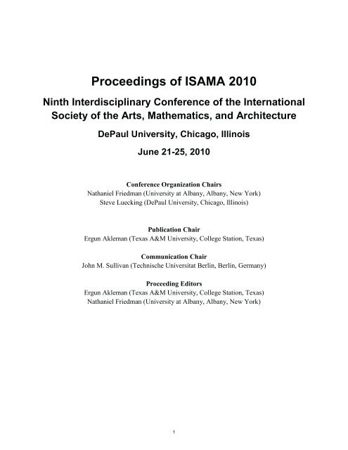
<strong>Proceedings</strong> <strong>of</strong> <strong>ISAMA</strong> <strong>2010</strong><br />
Ninth Interdisciplinary Conference <strong>of</strong> <strong>the</strong> <strong>International</strong><br />
<strong>Society</strong> <strong>of</strong> <strong>the</strong> <strong>Arts</strong>, Ma<strong>the</strong>matics, and Architecture<br />
DePaul University, Chicago, Illinois<br />
June 21-25, <strong>2010</strong><br />
Conference Organization Chairs<br />
Nathaniel Friedman (University at Albany, Albany, New York)<br />
Steve Luecking (DePaul University, Chicago, Illinois)<br />
Publication Chair<br />
Ergun Akleman (Texas A&M University, College Station, Texas)<br />
Communication Chair<br />
John M. Sullivan (Technische Universitat Berlin, Berlin, Germany)<br />
Proceeding Editors<br />
Ergun Akleman (Texas A&M University, College Station, Texas)<br />
Nathaniel Friedman (University at Albany, Albany, New York)<br />
1
Preface<br />
It is a pleasure to return to my hometown Chicago, where Steve Luecking previously hosted a<br />
very successful <strong>ISAMA</strong> 2004 at DePaul University. I wish to express my deep appreciation to<br />
Steve and DePaul once again <strong>for</strong> graciously hosting <strong>ISAMA</strong> <strong>2010</strong>. Since 2004, Millenium Park<br />
has been completed with <strong>the</strong> Frank Gehry Pritzker Pavillion Concert Hall, <strong>the</strong> Anish Kapoor<br />
sculpture Cloud Gate, and <strong>the</strong> Renzo Piano Modern Wing addition to <strong>the</strong> Art Institute <strong>of</strong><br />
Chicago, all very impressive sites within easy walking distance <strong>of</strong> DePaul.<br />
This is <strong>the</strong> ninth <strong>ISAMA</strong> conference since <strong>the</strong> founding <strong>of</strong> <strong>ISAMA</strong> in 1998. Looking back over<br />
<strong>the</strong> years, I have to thank all <strong>the</strong> people that helped co-organize conferences, in particular Carlo<br />
Sequin, Javier Barrallo, Dietmar Guderian, John Sullivan, Jose Martinez-Aroza, Juan Antonio<br />
Maldonado, Reza Sarhangi, Steve Luecking, Ergun Akleman, Vinod Srinivasan, Alfred Peris,<br />
and Joan Peiro. I especially want to thank John Sullivan and Ergun Akleman <strong>for</strong> all <strong>the</strong>ir work in<br />
making our publication Hyperseeing a success. The art/math movement has now been<br />
recognized by <strong>the</strong> MAA = Ma<strong>the</strong>matical Association <strong>of</strong> America and <strong>the</strong> AMS = American<br />
Ma<strong>the</strong>matical <strong>Society</strong>. I want to thank Robert Fathauer <strong>for</strong> organizing <strong>the</strong> many exhibits at <strong>the</strong><br />
joint math meetings <strong>of</strong> <strong>the</strong> MAA and AMS, as well as <strong>the</strong> exhibits at <strong>the</strong> Bridges Conferences,<br />
which have produced a first-class series <strong>of</strong> <strong>Proceedings</strong> due to <strong>the</strong> many years <strong>of</strong> work <strong>of</strong> Reza<br />
Sarhangi, as well as Carlo Sequin, George Hart and Craig Kaplan.<br />
There are also <strong>the</strong> Math and Design conferences organized by Vera Spinadel, <strong>the</strong> Nexus<br />
conferences relating ma<strong>the</strong>matics and architecture and <strong>the</strong> Nexus Network Journal organized and<br />
edited by Kim Williams, and <strong>the</strong> various Hungarian Symmetry Conferences organized by our<br />
friends in Budapest. Most <strong>of</strong> all, thank you so much to all <strong>the</strong> conference participants over <strong>the</strong><br />
years. You made <strong>the</strong> conferences.<br />
Nat Friedman<br />
<strong>ISAMA</strong> <strong>2010</strong> Organizing Committee<br />
Ergun Akleman (Texas A&M University, College Station, Texas, USA)<br />
Javier Barrallo (The University <strong>of</strong> <strong>the</strong> Basque Country, San Sebastian, Spain)<br />
Nathaniel Friedman(University at Albany, Albany, New York, USA)<br />
Stephen Luecking (DePaul University, Chicago, Illinois, USA)<br />
John Sullivan (Technische Universitat Berlin, Berlin, Germany)<br />
3
Contents<br />
No Author(s) Title Pages<br />
1 Douglas Dunham Creating Repeating Patterns with Color Symmetry 7-14<br />
2 Nat Friedman Geometric Sculptures Based on an Angle Iron Module 15-20<br />
3 Mehrdad Garousi and Saied Haghighi Ma<strong>the</strong>matical Trays 21-23<br />
4 Mehrdad Garousi and Saied Haghighi Ma<strong>the</strong>matics and Postmodernism 25-30<br />
5 Gary R. Greenfield Bio-Op Art 31-38<br />
6 Ann Hanson Origami Quilts Workshop 39-40<br />
7 Margaret Lanterman Cut Line and Shape in a Structured Field: A Practical<br />
Introduction to Form and Composition<br />
41-44<br />
8 Guan-Ze Liao A Preliminary Exploration <strong>of</strong> Algorithmic Art: Chaotic<br />
Recursive Motions<br />
9 Yen-Lin Chen, Ergun Akleman, Jianer<br />
Chen and Qing Xing<br />
45-52<br />
Designing Biaxial TextileWeaving Patterns 53-62<br />
10 Donna Lish Dimensions in Crochet 63-67<br />
11 Donna Lish Dimensions in Crochet - Workshop 68-68<br />
12 Yang Liu and Godfried Toussaint A Unique Venetian Meander Pattern in <strong>the</strong> Palazzo Cavalli<br />
Franchetti: A Comparative Geometric Analysis and<br />
Application to Pattern Design<br />
13 Stephen Luecking Constructing and Tiling Hypar Kites 83-90<br />
69-82<br />
14 Stephen Luecking Zoomorphs: Hyparhedral and Taut Skin Surfaces in<br />
Sculpture<br />
15 James Mai From Perception To Cognition And Back Again: An<br />
Overview <strong>of</strong> <strong>the</strong> Paintings <strong>of</strong> James Mai<br />
91-102<br />
103-110<br />
16 James Mallos Triangle-Strip Knitting 111-116<br />
17 Susan McBurney Sullivan and Wright 117-120<br />
18 John McDonald On Beetles, Birds and Butterflies: Non-Linear Barrier<br />
Dynamics<br />
121-128<br />
19 Douglas Peden Polar GridField Geometry 129-136<br />
20 David H. Press String Sculpture – New Work 137-146<br />
21 Robert M. Spann Where Do <strong>the</strong> Repelled Points Go? Visualizing Completely<br />
Chaotic Rational Functions<br />
147-154<br />
22 Elizabeth Whiteley Curved Plane Sculpture: Triangles 155-160<br />
23 Daniel Wyllie Lacerda Rodrigues Ornamental Tilings with Polyflaptiles 161-171<br />
24 Qing Xing and Ergun Akleman Creating Abstract Paintings with Functional Interpolation 173- 181<br />
Papers are ordered according to last name <strong>of</strong> <strong>the</strong> first authors.<br />
5
Creating Repeating Patterns with Color Symmetry<br />
Douglas Dunham<br />
Department <strong>of</strong> Computer Science<br />
University <strong>of</strong> Minnesota, Duluth<br />
Duluth, MN 55812-3036, USA<br />
E-mail: ddunham@d.umn.edu<br />
Web Site: http://www.d.umn.edu/˜ddunham/<br />
Abstract<br />
M.C. Escher’s repeating patterns have two distinguishing features: <strong>the</strong>y interlock without gaps or overlaps, and <strong>the</strong>y<br />
are colored in a regular way. In this paper we will discuss this second characteristic, which is usually called color<br />
symmetry. We will first discuss <strong>the</strong> history and <strong>the</strong>ory <strong>of</strong> color symmetry, <strong>the</strong>n show several patterns that exhibit<br />
color symmetry.<br />
Introduction<br />
Figure 1 below shows a pattern with color symmetry in <strong>the</strong> style <strong>of</strong> <strong>the</strong> Dutch artist M.C. Escher’s “Circle<br />
Limit” patterns. Escher was a pioneer in creating patterns that were colored symmetrically, using two colors<br />
Figure 1: A pattern with 5-color symmetry.<br />
(black-white) and n colors <strong>for</strong> n > 2. In <strong>the</strong> next section, we review <strong>the</strong> history and <strong>the</strong>ory <strong>of</strong> color<br />
symmetry. Then we briefly discuss regular tessellations and hyperbolic geometry, since such tessellations<br />
provide a framework <strong>for</strong> repeating patterns, and hyperbolic geometry allows <strong>for</strong> many different kinds <strong>of</strong><br />
repeating patterns and thus many kinds <strong>of</strong> color symmetry. Next, we explain how to implement color<br />
symmetry in common programming languages. With that background, we show patterns <strong>of</strong> fish like those <strong>of</strong><br />
Figure 1 that illustrate <strong>the</strong>se concepts. Then we discuss Escher’s hyperbolic print Circle Limit III and related<br />
patterns which have an additional color restriction. Finally, we suggest directions <strong>for</strong> future research.<br />
7
Color Symmetry: History and Theory<br />
O<strong>the</strong>rs created patterns with color symmetry be<strong>for</strong>e Escher, but he was quite prolific at making such patterns<br />
and, <strong>the</strong> use <strong>of</strong> color symmetry was one <strong>of</strong> <strong>the</strong> hallmarks <strong>of</strong> his work. As early as 1921 Escher created a<br />
pattern with 2-color (black-white) symmetry shown in Figure 2, 15 years be<strong>for</strong>e <strong>the</strong> <strong>the</strong>ory <strong>of</strong> such patterns<br />
was elucidated [Woods36]. Figure 3 shows a hyperbolic pattern with 2-color symmetry. Starting in <strong>the</strong> mid<br />
Figure 2: An Escher pattern with 2-color symmetry. Figure 3: A hyperbolic pattern <strong>of</strong> angular fish with<br />
2-color symmetry.<br />
1920’s, Escher drew patterns with 3-color symmetry, and in 1938 he created Regular Division Drawing<br />
20 (Figure 6 below, and <strong>the</strong> inspiration <strong>for</strong> Figure 1), a pattern <strong>of</strong> fish, with 4-color symmetry. From<br />
1938 to 1942 Escher developed his own <strong>the</strong>ory <strong>of</strong> repeating patterns, some <strong>of</strong> which had 3-color symmetry<br />
[Schattschneider04]. This was two decades be<strong>for</strong>e ma<strong>the</strong>maticians defined <strong>the</strong>ir own <strong>the</strong>ory <strong>of</strong> n-color<br />
symmetry <strong>for</strong> n > 2 [Van der Waerden61].<br />
In order to understand color symmetry, it is necessary to understand symmetries without respect to color.<br />
A repeating pattern is a pattern made up <strong>of</strong> congruent copies <strong>of</strong> a basic subpattern or motif. A symmetry<br />
<strong>of</strong> a repeating pattern is an isometry (a distance preserving trans<strong>for</strong>mation) that takes <strong>the</strong> pattern onto itself<br />
so that each copy <strong>of</strong> <strong>the</strong> motif is mapped to ano<strong>the</strong>r copy <strong>of</strong> <strong>the</strong> motif. For example, reflection across <strong>the</strong><br />
vertical diameter in Figure 3 is a symmetry <strong>of</strong> that pattern, as are reflections across <strong>the</strong> diameters that make<br />
60 degree angles with <strong>the</strong> vertical diameter. Also rotation by 180 degrees about <strong>the</strong> center is a symmetry<br />
<strong>of</strong> <strong>the</strong> pattern in Figure 2. A color symmetry <strong>of</strong> a pattern <strong>of</strong> colored motifs is a symmetry <strong>of</strong> <strong>the</strong> uncolored<br />
pattern that takes all motifs <strong>of</strong> one color to motifs <strong>of</strong> a single color — that is, it permutes <strong>the</strong> colors <strong>of</strong> <strong>the</strong><br />
motifs. This concept is sometimes called perfect color symmetry. Escher required that colored patterns<br />
adhere to <strong>the</strong> map-coloring principle: motifs that share an edge must be different colors (but motifs <strong>of</strong> <strong>the</strong><br />
same color can share a vertex), and we will follow that principle also. For example, reflection about <strong>the</strong><br />
horizontal or vertical axis through <strong>the</strong> center <strong>of</strong> Figure 2 is almost a color symmetry <strong>of</strong> that pattern since<br />
it interchanges black and white (<strong>the</strong>re are a few small pieces that do not quite correspond). In Figure 1, a<br />
counter-clockwise rotation about <strong>the</strong> center by 72 degrees is a color symmetry in which red → yellow →<br />
blue → brown → white → red. Black remains fixed since it is used as an outline/detail color. Note that if<br />
a symmetry <strong>of</strong> an uncolored pattern has period k, <strong>the</strong>n <strong>the</strong> period <strong>of</strong> <strong>the</strong> color permutation it induces must<br />
8
divide k. In group <strong>the</strong>ory terms, this means that <strong>the</strong> mapping from symmetries to color permutations is a<br />
homomorphism. So, in Figure 1, since rotation about <strong>the</strong> center by 72 degrees has period 5 (and <strong>the</strong> five<br />
central fish must be different colors by <strong>the</strong> map-coloring principle), <strong>the</strong> color permutation also has period 5<br />
since 5 is a prime. In general any rotation <strong>of</strong> prime period k would induce a color permutation <strong>of</strong> period k.<br />
See [Schwarzenberger84] <strong>for</strong> an account <strong>of</strong> <strong>the</strong> development <strong>of</strong> <strong>the</strong> <strong>the</strong>ory <strong>of</strong> color symmetry.<br />
Regular Tessellations and Hyperbolic Geometry<br />
One important kind <strong>of</strong> repeating pattern is <strong>the</strong> regular tessellation, denoted {p, q}, <strong>of</strong> <strong>the</strong> hyperbolic plane<br />
by regular p-sided polygons meeting q at a vertex. Actually this definition also works <strong>for</strong> <strong>the</strong> sphere and<br />
in <strong>the</strong> Euclidean plane. It is necessary that (p − 2)(q − 2) > 4 to obtain a hyperbolic tessellation. If<br />
(p − 2)(q − 2) = 4, <strong>the</strong> tessellation is Euclidean and <strong>the</strong>re are three possibilities: <strong>the</strong> tessellation by squares<br />
{4, 4}, by regular hexagons {6, 3}, and by equilateral triangles {3, 6}. If (p − 2)(q − 2) < 4, <strong>the</strong> tessellation<br />
is spherical and <strong>the</strong>re are five possibilities, corresponding to <strong>the</strong> five Platonic solids. Escher made extensive<br />
use <strong>of</strong> <strong>the</strong> Euclidean tessellations as a framework <strong>for</strong> his Regular Division Drawings [Schattschneider04].<br />
He used {6, 4} in his construction <strong>of</strong> his hyperbolic patterns Circle Limit I and Circle Limit IV; he used<br />
{8, 3} <strong>for</strong> Circle Limit II and Circle Limit III. Figure 4 shows {6, 4} in red superimposed on Circle Limit I;<br />
Figure 5 shows {8, 3} in blue superimposed on Circle Limit II. Figures 1 and 3 are based on <strong>the</strong> tessellations<br />
Figure 4: The {6, 4} tessellation (red) superimposed<br />
on <strong>the</strong> Circle Limit I pattern.<br />
Figure 5: The {8, 3} tessellation (blue) superimposed<br />
on <strong>the</strong> Circle Limit II pattern.<br />
{5, 4} and {6, 6} respectively.<br />
Since <strong>the</strong>re are infinitely many solutions to <strong>the</strong> inequality (p − 2)(q − 2) > 4, <strong>the</strong>re are infinitely many<br />
different hyperbolic patterns. Escher undoubtedly would have created many more such patterns if it had not<br />
required so much tedious hand work. In this age <strong>of</strong> computers, this is not a problem, so we can investigate<br />
many such patterns with many kinds <strong>of</strong> color symmetry.<br />
The patterns <strong>of</strong> Figures 1, 3, 4, and 5 are drawn in <strong>the</strong> Euclidean plane, but <strong>the</strong>y could also be interpreted<br />
as repeating patterns in <strong>the</strong> Poincaré disk model <strong>of</strong> hyperbolic geometry. In this model, hyperbolic points<br />
in this model are just <strong>the</strong> (Euclidean) points within a Euclidean bounding circle. Hyperbolic lines are<br />
represented by circular arcs orthogonal to <strong>the</strong> bounding circle (including diameters). Thus, <strong>the</strong> backbone<br />
9
lines <strong>of</strong> <strong>the</strong> fish lie along hyperbolic lines in Figure 3, as do <strong>the</strong> edges <strong>of</strong> {6, 4} in Figure 4. The hyperbolic<br />
measure <strong>of</strong> an angle is <strong>the</strong> same as its Euclidean measure in <strong>the</strong> disk model — we say such a model is<br />
con<strong>for</strong>mal. Equal hyperbolic distances correspond to ever smaller Euclidean distances toward <strong>the</strong> edge <strong>of</strong><br />
<strong>the</strong> disk. Thus, all <strong>the</strong> fish in Figure 1 are hyperbolically <strong>the</strong> same size, as are all <strong>the</strong> fish in Figure 3.<br />
A reflection in a hyperbolic line is an inversion in <strong>the</strong> circular arc representing that line (or just Euclidean<br />
reflection across a diameter). As in Euclidean geometry, any isometry can be built up from at most<br />
three reflections. For example, successive reflections across intersecting lines produces a rotation about <strong>the</strong><br />
intersection point by twice <strong>the</strong> angle between <strong>the</strong> lines in both Euclidean and hyperbolic geometry. This can<br />
best be seen in Figure 3 which has 120 degree rotations about <strong>the</strong> meeting points <strong>of</strong> noses; <strong>the</strong>re are also 90<br />
degree rotations about <strong>the</strong> points where <strong>the</strong> trailing edges <strong>of</strong> fin tips meet. In Figure 1, <strong>the</strong>re are 72 degree<br />
rotations about <strong>the</strong> tails and 90 degree rotations about <strong>the</strong> dorsal fins. For more on hyperbolic geometry see<br />
[Greenberg08].<br />
Implementation <strong>of</strong> Color Symmetry<br />
Symmetries <strong>of</strong> <strong>of</strong> uncolored patterns in both Euclidean and hyperbolic geometry [Dunham86] can be implemented<br />
as matrices in many programming languages. To implement permutations <strong>of</strong> <strong>the</strong> colors, it is<br />
convenient to use integers to represent <strong>the</strong> colors and arrays to represent <strong>the</strong> permutations. The representation<br />
<strong>of</strong> permutations by cycles or matrices seems less useful. In Figure 1, we let 0 ↔ black, 1 ↔ white, 2<br />
↔ red, 3 ↔ yellow, 4 ↔ blue, and 5 ↔ brown. If α is <strong>the</strong> color permutation induced by counter clockwise<br />
rotation about <strong>the</strong> center by 72 degrees,<br />
( )<br />
0 1 2 3 4 5<br />
α =<br />
0 2 3 4 5 1<br />
in two-line notation. This is easily implemented as an array in some common programming languages as:<br />
α[0] = 0, α[1] = 2, α[2] = 3, α[3] = 4, α[4] = 5, α[5] = 1.<br />
It is <strong>the</strong>n easy to multiply permutations α and β to obtain <strong>the</strong>ir product γ as follows:<br />
<strong>for</strong> i ← 0 to nColors - 1<br />
γ[i] = β[α[i]]<br />
It is also easy to obtain <strong>the</strong> inverse <strong>of</strong> a permutations α as follows:<br />
<strong>for</strong> i ← 0 to nColors - 1<br />
α −1 [α[i]] =i<br />
It is useful to “bundle” <strong>the</strong> matrix representing a symmetry with its color permutation as an array into a<br />
single “trans<strong>for</strong>mation” structure (or class in an object oriented language).<br />
Patterns Based on Escher’s Notebook Drawing 20<br />
Escher’s Notebook Drawing 20, Figure 6, seems to be <strong>the</strong> first <strong>of</strong> his repeating patterns with 4-color symmetry.<br />
It is based on <strong>the</strong> Euclidean square tessellation {4, 4}. It requires four colors since <strong>the</strong>re is a meeting<br />
point <strong>of</strong> three fish near <strong>the</strong> fish mouths and thus needs at least 3 colors, and <strong>the</strong> number <strong>of</strong> colors must divide<br />
4. It was <strong>the</strong> inspiration <strong>for</strong> <strong>the</strong> hyperbolic pattern <strong>of</strong> Figure 1, which as noted above requires at least five<br />
colors since it has rotation points <strong>of</strong> prime period five, and as can be seen, five colors suffice. Figure 7 shows<br />
a related pattern with 4-fold rotations at <strong>the</strong> tails and 5-fold rotations at <strong>the</strong> dorsal fins — <strong>the</strong> reverse <strong>of</strong><br />
Figure 1. We present two more patterns in this family. Figure 8 is based on <strong>the</strong> <strong>the</strong> {5, 5} tessellation. In<br />
order to obtain 4-colored pattern as in Escher’s Notebook Drawing 20, it is necessary that four divides p and<br />
q — Figure 9 shows such a pattern <strong>of</strong> distorted fish based on {8, 4}.<br />
10
Figure 6: Escher’s Notebook Drawing 20.<br />
Figure 7: A fish pattern based on <strong>the</strong> {4, 5} tessellation.<br />
Figure 8: A fish pattern based on <strong>the</strong> {5, 5} tessellation.<br />
Figure 9: A pattern <strong>of</strong> distorted fish based on <strong>the</strong><br />
{8, 4} tessellation.<br />
11
The Color Symmetry <strong>of</strong> Circle Limit III and Related Patterns<br />
Escher’s print Circle Limit III is probably his most attractive and intriguing hyperbolic pattern. Figure 10<br />
shows a computer rendition <strong>of</strong> that pattern. Escher wanted to design a pattern in which <strong>the</strong> fish along a<br />
backbone line were all <strong>the</strong> same color. This is nominally an added restriction to obtaining a symmetric<br />
coloring. However in <strong>the</strong> case <strong>of</strong> Circle Limit III, four colors are required anyway. Certainly at least three<br />
colors are required since three fish meet at left rear fin tips. But three colors are not enough to achieve color<br />
symmetry. A contradiction will arise if we assume that we can re-color some <strong>of</strong> <strong>the</strong> fish in Circle Limit III<br />
using only three colors and while maintaining color symmetry. To see this, focus on <strong>the</strong> yellow fish to <strong>the</strong><br />
upper right <strong>of</strong> <strong>the</strong> center <strong>of</strong> <strong>the</strong> circle (with its right fin at <strong>the</strong> center). Red and blue fish meet at its left fin.<br />
There are two possibilities <strong>for</strong> coloring <strong>the</strong> fish that meet its nose: (1) use two colors, with all <strong>the</strong> “nose”<br />
fish colored yellow and all <strong>the</strong> “tail” fish colored red (to preserve <strong>the</strong> coloring <strong>of</strong> <strong>the</strong> fish at <strong>the</strong> yellow fish’s<br />
left fin), or (2) use three colors, with yellow and red fish as in Circle Limit III, and <strong>the</strong> green fish <strong>of</strong> Circle<br />
Limit III being colored blue instead (since yellow, red, and blue are <strong>the</strong> three colors). In both cases <strong>the</strong> color<br />
symmetry requirement would imply that <strong>the</strong>re were at least three different colors <strong>for</strong> <strong>the</strong> four fish around <strong>the</strong><br />
center <strong>of</strong> <strong>the</strong> circle. In case (1), <strong>the</strong> green lower right fish <strong>of</strong> <strong>the</strong> four center fish would be red instead since<br />
it is a “tail” fish at <strong>the</strong> nose <strong>of</strong> <strong>the</strong> yellow “focus” fish, and <strong>the</strong> upper left fish <strong>of</strong> <strong>the</strong> four center fish would<br />
be blue, since <strong>the</strong> “nose” fishes at <strong>the</strong> tail <strong>of</strong> <strong>the</strong> “focus” fish are blue. In case (2), <strong>the</strong> only way that we can<br />
use three colors is to have fish along <strong>the</strong> same backbone line be <strong>the</strong> same color. In this case <strong>the</strong> green lower<br />
right fish <strong>of</strong> <strong>the</strong> four center would have to be blue, and <strong>the</strong> upper left fish <strong>of</strong> <strong>the</strong> four center fish would be<br />
red. So in both cases <strong>the</strong> central four fish would be colored by at least three different colors, and thus must<br />
use at least four colors to have color symmetry (since <strong>the</strong> center is a 4-fold rotation point), a contradiction<br />
to <strong>the</strong> assumption that Circle Limit III could be 3-colored.<br />
Figure 11 shows a pattern based on <strong>the</strong> {10, 3} tessellation and related to Circle Limit III, but with five<br />
fish meeting at right fins. Like Circle Limit III, Figure 11 also satisfies Escher’s additional restriction that<br />
Figure 10: A computer rendition <strong>of</strong> <strong>the</strong> Circle Limit<br />
III pattern.<br />
Figure 11: A Circle Limit III like pattern based on<br />
<strong>the</strong> {10, 3} tessellation.<br />
fish along <strong>the</strong> same backbone line be <strong>the</strong> same color. Certainly five colors are needed to color this pattern,<br />
12
since <strong>the</strong>re is a 5-fold rotation point in <strong>the</strong> center, but it can be proved that a sixth color, yellow, is actually<br />
needed to satisfy Escher’s restriction.<br />
If Escher’s restriction is removed, it turns out that <strong>the</strong> pattern <strong>of</strong> Figure 11 can be 5-colored, as is shown<br />
in Figure 12. If <strong>the</strong> fish are “symmetric”, with five fish meeting at both <strong>the</strong> right and left fins, <strong>the</strong>n <strong>the</strong> pattern<br />
can be colored with only five colors and still adhere to Escher’s restriction that fish along each backbone<br />
line be <strong>the</strong> same color. Figure 13 shows such a pattern. For more on patterns related to Circle Limit III see<br />
[Dunham09].<br />
Figure 12: A 5-coloring <strong>of</strong> <strong>the</strong> pattern <strong>of</strong> Figure 11.<br />
Figure 13: A 5-colored “symmetric” fish pattern.<br />
Conclusions and Future Work<br />
Except <strong>for</strong> Escher’s patterns, I determined <strong>the</strong> colorings <strong>of</strong> all <strong>the</strong> patterns <strong>of</strong> Figures “by hand”, which was<br />
usually a trial and error process. It seems to be a difficult problem to automate <strong>the</strong> process <strong>of</strong> coloring a<br />
pattern symmetrically — i.e. with color symmetry while adhering to <strong>the</strong> map-coloring principle. And even if<br />
that is possible, it would seem to be even harder if we add Escher’s restriction that fish alone each backbone<br />
line be <strong>the</strong> same color <strong>for</strong> Circle Limit III like patterns.<br />
Acknowledgments<br />
I would like to thank Lisa Fitzpatrick and <strong>the</strong> staff <strong>of</strong> <strong>the</strong> Visualization and Digital Imaging Lab (VDIL) at<br />
<strong>the</strong> University <strong>of</strong> Minnesota Duluth.<br />
References<br />
[Dunham86] D. Dunham, Hyperbolic symmetry, Computers & Ma<strong>the</strong>matics with Applications, Vol. 12B,<br />
Nos. 1/2, 1986, pp. 139–153. Also appears in <strong>the</strong> book Symmetry edited by István Hargittai, Pergamon<br />
Press, New York, 1986. ISBN 0-08-033986-7<br />
[Dunham09] D. Dunham, Trans<strong>for</strong>ming “Circle Limit III” Patterns - First Steps, <strong>Proceedings</strong> <strong>of</strong> <strong>ISAMA</strong> 09,<br />
(eds. Ergun Akleman and Nathaniel Friedman), Albany, New York, pp. 69–73, 2009.<br />
13
[Greenberg08] M. Greenberg, Euclidean & Non-Euclidean Geometry, Development and History, 4th Ed.,<br />
W. H. Freeman, Inc., New York, 2008. ISBN 0-7167-9948-0<br />
[Schattschneider04] D. Schattschneider, M.C. Escher: Visions <strong>of</strong> Symmetry, 2nd Ed., Harry N. Abrams,<br />
Inc., New York, 2004. ISBN 0-8109-4308-5<br />
[Schwarzenberger84] R. L. E. Schwarzenberger, Colour Symmetry, Bulletin <strong>of</strong> <strong>the</strong> London Ma<strong>the</strong>matical<br />
<strong>Society</strong> 16 (1984) 209-240.<br />
[Van der Waerden61] B.L. Van der Waerden and J.J. Burckhardt, Farbgrupen, Zeitschrift für Kristallographie,<br />
115 (1961), pp. 231234.<br />
[Woods36] H.J. Woods, “Counterchange Symmetry in Plane Patterns”, Journal <strong>of</strong> <strong>the</strong> Textile Institute<br />
(Manchester) 27 (1936): T305-T320.<br />
14
Geometric Sculptures Based on an Angle Iron Module<br />
Nat Friedman<br />
artmath@gmail.com<br />
Abstract<br />
A steel angle iron module is used to create a variety <strong>of</strong> geometric sculptures.<br />
Introduction<br />
Several months ago I visited Albany Steel in Albany, NY to inquire about <strong>the</strong> possibility <strong>of</strong> <strong>the</strong> construction <strong>of</strong> a steel<br />
Mobius band. This turned out to require multiple parts which I plan to follow up on later. Meanwhile, I happened to check<br />
out <strong>the</strong> Remainder Room, where all sorts <strong>of</strong> steel cut<strong>of</strong>fs could be bought <strong>for</strong> ½ dollar per pound. In particular, <strong>the</strong>re was a<br />
barrel with about 150 short cut<strong>of</strong>fs <strong>of</strong> angle iron, which is simply two perpendicular rectangles. I started playing with a<br />
few and realized <strong>the</strong>re were probably lots <strong>of</strong> possibilities so I purchased <strong>the</strong>m and took <strong>the</strong>m home. I tried out various<br />
arrangements and this led to <strong>the</strong> steel sculptures discussed below.<br />
Delicate Balance<br />
I first investigated arrangements that were stable due to gravity. A first arrangement consisting <strong>of</strong> two modules is shown<br />
below in Figure 1. Later <strong>the</strong>y were welded toge<strong>the</strong>r.<br />
Figure 1. Two Touching Twice.<br />
Figure 2. Four Touching Twice.<br />
I next realized that I could also use modules and match up corners to construct a raised version <strong>of</strong> Two Touching Twice,<br />
as shown in Figure 2. I had a choice <strong>of</strong> which way to position <strong>the</strong> lower two modules. In Figure 2, <strong>the</strong>y are “facing out” or<br />
“concave out”. They could have been turned around a half turn to face in. I liked <strong>the</strong> positioning in Figure 2 because <strong>the</strong><br />
two lower modules <strong>for</strong>m a little sub-sculpture by <strong>the</strong>mselves with a narrow space between.<br />
15
Two modules touching once are shown raised in Figure 3. The supporting modules are positioned so that <strong>the</strong> concave<br />
sides face each o<strong>the</strong>r. This led to a central arch consisting <strong>of</strong> <strong>the</strong> upper inverted “V” (peak where <strong>the</strong>y touch) and <strong>the</strong>n <strong>the</strong><br />
vertical supporting sides below <strong>the</strong> V.<br />
Figure 3. Two Touching Once in Space.<br />
Figure 4. Three Touching Pairwise.<br />
Three modules touching pairwise are shown Figure 4. This <strong>for</strong>m could also be raised on three supporting modules similar<br />
to Figures 2 or 3. Ano<strong>the</strong>r arrangement <strong>of</strong> three are shown in Figure 5. This <strong>for</strong>m could also be raised up on three more<br />
modules similar to Figures 2 or 3.<br />
Figure 5. Three Touching In Line.<br />
Figure 6. Multidirectional Formation.<br />
The ring <strong>for</strong>mation in Figure 4 can be extended to a ring <strong>of</strong> any number approaching a circle. The linear <strong>for</strong>mation in<br />
Figure 5 can also be extended to a line <strong>of</strong> any number. Moreover, one can arrange <strong>for</strong>mations in various multidirectional<br />
ways, as in Figure 6 <strong>for</strong> example.<br />
Welded Sculptures<br />
Two copies <strong>of</strong> <strong>the</strong> sculpture in Figure 1 are shown welded toge<strong>the</strong>r in Figure 7 in a horizontal position. Here <strong>the</strong> lower<br />
points <strong>of</strong> <strong>the</strong> original supporting modules must match up. This sculpture can be thought <strong>of</strong> as a “polyhedron with<br />
windows”.<br />
Two copies <strong>of</strong> <strong>the</strong> sculpture in Figure 3 are shown welded toge<strong>the</strong>r in Figure 8. The lower half is turned upside down so<br />
corners match up with <strong>the</strong> upper half. This sculpture can also be thought <strong>of</strong> as a polyhedron with windows. The sculptures<br />
in Figures 5 and 6 could also be welded to an inverted copy to obtain some different looking sculptures.<br />
16
Figure 7. Four With Corners Touching.<br />
Figure 8. Six with Corners touching.<br />
Figure 9. Two Perpendicular Spaces.<br />
Figure 10. Two Spaces with Rotation.<br />
Towers <strong>of</strong> Spaces<br />
A tower consisting <strong>of</strong> two spaces is shown in Figure 9. Note that each space is <strong>for</strong>med by a pair <strong>of</strong> modules with one<br />
module inverted with respect to <strong>the</strong> o<strong>the</strong>r. Here each pair is welded toge<strong>the</strong>r and stacked with a half turn so that <strong>the</strong><br />
spaces are perpendicular to each o<strong>the</strong>r.<br />
The two spaces are stacked with a rotation different from a half turn in Figure 10.The rotation is determined by placing<br />
<strong>the</strong> front lower right corner <strong>of</strong> <strong>the</strong> upper module on <strong>the</strong> front upper left corner <strong>of</strong> <strong>the</strong> module below. The rear lower right<br />
corner <strong>of</strong> <strong>the</strong> upper module is placed so it is on <strong>the</strong> upper right edge <strong>of</strong> <strong>the</strong> module below.<br />
Because <strong>of</strong> <strong>the</strong> dimensions <strong>of</strong> <strong>the</strong> module, <strong>the</strong> stacked space above does not tip over, although it looks look like it should.<br />
In fact, a stacking <strong>of</strong> any number <strong>of</strong> spaces will be stable, which was not expected. Three stacked spaces are shown in<br />
Figure 11. Here <strong>the</strong> modules are not welded. For a permanent sculpture, each space pair would be welded, as in Figures 9<br />
and 10. The welded pairs could be stacked without welding, as in Figures 9 and 10, so that one could rotate <strong>the</strong> welded<br />
pairs as desired. For permanence, <strong>the</strong> pairs would be welded toge<strong>the</strong>r in <strong>the</strong> stack.<br />
17
An Architectural Sculpture.<br />
The next sculpture in Figure 12 consists <strong>of</strong> five<br />
modules with a space stacked above two <strong>of</strong>fset<br />
separated perpendicular spaces below, with no<br />
welds. This reminded me <strong>of</strong> an architectural<br />
relationship. The opposite side is shown in Figure<br />
13. In a welded version, <strong>the</strong> three modules below<br />
are welded and <strong>the</strong> two modules <strong>for</strong>ming <strong>the</strong> upper<br />
space are welded. However, <strong>for</strong> ease in lifting when<br />
moving when <strong>the</strong> modules are larger and heavier,<br />
<strong>the</strong> upper space is not welded to <strong>the</strong> lower part.<br />
Reclining Forms.<br />
Three modules are shown in Figure 14. First <strong>the</strong><br />
center module was positioned resting on <strong>the</strong> left<br />
module and <strong>the</strong>n <strong>the</strong> right module was positioned<br />
resting on <strong>the</strong> center module. Welding is not<br />
necessary although <strong>the</strong> modules in Figure 14 are<br />
welded. Since <strong>the</strong> modules are resting on each<br />
o<strong>the</strong>r, I refer to <strong>the</strong> sculpture as a reclining <strong>for</strong>m (<br />
having Henry Moore’s reclining figures in mind).<br />
Ano<strong>the</strong>r welded reclining <strong>for</strong>m is shown in Figure<br />
15. Here <strong>the</strong> left <strong>for</strong>m in Figure 14 is reversed so<br />
that <strong>the</strong> left and center <strong>for</strong>ms are welded along <strong>the</strong><br />
corresponding center edges.<br />
Figure 11. Three Spaces with Rotation.<br />
modules also <strong>for</strong>m a balanced stable sculpture.<br />
In a moment <strong>of</strong> inspiration, I added a fourth module<br />
on <strong>the</strong> right module in Figure 15, as shown in<br />
Figure 16. We note that <strong>the</strong> left module in Figure<br />
16 is not needed <strong>for</strong> stability, as <strong>the</strong> right three<br />
Off Set Forms.<br />
It came as a surprise that <strong>the</strong> middle two modules are also stable by <strong>the</strong>mselves. In fact <strong>the</strong>y can balance thyemselves<br />
without welding. However, this depends on <strong>the</strong> dimensions <strong>of</strong> <strong>the</strong> module. If <strong>the</strong> module is relatively long, <strong>the</strong>n even<br />
welding two toge<strong>the</strong>r edges to edges as <strong>the</strong> middle two in Figure 16, <strong>the</strong> welded two would tip over on <strong>the</strong> left.<br />
Moreover, if <strong>the</strong> middle two are <strong>of</strong>fset and welded, <strong>the</strong>y are still stable in <strong>the</strong> diagonal position, as in <strong>the</strong> case <strong>of</strong> <strong>the</strong> two<br />
modules in Figure 17. An end view is shown in Figure 18.<br />
In Figure 17, it looks like <strong>the</strong> sculpture should tip over. In fact, if <strong>the</strong> two modules are too <strong>of</strong>fset, i.e. too close to each<br />
o<strong>the</strong>r so <strong>the</strong> center space between <strong>the</strong>m is small, <strong>the</strong>n <strong>the</strong>y will tip over to <strong>the</strong> left and <strong>for</strong>ward in Figure 18. Thus Two<br />
Offset is a sculpture that can appear “impossibly stable” when <strong>the</strong> configuration is nearly too <strong>of</strong>fset. We note again that<br />
any possible stability depends on <strong>the</strong> module being relatively short to begin with. Luckily <strong>the</strong> original modules in <strong>the</strong><br />
barrel were relatively short or I wouldn’t have found Two Offset.<br />
18
In Figure 19 we have a version <strong>of</strong> Two Offset with a third module welded above. A front view is shown in Figure 20. I<br />
have also done larger versions <strong>of</strong> <strong>the</strong> right three in Figure 16, which has no <strong>of</strong>fset and has a symmetric front view.<br />
Figure 12. Architectural Sculpture, Five Modules.<br />
Figure 13. Architectural Sculpture, opposite view.<br />
Figure 14. Three Piece Reclining Form 1. Figure 15. Three Piece Reclining Form 2.<br />
Figure 16. Four Piece Reclining Form.<br />
Figure 17. Two Offset.<br />
19
Additional Joinings<br />
A welded join <strong>of</strong> edge to surface occurs in <strong>the</strong> sculpture in Figure 21. A welded join <strong>of</strong> edge to edge occurs <strong>for</strong> <strong>the</strong> left<br />
three modules in Figure 22 with an edge to surface join on <strong>the</strong> right. The last sculpture shown in Figure 23 uses edge to<br />
surface joinings. In conclusion, <strong>the</strong>re still remain more combinations to investigate.<br />
Figure 18. Two Offset, end view.<br />
Figure 19. Offset Three.<br />
Figure 20. Offset Three, front view.<br />
Figure 21. Three Edge to Surface.<br />
Figure 22. Four Edge to Edge and Edge to Surface.<br />
Figure 23. Offset with Edge to Surface.<br />
20
Ma<strong>the</strong>matical Trays<br />
Mehrdad Garousi<br />
Freelance fractal artist, painter and photographer<br />
No. 153, Second floor, Block #14<br />
Maskan Apartments, Kashani Ave<br />
Hamadan, Iran<br />
E-mail: mehrdad_fractal@yahoo.com<br />
http://mehrdadart.deviantart.com<br />
Saied Haghighi<br />
Azad Islamic University, Hamadan Branch<br />
Hamadan, Iran<br />
Email: hagigi_saied@yahoo.com<br />
Abstract<br />
The concept <strong>of</strong> a Seifert surface in knot <strong>the</strong>ory is embellished to obtain designs <strong>for</strong> practical serving trays<br />
with one or more levels.<br />
Introduction<br />
Just like many o<strong>the</strong>r practitioners in <strong>the</strong> interdisciplinary field <strong>of</strong> art and ma<strong>the</strong>matics, our focus is on<br />
designing abstract ma<strong>the</strong>matical models from an aes<strong>the</strong>tic viewpoint. Generally our works are decorative<br />
but do not have a practical application. However, in this article we are concerned with designing practical<br />
serving trays. The motivation <strong>of</strong> <strong>the</strong> design is from knot <strong>the</strong>ory, where we embellish <strong>the</strong> concept <strong>of</strong> a<br />
Seifert surface. Briefly, given a knot, a Seifert surface <strong>for</strong> <strong>the</strong> knot is a two-sided surface having <strong>the</strong> knot<br />
as boundary. A Seifert surface consists <strong>of</strong> disks connected by twisted bands. The motivation is to consider<br />
<strong>the</strong> disks as trays and <strong>the</strong> bands as handles connecting <strong>the</strong> trays. We embellish <strong>the</strong> idea by also<br />
considering knotting <strong>the</strong> bands and varying <strong>the</strong>ir width. The results shown in Figures 1-5 below <strong>of</strong>fer new<br />
<strong>for</strong>ms <strong>for</strong> practical serving trays.<br />
The designs are carried out in a 3D fractal s<strong>of</strong>tware “Incendia” [1]. But, <strong>the</strong> designs are all done in <strong>the</strong><br />
first iteration and without any fractal property. They have only exploited <strong>the</strong> s<strong>of</strong>tware’s abilities in<br />
modeling interesting symmetric 3D <strong>for</strong>ms. Trays due to <strong>the</strong>ir uncommon designs have several areas<br />
which can be used as handles. Handles being intertwined with each o<strong>the</strong>r, have connected <strong>the</strong> main flat<br />
levels <strong>of</strong> double-decker trays. All <strong>of</strong> <strong>the</strong>m have one-fold rotational symmetries.<br />
Basically, <strong>the</strong>re are two distinct ideas behind this kind <strong>of</strong> design process, both <strong>of</strong> which lead to somehow<br />
similar results. One way is intersection knotting which starts from a simple rectangle. This rectangular<br />
plane is <strong>the</strong> main layer <strong>of</strong> <strong>the</strong> tray. The only work we need do is to find a way to connect its four vertices.<br />
The easiest way is to plan <strong>the</strong> paths between vertices in a 3D viewport with right angles. Something like<br />
what we do in providing a 3D Hilbert curve. Ano<strong>the</strong>r thing that should not be neglected is <strong>the</strong> symmetry<br />
<strong>of</strong> <strong>the</strong> whole design. Symmetry provides us with more order. The way two vertices are bridged should be<br />
exactly repeated about two o<strong>the</strong>r vertices.<br />
Despite <strong>the</strong> knots and curvatures we can apply to each <strong>of</strong> <strong>the</strong> bridges, <strong>the</strong>y can be interwoven with each<br />
o<strong>the</strong>r to invite more complication. Maintaining <strong>the</strong> symmetry <strong>of</strong> two paths and intertwining <strong>the</strong>m with<br />
each o<strong>the</strong>r simultaneously is <strong>the</strong> most creative part <strong>of</strong> job. To have a more definite symmetry, I have<br />
connected two neighbor vertices in Figures 1, 2. Along <strong>the</strong> path, between vertices, <strong>the</strong> connecting bands<br />
can have different thicknesses. Because I wanted to have a better efficacy in <strong>the</strong> bottom, I thickened <strong>the</strong>m<br />
where <strong>the</strong>y got closer to <strong>the</strong> main rectangle and rounded <strong>the</strong>m where I needed <strong>the</strong>m as handles. This way,<br />
21
it would be more useful and useable in order to carry things like fruit. This idea is named intersection<br />
knotting because it can be assumed that <strong>the</strong>re had not existed any rectangle basically, and everything<br />
comprises a long knot which has intersected itself once.<br />
Figure 1: Tray 1 (<strong>2010</strong>; © Mehrdad Garousi).<br />
Figure 2: Tray 2 (<strong>2010</strong>; © Mehrdad Garousi).<br />
The second way is plane connecting in which we start with two parallel planes. These flat planes can<br />
provide us with two levels <strong>of</strong> a double-decker tray. Both layers would be used efficiently as two distinct<br />
levels or <strong>the</strong> lower one could be just decorative. Vertices <strong>of</strong> two planes must be connected two by two<br />
with bands. So, here, we will have four bridges. They may have more complication in <strong>the</strong>ir paths like<br />
Figure 3 or reach each o<strong>the</strong>r more simply like those in Figures 4, 5. For instance, in Figure 4, initially,<br />
two closer vertices <strong>of</strong> two levels have been connected with <strong>the</strong> shortest possible band, and <strong>the</strong> second<br />
bridge, connecting two o<strong>the</strong>r neighbor vertices, has tied around <strong>the</strong> short band. It has provided a simple<br />
tie.<br />
The main property <strong>of</strong> <strong>the</strong>se kind <strong>of</strong> designs is that <strong>the</strong>y transcend <strong>the</strong> mind <strong>of</strong> <strong>the</strong> users from <strong>the</strong> prevalent<br />
meaning <strong>of</strong> a tray and introduce <strong>the</strong>m to a more creative <strong>for</strong>m which can be used as a tray along with its<br />
innovation and modernity as a work <strong>of</strong> art..<br />
I hope <strong>the</strong>re would exist some modern centers similar to <strong>the</strong> historic Bauhaus <strong>for</strong> presenting designs with<br />
more focus on artistic and ma<strong>the</strong>matical aspects in order to promote <strong>the</strong> societies expectations <strong>of</strong><br />
everyday tools and goods. Nowadays, with respect to computers, artistic-scientific designing has evolved<br />
much and many artists, ma<strong>the</strong>maticians, and scientists have been recently working in this interdisciplinary<br />
area. In <strong>the</strong> future, one can consider ma<strong>the</strong>matical ideas <strong>for</strong> designing chandeliers, pots, plates, spoons,<br />
<strong>for</strong>ks, chairs, beds, tables, coaches, etc.<br />
[1] Perez, R., http://www.incendia.net/ .<br />
References<br />
22
Figure 3: Tray 3 (<strong>2010</strong>; © Mehrdad Garousi).<br />
Figure 4: Tray 4 (<strong>2010</strong>; © Mehrdad Garousi).<br />
Figure 5: Tray 5 (<strong>2010</strong>; © Mehrdad Garousi).<br />
23
Ma<strong>the</strong>matics and Postmodernism<br />
Saied Haghighi<br />
Azad Islamic University,<br />
Hamadan Branch<br />
Hamadan, Iran<br />
Email: hagigi_saied@yahoo.com<br />
Mehrdad Garousi<br />
Freelance fractal artist, painter and photographer<br />
No. 153, Second floor, Block #14<br />
Maskan Apartments, Kashani Ave<br />
Hamadan, Iran<br />
E-mail: mehrdad_fractal@yahoo.com<br />
http://mehrdadart.deviantart.com<br />
“The artist and <strong>the</strong> scientist each substitute a self-created world <strong>for</strong> <strong>the</strong> experiential one, with <strong>the</strong> goal <strong>of</strong> transcendence.”<br />
(Albert Einstein)[1]<br />
Abstract<br />
This paper with an example aims to show how juxtaposition <strong>of</strong> ma<strong>the</strong>matics, art and <strong>the</strong> new technology <strong>of</strong> computers<br />
launch a new path <strong>of</strong> art creation in postmodernism that results in a new kind <strong>of</strong> aes<strong>the</strong>tics arising from simultaneous<br />
existence <strong>of</strong> order, disorder and complexity.<br />
Keywords: Ma<strong>the</strong>matics, art, 3D sculpting, aes<strong>the</strong>tics<br />
Introduction<br />
Be<strong>for</strong>e <strong>the</strong> second half <strong>of</strong> <strong>the</strong> twentieth century, <strong>the</strong> creation <strong>of</strong> ma<strong>the</strong>matical art did not involve<br />
computers. Most things, from <strong>the</strong> abilities <strong>of</strong> <strong>the</strong> artists to <strong>the</strong> equipment available to <strong>the</strong>m were quite<br />
different. The most important differences rose from <strong>the</strong> process <strong>of</strong> <strong>the</strong> creation <strong>of</strong> ma<strong>the</strong>matical art in<br />
<strong>the</strong>se two eras. Previously, artists interested in new ma<strong>the</strong>matics or ma<strong>the</strong>maticians with artistic and<br />
aes<strong>the</strong>tical desires, created art by constructing ma<strong>the</strong>matical <strong>for</strong>ms or patterns. The creator had to have<br />
particular expertise in ma<strong>the</strong>matics to reach new aes<strong>the</strong>tic <strong>for</strong>ms.<br />
Figure 1. Orange and … (2009; © Mehrdad Garousi).<br />
25
After <strong>the</strong> emergence <strong>of</strong> computers, <strong>the</strong> path <strong>of</strong> ma<strong>the</strong>matical art had a huge change and evolution.<br />
Computers were used to aid <strong>the</strong> artists or even generate artistically ma<strong>the</strong>matical pieces. They<br />
provided a comprehensive field that one could not even imagine be<strong>for</strong>e throughout <strong>the</strong> history <strong>of</strong> <strong>the</strong><br />
ma<strong>the</strong>matics or <strong>the</strong> arts. Computers can do calculations in a moment that might take <strong>the</strong> naked mind<br />
days, weeks or even years. So, <strong>the</strong> field <strong>of</strong> creating modern <strong>for</strong>ms entered a new area full <strong>of</strong><br />
complexities. Be<strong>for</strong>e this, artists were only able to use simple elements <strong>of</strong> ma<strong>the</strong>matics to create<br />
interesting patterns, but today <strong>the</strong>y can use <strong>the</strong> most complicated calculations and figures<br />
simultaneously to create art works.<br />
Renaissance biographer Giorgio Vasari tells us that <strong>the</strong> Florentine architect Filippo Brunelleschi<br />
(1337–1446) took up painting to apply his newly developed <strong>the</strong>ory <strong>of</strong> perspective, based upon Greek<br />
geometry. Additionally, o<strong>the</strong>r major Renaissance painters including Piero della Francesca, Albrecht<br />
Dürer, and Leonardo da Vinci not only experimented and applied principles <strong>of</strong> geometry in <strong>the</strong>ir<br />
work, but published treatises on ma<strong>the</strong>matics. Dürer even developed several drawing machines that<br />
could be used to teach perspective. Especially during <strong>the</strong> European Renaissance, <strong>the</strong> division<br />
separating art and science blurred to <strong>the</strong> point that many <strong>of</strong> its greatest practitioners made nearly equal<br />
contributions to each [2].<br />
It is clearly evident that <strong>the</strong> complexity and <strong>the</strong> novelty <strong>of</strong> <strong>the</strong> ma<strong>the</strong>matical phenomena, appearing in<br />
<strong>the</strong> piece, are <strong>the</strong> main leading elements <strong>of</strong> its beauty. So, <strong>of</strong>ten one <strong>of</strong> <strong>the</strong> most important ways to<br />
attract <strong>the</strong> admirations was to reach a huge amount <strong>of</strong> order in a complex area, like <strong>the</strong> interesting and<br />
accurate tiling <strong>of</strong> Islamic architecture, or to depict some unimaginably spectacular views <strong>of</strong> new<br />
ma<strong>the</strong>matical properties, like those <strong>of</strong> M. C. Escher’s ma<strong>the</strong>matical-artistic works, or finally to show<br />
some geometric results drawn on paper which were impossible and paradoxical in real world, like<br />
impossible figures <strong>of</strong> Oscar Reutersvard. The creator had to start from an initial vision <strong>of</strong> <strong>the</strong><br />
imagined work <strong>of</strong> art in his mind and try to develop it to something interesting and per<strong>for</strong>mable and<br />
finally, after different experimental trials, start to provide <strong>the</strong> final version <strong>of</strong> <strong>the</strong> perfect idea as a<br />
work <strong>of</strong> art. However, sometimes <strong>the</strong> process <strong>of</strong> creation might take a very long time to be per<strong>for</strong>med<br />
and sometimes it would never be done. In fact, <strong>the</strong>re was an imagined or designed ma<strong>the</strong>matical<br />
thought and fantastic amounts <strong>of</strong> experiments and models to construct <strong>the</strong> final work.<br />
Figure 2. Constructive elements <strong>of</strong> “Fire, Water, Soil, and Air” are aligned separately to be compared<br />
without difficulty. It is definite that <strong>the</strong> left halves <strong>of</strong> all <strong>of</strong> <strong>the</strong>m are mirrors to one ano<strong>the</strong>r.<br />
The creation <strong>of</strong> computers and development <strong>of</strong> digital facilities and equipment strongly changed<br />
human’s intuition and insight toward art and aes<strong>the</strong>tics. The very important change is in <strong>the</strong> direction<br />
26
<strong>of</strong> <strong>the</strong> path through which ma<strong>the</strong>matics leads to art. The experimental way <strong>of</strong> <strong>the</strong> past has been getting<br />
reversed recently. Nowadays, <strong>the</strong> least in<strong>for</strong>mation about ma<strong>the</strong>matics could be enough to grasp some<br />
<strong>of</strong> <strong>the</strong> most complex figures one can imagine ma<strong>the</strong>matically. Instead <strong>of</strong> thinking <strong>of</strong> different aspects<br />
and stages <strong>of</strong> reaching <strong>the</strong> required final model, no one can directly run a fractal <strong>for</strong>mula as thousands<br />
<strong>of</strong> lines <strong>of</strong> parameters in a personal computer.<br />
Artists try to explore and find what <strong>the</strong>y want or might seem <strong>of</strong> interest to <strong>the</strong>m straight<strong>for</strong>wardly,<br />
instead <strong>of</strong> following a step by step plot starting in mind and transmitting onto <strong>the</strong> paper. In this order,<br />
different s<strong>of</strong>tware with multiple tools and possibilities play <strong>the</strong> central role. They play an important<br />
role in <strong>the</strong> creation <strong>of</strong> artistic works. They per<strong>for</strong>m like a world which can provide every possibility in<br />
seconds and it can be easily determined if <strong>the</strong>y might be wrong or successful finally. They rescue <strong>the</strong><br />
artist from bunches <strong>of</strong> complex calculations and play a role as a very large and capable potential part<br />
<strong>of</strong> <strong>the</strong> creator’s mind. Creativity only rises from <strong>the</strong> mind <strong>of</strong> <strong>the</strong> artist. However, to grasp it he does<br />
not have to instruct everything from <strong>the</strong> first break, but he must choose <strong>the</strong> area in which he tends to<br />
work and try different facilities and situations according to his needs and knowledge.<br />
TopMod [3] is one <strong>of</strong> several types <strong>of</strong> s<strong>of</strong>tware <strong>for</strong> constructing 3D topological sculptures. It has a<br />
group <strong>of</strong> basic topological polyhedrons and a bunch <strong>of</strong> very useful tools that can be easily applied to<br />
obtain different changes in shapes.<br />
Actually, TopMod does not act only as a tool but as a powerful interactive medium which executes<br />
orders and <strong>of</strong>fers new possibilities to <strong>the</strong> artist. It is <strong>the</strong> artist who starts <strong>the</strong> process <strong>of</strong> creating a work<br />
but after just some simple processes he sees a large number <strong>of</strong> possibilities which were not<br />
anticipated. There<strong>for</strong>e, <strong>the</strong> creator enters new paths and continues this way to develop a satisfying<br />
<strong>for</strong>m and <strong>the</strong>n starts adjusting it by manipulating or smoothing as <strong>the</strong> ultimate stage [4]. The<br />
consequences <strong>of</strong> <strong>the</strong>se processes are ordered and <strong>of</strong>ten symmetric shapes comprising repetitive similar<br />
or semi-similar constituents. However, each <strong>of</strong> <strong>the</strong>se constructive parts is usually quite bizarre. A<br />
good example is <strong>the</strong> work Orange and … (Figure 1). This sculpture, which belongs a family <strong>of</strong><br />
sculptural <strong>for</strong>ms that are introduced in [9,10], is complex 3D shape involves a six-arm shape, each <strong>of</strong><br />
<strong>the</strong> arms completely similar and <strong>the</strong> whole shape somehow symmetric. The 3D shape is made up <strong>of</strong><br />
four distinct constituents none <strong>of</strong> which ever touch <strong>the</strong> o<strong>the</strong>rs.<br />
In Figure 2, I have broken <strong>the</strong> unification <strong>of</strong> <strong>the</strong> sculpture and have arranged all four constituents in a<br />
line with different colors to have a better distinction. You can see that blue and pink ones are exactly<br />
similar and so are green and yellow ones. The most important subject is <strong>the</strong> <strong>for</strong>m <strong>of</strong> each <strong>of</strong> <strong>the</strong><br />
components. They have odd and unexpected identities. It is here that one understands how order and<br />
disorder could integrate in one whole and entity.<br />
Figure 3. Pink and blue bands placed<br />
in <strong>the</strong>ir original positions provide a<br />
one-fold rotational symmetry in spite<br />
<strong>of</strong> <strong>the</strong>ir own asymmetry.<br />
Figure 4. Yellow and green bands<br />
have a same behaviour in <strong>the</strong>ir ally.<br />
Figure 5. All four bands have been<br />
placed accurately to be interwoven<br />
without any failure.<br />
27
Organic <strong>for</strong>m like <strong>the</strong> beauty simultaneously exhibits balance and <strong>the</strong> lack <strong>of</strong> it, homeostasis and<br />
homeorhesis. Homeostasis is a balanced wholeness, integrity, and self regulation. Homeorhesis is a<br />
fluid structure <strong>of</strong> growth, trans<strong>for</strong>mation, and evolution [5].<br />
Now, we start to inquire how <strong>the</strong>se amorphous asymmetric <strong>for</strong>ms begin to construct such an ordered<br />
unity. In Figure 3 we can see <strong>the</strong> arrangement <strong>of</strong> two similar blue and pink constituents. As it is clear<br />
from <strong>the</strong> upside view point, <strong>the</strong>y are founding some kind <strong>of</strong> one-fold rotational symmetry that invites<br />
order into <strong>the</strong>ir ally. This is similarly true about <strong>the</strong> position <strong>of</strong> <strong>the</strong> green and yellow ones in Figure 4<br />
in <strong>the</strong> same way. The upside point <strong>of</strong> view is chosen in order to show <strong>the</strong> symmetry <strong>of</strong> <strong>the</strong><br />
combinations more clearly.<br />
Figure 6. Starting with <strong>the</strong> creation process by adding one handle.<br />
Figure 7. Adding six handles.<br />
At <strong>the</strong> final step, depicted in Figure 5, both dual groups are combined to result in <strong>the</strong> completed<br />
interwoven sculpture. The way <strong>of</strong> convolution <strong>of</strong> <strong>the</strong>se two groups is <strong>the</strong> most accurate part whereby<br />
<strong>the</strong> least amount <strong>of</strong> inaccuracy will appear. The smallest mistake will result in ei<strong>the</strong>r <strong>the</strong> elimination<br />
<strong>of</strong> <strong>the</strong> symmetry or <strong>the</strong> touch <strong>of</strong> <strong>the</strong> bands.<br />
Now, <strong>the</strong> final sculpture, yet ma<strong>the</strong>matically, which has only a one-fold rotational symmetry, due to<br />
<strong>the</strong> very similarity between all its six arms, seems almost symmetric in all directions. In fact, instead<br />
<strong>of</strong> symmetry <strong>the</strong>re is some kind <strong>of</strong> similarity throughout <strong>the</strong> shape.<br />
Creation Process<br />
I am going to show <strong>the</strong> process through which I have constructed <strong>the</strong> piece myself step by step in<br />
TopMod. The creative process starts with a simple dodecahedron (Figure 6(a)). Now we start to make<br />
handles between polygons. TopMod has a nice tool in this regard named Add Handle Mod. I have<br />
connected every two neighbor polygons to each o<strong>the</strong>r with one complete twist <strong>of</strong> <strong>the</strong> handle (Figure<br />
6(b)).<br />
The result <strong>of</strong> all <strong>the</strong>se bridges can be seen in Figure 7. Now we have <strong>the</strong> basic shape <strong>of</strong> our main six<br />
arms built. My settings <strong>for</strong> making handles is shown in <strong>the</strong> Tool Options box opened on <strong>the</strong> up-left <strong>of</strong><br />
<strong>the</strong> viewport in TopMod, depicted in Figure 8. But <strong>the</strong> very essential thing is to determine which<br />
vertices <strong>of</strong> two neighbor polygons are to be connected. In Figure 8 <strong>the</strong>re are five possibilities <strong>for</strong><br />
vertex A to be connected to one <strong>of</strong> <strong>the</strong> vertices <strong>of</strong> polygon b, each <strong>of</strong> which will yield a completely<br />
different result. To obtain our suitable result, we should select <strong>the</strong> coincided vertices. Two neighbor<br />
pentagons have two coincided vertices which can be selected. So, we can connect two pentagons, a<br />
and b, by selecting ei<strong>the</strong>r vertices <strong>of</strong> A and A’, or B and B’ as <strong>the</strong> basis <strong>of</strong> <strong>the</strong> bridge.<br />
Figure 8 shows how to connect two pentagons, a and b, with one twisted handle. We have five<br />
different choices to connect <strong>the</strong>ir vertices. For instance, each vertex <strong>of</strong> polygon b can be connected to<br />
each <strong>of</strong> five vertices <strong>of</strong> polygon a. Having divided all surfaces to smaller components by means <strong>of</strong><br />
Doo Sabin tool, we easily select polygons in distinct loops. These actions are shown in Figure 9(a, b).<br />
28
Figure 9 shows how to choose small polygons as connected loops. TopMod has a useful tool named<br />
“Select Face Loop”. By one click on <strong>the</strong> common edges <strong>of</strong> two polygons, this tool automatically<br />
selects all o<strong>the</strong>r similar polygons aligned with <strong>the</strong>m as open or closed groups.<br />
There is a very handy and useful tool named Ring Modeling Thickness Mode which can engrave<br />
selected loops from inside <strong>the</strong> mesh <strong>the</strong> result <strong>of</strong> which is Figure 10. As a matter <strong>of</strong> fact, <strong>the</strong> magical<br />
ability <strong>of</strong> TopMod per<strong>for</strong>ms here. It engraves <strong>the</strong> central core <strong>of</strong> <strong>the</strong> mesh so artistically and with<br />
special expertise which could not be ever depicted by hand on a two dimensional paper or easily<br />
carved in a real 3D material. By using Doo Sabin two additional times, we will have a smoo<strong>the</strong>r and<br />
more delightful result (Figure 11).<br />
Figure 8. Connecting two polygons a<br />
and b with one twisted handle.<br />
Figure 9. Choosing small polygons as connected loops.<br />
After all <strong>the</strong>se modeling stages in TopMod, I have transmitted <strong>the</strong> result as a raw mesh to Luxology<br />
Modo [6]. Having per<strong>for</strong>med some modifications and defined colors, reflections, lightings, and some<br />
o<strong>the</strong>r details, I rendered <strong>the</strong> ultimate image as my final work <strong>of</strong> art.<br />
In this paper, I did not intend to show how this certain piece was created but to explain <strong>the</strong> process <strong>of</strong><br />
creation <strong>of</strong> most <strong>of</strong> topological 3D sculptures in postmodernism.<br />
Now, my question is how a traditional sculptor might be able to imagine and make such a sculpture?<br />
In traditional art, <strong>the</strong> artist had to imagine <strong>the</strong> final result in his mind and try to find a way to obtain it.<br />
Was it actually possible <strong>for</strong> this artist to imagine a 3D shape like we described here with such<br />
properties? Could he imagine those constructive parts <strong>of</strong> Figure 2 and <strong>for</strong>esee <strong>the</strong> properties <strong>of</strong> <strong>the</strong><br />
<strong>for</strong>m provided by <strong>the</strong>ir unification? This is <strong>the</strong> wonderful ability <strong>of</strong> computer art that makes it possible<br />
to reach shapes completely beyond <strong>the</strong> imagination according to <strong>the</strong>ir complexities. The success <strong>of</strong><br />
this way rises from a main phenomenon that is <strong>the</strong> conversion <strong>of</strong> <strong>the</strong> process <strong>of</strong> making art in<br />
postmodernist ma<strong>the</strong>matical art.<br />
Creation in new media, due to its whole dependence upon ma<strong>the</strong>matics, starts from basic<br />
ma<strong>the</strong>matical shapes like simple polygons or polyhedrons and extends to more complex <strong>for</strong>ms. Thus,<br />
it is not essential to have a complete image <strong>of</strong> <strong>the</strong> final model. One might start with a basic shape and<br />
after minutes or hours <strong>of</strong> playing around with different possibilities and manipulations; obtain an<br />
interesting result which has not been seen be<strong>for</strong>e. Like what first I did about my described sculpture, I<br />
started to play with a pentahedron and by applying my personal techniques, explained above step by<br />
step, attained such a complex shape that was not expected be<strong>for</strong>e. It was I who created it. However, I<br />
did not clearly know what I was approaching.<br />
The creative process doesn’t exist in a vacuum. It’s a highly integrated activity reflecting history,<br />
aes<strong>the</strong>tic <strong>the</strong>ory, and <strong>of</strong>ten <strong>the</strong> technological breakthroughs <strong>of</strong> <strong>the</strong> day. This was certainly <strong>the</strong> case<br />
during <strong>the</strong> Renaissance, when artists, engineers, scientists, and thinkers all came toge<strong>the</strong>r to create<br />
truly remarkable works <strong>of</strong> art and engineering. Over <strong>the</strong> last few decades, we’ve been experiencing<br />
our own Renaissance with <strong>the</strong> proliferation <strong>of</strong> digital technology [7].<br />
29
Conclusion<br />
Postmodern art is about interactive systems ra<strong>the</strong>r than static objects. It appreciates process more than<br />
product. The prototype <strong>for</strong> this postmodern dynamic is <strong>the</strong> process <strong>of</strong> art making itself, <strong>the</strong> creative<br />
process that trans<strong>for</strong>ms mental worlds <strong>of</strong> thoughts and feelings into environmental expressions [5]. In<br />
<strong>the</strong> new era <strong>of</strong> geometrically digital sculpting, ma<strong>the</strong>matics is <strong>the</strong> path through which amazing shapes<br />
can be discovered.<br />
Some sculptors work at physically manifesting structures and ma<strong>the</strong>matical concepts that usually are<br />
difficult to visualize and <strong>of</strong>ten do not occur in nature. The contrast between <strong>the</strong> physicality <strong>of</strong> <strong>the</strong><br />
sculpture and <strong>the</strong> cerebral nature <strong>of</strong> <strong>the</strong> ma<strong>the</strong>matics enhances <strong>the</strong> experience <strong>of</strong> <strong>the</strong> sculptures [8].<br />
The fact <strong>of</strong> <strong>the</strong> matter is that juxtaposition <strong>of</strong> art, ma<strong>the</strong>matics and computer technology has led to an<br />
extensive movement whereby much earlier impossibility can now be possible.<br />
Figure 1. Final Shape.<br />
Figure 11. Smoo<strong>the</strong>d Final Shape.<br />
References<br />
[1] Eistein, A. (1934) Principles <strong>of</strong> Research in A. Einstein, Essays in Science, Philosophical Library, NY.<br />
[2] Greenberg, I. (2007) Processing: Creative Coding and Computational Art, p. 8, Friends <strong>of</strong> ED, USA.<br />
[3] TopMod: Topological Mesh Modeler, Aavailable at http://www.topmod3d.org .<br />
[4] Garousi, M. (2009) TopMod and Creativity, Hyperseeing, fall-winter 2009, available at<br />
http://www.isama.org/hyperseeing/ .<br />
[5] Alexenberg, M. (2006) The Future <strong>of</strong> Art in a Digital Age: From Hellenistic to Hebraic Consciousness, pp.<br />
114, 139, Intellect Ltd, UK.<br />
[6] Luxology Modo, Available at http://www.luxology.com .<br />
[7] Greenberg, I. (2007) Processing: Creative Coding and Computational Art, p. 1, friends <strong>of</strong> ED, USA.<br />
[8] Wilson, S. (2002) In<strong>for</strong>mation <strong>Arts</strong>: Intersections <strong>of</strong> Art, Science, and Technology, pp. 322, MIT Press,<br />
USA.<br />
[9] Akleman E., Srinivasan V. and Chen J. (2003) Interactive Rind Modeling, <strong>Proceedings</strong> <strong>International</strong><br />
Conference on Shape Modeling and Applications, pp. 23-31.<br />
[10] Akleman E., (2006) Symmetric Sculptures, SIGGRAPH and Bridges 2006 Art Exhibits, August.<br />
30
Bio-Op Art<br />
Gary R. Greenfield<br />
Department <strong>of</strong> Ma<strong>the</strong>matics & Computer Science<br />
University <strong>of</strong> Richmond<br />
Richmond, VA 23173, USA<br />
E-mail: ggreenfi@richmond.edu<br />
Abstract<br />
We discuss a series <strong>of</strong> digital biological op art -- Bio-Op Art -- prints which we obtained from visualizations <strong>of</strong> a<br />
simulation <strong>of</strong> cellular morphogenesis. Our simulation models <strong>the</strong> change in concentration within cells over time <strong>of</strong><br />
four syn<strong>the</strong>tic transcription factors. These changes are caused by <strong>the</strong> interactions <strong>of</strong> transcription factors with<br />
artificial genomes. The simulation is complex and difficult to control, <strong>the</strong>re<strong>for</strong>e both <strong>the</strong> genetic material and <strong>the</strong><br />
cell configurations used to obtain <strong>the</strong>se visualizations must be found by exploration and experimentation. There is<br />
an underlying satisfaction knowing that determinism and complexity are <strong>the</strong> basis <strong>for</strong> such dizzying orderliness.<br />
Introduction<br />
Op Art, or optical art, is a style <strong>of</strong> visual art that makes use <strong>of</strong> optical illusions [4][10]. The term Op Art<br />
first appeared in <strong>the</strong> October 1964 issue <strong>of</strong> Time magazine, and <strong>the</strong> subsequent Op Art movement became<br />
enormously popular in <strong>the</strong> sixties. The intent was to make images ``dance’’ by <strong>for</strong>cing <strong>the</strong> eye to<br />
constantly shift focus in order to concentrate on one aspect or <strong>the</strong> o<strong>the</strong>r. Because it relies on line and<br />
pattern to obtain trompe l’oeil effects, Op Art is <strong>of</strong>ten highly geometric and orderly. Perhaps <strong>the</strong> two most<br />
recognizable artists associated with Op Art are Victor Vasarely [9] and Bridget Riley. Artists such as<br />
Josef Albers, Richard Allen, Richard Anuszkiewicz, Carlos Cruz-Diez, and Julian Stanczak are also<br />
frequently mentioned.<br />
In this paper I discuss a series <strong>of</strong> visualizations that I call Bio-Op Art that were inspired by Op Art. More<br />
precisely, I describe how I adapted an image generation technique that I had used previously (see<br />
[5][6][7][8]) <strong>for</strong> various evolutionary art projects to obtain this new series. My technique is based on a<br />
model <strong>of</strong> Eggenberger [3] <strong>for</strong> simulating cellular morphogenesis<br />
Genesis <strong>of</strong> <strong>the</strong> project<br />
I decided to experiment with matrices <strong>of</strong> simulated cells that were highly patterned by making use <strong>of</strong><br />
genetic material that I obtained from a series <strong>of</strong> evolutionary art experiments that were done to test ideas<br />
on how to evolve artificial genomes in complex, difficult to evaluate simulated evolution generative art<br />
systems [8]. After tuning several critical parameters, this led to two Op Art images that were submitted to<br />
<strong>the</strong> juried <strong>2010</strong> Joint Ma<strong>the</strong>matics Meeting Art Exhibition. The web site <strong>for</strong> <strong>the</strong> <strong>2010</strong> JMM exhibition can<br />
be accessed at http://www.bridgesmathart.org/art-exhibits/jmm10/index.html. Figure 1 shows <strong>the</strong> image<br />
that was accepted <strong>for</strong> this JMM exhibition and appears in its catalog [1] and on its web site. The image in<br />
Figure 1 was part <strong>of</strong> a series <strong>of</strong> four images. Thanks to encouragement from a colleague, I continued to<br />
pursue this <strong>the</strong>me after <strong>the</strong> exhibition deadline had passed. My results led to <strong>the</strong> images and techniques I<br />
wish to present here.<br />
31
Figure 1: Gary Greenfield, It’s Not That Simple, I. Digital Print. 10” x 10”, 2009.<br />
The cellular morphogenesis model<br />
My generative scheme is based on simulating cellular morphogenesis. The model I use is due to<br />
Eggenberger [3] but it should be noted that <strong>the</strong>re are now more sophisticated variations [2]. My initial<br />
adaptation <strong>of</strong> Eggenberger’s model to evolutionary art was presented in [5] and [8]. More recent work<br />
involving <strong>the</strong> notion <strong>of</strong> evolutionary refinement is found in [6]. In general, so called “real world’’ biology<br />
simulations are very complicated. Here, in <strong>the</strong> interests <strong>of</strong> focusing on <strong>the</strong> Op Art results, I will only<br />
provide a cursory description. The most comprehensive account <strong>of</strong> my scheme can be found in [7].<br />
An image obtained from my simulation is a visualization <strong>of</strong> a matrix <strong>of</strong> simulated cells. The simulated<br />
cells are initialized with concentrations <strong>of</strong> four syn<strong>the</strong>tic substances that represent transcription factors, or<br />
TFs. The cells are visualized by representing <strong>the</strong>m as blocks <strong>of</strong> pixels, where <strong>the</strong> concentrations <strong>of</strong> three<br />
<strong>of</strong> <strong>the</strong> cell’s four TFs become <strong>the</strong> components <strong>for</strong> <strong>the</strong> pixel’s RGB color. The cell’s remaining colorless<br />
TF plays an important but indirect role. To repeat, <strong>the</strong> scheme is complicated. The basic idea is that <strong>the</strong><br />
concentrations <strong>of</strong> <strong>the</strong> TFs determine which <strong>of</strong> <strong>the</strong> cell’s genes are expressed and that in turn determines<br />
how <strong>the</strong> concentrations <strong>of</strong> <strong>the</strong> TFs change. Simulating each cell’s development requires an update cycle<br />
consisting <strong>of</strong> a gene expression calculation followed by a TF concentration calculation. This update cycle<br />
is per<strong>for</strong>med <strong>for</strong> all cells <strong>for</strong> a fixed number <strong>of</strong> iterations and <strong>the</strong>n <strong>the</strong> visualization is written out to file.<br />
A cell genome consists <strong>of</strong> four gene units. A gene unit consists <strong>of</strong> two regulatory genes and one structural<br />
gene. A gene consists <strong>of</strong> eight digits. With certain exceptions <strong>for</strong> ``marker’’ digits, digits are constrained<br />
to lie in <strong>the</strong> range zero through four. Genes can be parsed to produce an <strong>of</strong>fset, a diffusion coefficient, a<br />
type, or four separate constants. In order to determine whe<strong>the</strong>r a structural gene S within a cell’s gene unit<br />
is currently expressed, or active, one considers <strong>the</strong> j-th regulatory gene R j and begins by using <strong>the</strong><br />
32
egulatory gene’s constants toge<strong>the</strong>r with global constants w i to calculate <strong>the</strong> regulatory gene’s affinity f i<br />
<strong>for</strong> <strong>the</strong> i-th TF. This is a signed quantity. Next, assuming c i is <strong>the</strong> current concentration <strong>of</strong> <strong>the</strong> cell’s i-th<br />
TF, one calculates an activity level r j <strong>for</strong> <strong>the</strong> j-th regulatory gene R j by letting r j = Σ f i c i . Summing over<br />
all regulatory genes we obtain <strong>the</strong> activation measurement a = 1/(1 + exp(Σ r j )). Finally, we threshold this<br />
result to obtain an activity level γ <strong>for</strong> S <strong>of</strong> -1, +1, or 0. For convenience, we say <strong>the</strong> structural gene S is<br />
activated in an excitory state if γ = +1, activated in an inhibitory state if γ = -1, and not activated<br />
o<strong>the</strong>rwise. When activated, <strong>the</strong> concentration <strong>of</strong> <strong>the</strong> TF specified by <strong>the</strong> structural gene's type is increased<br />
(respectively decreased) by a fixed amount. Moreover, if <strong>the</strong> concentration <strong>of</strong> <strong>the</strong> cell’s colorless TF is<br />
above a certain threshold <strong>the</strong>n <strong>the</strong> structural gene’s diffusion coefficient will be used to effect <strong>the</strong><br />
distribution <strong>of</strong> that change over neighboring cells.<br />
Obtaining visualizations<br />
Each image we discuss here requires three different types <strong>of</strong> cells. One <strong>of</strong> <strong>the</strong> cell types is designated as<br />
<strong>the</strong> substrate while <strong>the</strong> o<strong>the</strong>r two types <strong>of</strong> cells are thought <strong>of</strong> as specialized cells. Images are <strong>for</strong>med by<br />
considering a matrix <strong>of</strong> cells where blocks <strong>of</strong> specialized cells are surrounded with substrate cells. The<br />
border cells <strong>of</strong> <strong>the</strong> matrix toge<strong>the</strong>r with all <strong>the</strong> specialized cells in <strong>the</strong> matrix are initialized with trace<br />
level concentrations (0.0003) <strong>of</strong> each <strong>of</strong> <strong>the</strong> four TFs. The update cycle <strong>for</strong> every cell in <strong>the</strong> matrix is<br />
repeated a fixed number <strong>of</strong> times, after which each cell is enlarged to a k x k block <strong>of</strong> pixels that are<br />
colored by interpreting <strong>the</strong> concentrations <strong>of</strong> <strong>the</strong> first three TFs <strong>of</strong> <strong>the</strong> cell as <strong>the</strong> RGB components, The<br />
image in Figure 1 used a 200 x 200 matrix <strong>of</strong> cells, block size k = 10 and iteration count 400. Recall that<br />
each cell genome needs four gene units, and each gene unit needs three genes. To give some indication <strong>of</strong><br />
why it is so difficult to understand (i.e. predict) how <strong>the</strong> concentrations <strong>of</strong> <strong>the</strong> TFs will vary over time,<br />
consider <strong>the</strong> following three cell genomes that were used <strong>for</strong> Figure 1 and that are listed by using one<br />
gene unit per line.<br />
14002031 31230415 40223246<br />
13322342 21331135 13440136<br />
30134332 13102135 11222246<br />
40332114 12320415 43214136<br />
22300210 10302415 40122216<br />
32111010 00233025 43102336<br />
43024104 44010205 20023336<br />
33421020 40003235 21204326<br />
24201444 32340015 41114446<br />
23341110 12132005 24043216<br />
41044041 22134325 10041126<br />
20321013 44102425 43140016<br />
It is no wonder that it is next to impossible to design genomes by hand in such a way that <strong>the</strong> color <strong>of</strong> any<br />
<strong>of</strong> <strong>the</strong> cells in <strong>the</strong> matrix can be pre-determined! To make image size and image resolution more<br />
manageable, <strong>for</strong> <strong>the</strong> remainder <strong>of</strong> this paper we use 100 x 100 matrices <strong>of</strong> cells, block size k = 5, and<br />
iteration counts in <strong>the</strong> range from 50 to 300. Images are reproduced at 150 dpi.<br />
33
Source genetic material<br />
I used three different sets <strong>of</strong> genomes which hence<strong>for</strong>th I will refer to as <strong>the</strong> B, C, and F series genomes,<br />
or data sets. Fur<strong>the</strong>r, <strong>the</strong>re were three variants <strong>of</strong> F which I denoted as F1, F2, and F3. Thus I had a total<br />
<strong>of</strong> five data sets. These five data sets were originally obtained using an exploratory evolutionary search.<br />
This means that three genomes <strong>for</strong> cells were randomly generated, a small matrix <strong>of</strong> cells was seeded with<br />
some <strong>of</strong> <strong>the</strong> specialized cells, and after a fixed number <strong>of</strong> updates <strong>the</strong> result was evaluated based on such<br />
factors as <strong>the</strong> mean and variance <strong>of</strong> TF concentrations, <strong>the</strong> number <strong>of</strong> expressed genes, <strong>the</strong> number <strong>of</strong><br />
non-black cells, etc. In o<strong>the</strong>r words, automated fitness calculations were used to drive a genetic algorithm<br />
which invoked genetic operators to recombine and develop strains <strong>of</strong> cells that showed promising<br />
characteristics [6]. Of course, in <strong>the</strong> final analysis, following several hours <strong>of</strong> computation, I had to<br />
visually inspect <strong>the</strong> few dozen possibilities that had been winnowed out to select <strong>the</strong> five data sets I<br />
actually used.<br />
Bio-Op Art examples<br />
Motivated by Figure 1, <strong>the</strong> basic pattern I chose to experiment with used specialized cells<br />
organized into a regular 20 x 20 grid embedded within a 50 x 50 matrix <strong>of</strong> substrate cells. The<br />
most interesting designs occurred when blocks <strong>of</strong> specialized cells were used alternately in this<br />
scheme. In experimenting with <strong>the</strong> sizes <strong>of</strong> <strong>the</strong> blocks <strong>of</strong> specialized cells, I tried 1 x 1 blocks, 3<br />
x 3 blocks, and alternating 1 x 1 and 3 x 3 blocks. By ``experiment’’ I mean that I tried all five<br />
data sets with all three configurations and inspected <strong>the</strong> results every 50 iterations. Figure 2<br />
shows a 3 x 3 example from <strong>the</strong> C series. Figure 3 shows an alternating 1 x 1 and 3 x 3 example<br />
from <strong>the</strong> C series. Figures 4 and 5 are F2 and F3 series examples respectively.<br />
Figure 2: From <strong>the</strong> C series, after 100 iterations, alternating 3 x 3 blocks <strong>of</strong> specialized cells.<br />
34
Figure 3: From <strong>the</strong> C series, after 150 iterations, alternating 1x1 and 3 x 3 blocks <strong>of</strong> specialized cells.<br />
Figure 4: From <strong>the</strong> F2 series, after 150 iterations, alternating 3 x 3 blocks <strong>of</strong> specialized cells.<br />
35
Figure 5: From <strong>the</strong> F3 series, after 250 iterations, alternating 1 x 1 and 3 x 3 blocks <strong>of</strong> specialized cells.<br />
Variations on a <strong>the</strong>me<br />
I also experimented with using additional sizes <strong>of</strong> blocks <strong>of</strong> alternating cells as an overlay. My first<br />
attempt failed, since <strong>the</strong> larger blocks I introduced did not create optical illusions but ra<strong>the</strong>r resembled<br />
Persian carpet patterns. Figure 6 shows an example from <strong>the</strong> F1 series <strong>of</strong> this phenomenon. I was more<br />
successful when I used alternating sizes in <strong>the</strong> overlay. Figure 7 shows an alternating 5 x 5 and 7 x 7<br />
pattern overlaid on an alternating 1 x 1 and 3 x 3 pattern from <strong>the</strong> F3 series.<br />
Conclusions/reflections<br />
Artistically, I find a sense <strong>of</strong> extreme satisfaction in knowing that overwhelming, mind-numbing<br />
complexity can lead to such regularity and intricacy. Technically, I find an even greater satisfaction in<br />
knowing that only by using algorithms and custom s<strong>of</strong>tware am I able to obtain compositions with color<br />
schemes that I I find unique and appealing. My hope is that a viewer, who knows that a program was<br />
necessary to make <strong>the</strong> image, will be able to draw an analogy between products and underlying processes.<br />
Acknowledgment<br />
I would like to thank Della Fenster <strong>for</strong> her enthusiasm and encouragement which motivated me to search<br />
<strong>for</strong> <strong>the</strong> additional examples shown here.<br />
36
Figure 6: From <strong>the</strong> F1 series, after 150 iterations, alternating 1 x 1 and 3 x 3 blocks <strong>of</strong> specialized cells<br />
with an additional overlay <strong>of</strong> a 3 x 3 grid <strong>of</strong> alternating 7 x7 blocks <strong>of</strong> specialized cells. The illusion is<br />
disrupted and <strong>the</strong> result seems more like a Persian rug.<br />
Figure 7: From <strong>the</strong> F3 series, after 200 iterations, alternating 1 x 1 and 3 x 3 blocks <strong>of</strong><br />
specialized cells overlaid with an alternating 5x5 and 7x7 grid <strong>of</strong> specialized cells.<br />
37
References<br />
[1] Burns, A., and Fathauer, R. (<strong>2010</strong>): <strong>2010</strong> Joint Ma<strong>the</strong>matics Meetings Exhibition <strong>of</strong> Ma<strong>the</strong>matical<br />
Art, Tesselations, Phoenix, AZ.<br />
[2] Chavoya, A., and Du<strong>the</strong>n, Y. (2007): An artificial development model <strong>for</strong> cell pattern generation. In<br />
ACAL '07: <strong>Proceedings</strong> <strong>of</strong> <strong>the</strong> 3rd Australian Conference on Artificial Life, Springer, 61--71.<br />
[3] Eggenberger, P. (1997): Evolving morphologies <strong>of</strong> simulated 3d organisms based on differential gene<br />
expression. In <strong>Proceedings</strong> <strong>of</strong> <strong>the</strong> Fourth European Conference on Artificial Life (ECAL97),<br />
Springer Verlag, 205--213.<br />
[4] Follin, F., Pias, C., and Weinhart, M. (2007): Op Art, Buchhandlung Wal<strong>the</strong>r Konig GmbH & Co<br />
Abt. Verlag, Germany.<br />
[5] Greenfield, G. (2005): Abstract art from a model <strong>for</strong> cellular morphogenesis. In R. Sarhangi and R.<br />
Moody (eds.) BRIDGES 2005 Conference <strong>Proceedings</strong>, 137--142.<br />
[6] Greenfield, G. (<strong>2010</strong>): Generative art and evolutionary refinement. In C. Di Chio et al. (Eds.):<br />
EvoApplications <strong>2010</strong>, Part II, LNCS 6025, Springer-Verlag, Berlin, 291–300.<br />
[7] Greenfield, G., (2006): Genetic learning <strong>for</strong> biologically inspired aes<strong>the</strong>tic processes. <strong>International</strong><br />
Journal on Artificial Intelligence Tools, 15:4, 577--598.<br />
[8] Greenfield, G. (2004): The void series – generative art using regulatory genes. In C. Soddu (Ed)<br />
<strong>Proceedings</strong> <strong>of</strong> <strong>the</strong> Seventh Interantional Conference and Exhibition on Generative Art, Alea<br />
Design, Vol. 1, 70-77.<br />
[9] Holzhey, M. (2005): Vasarely, Taschen America, LLC, Los Angeles, CA.<br />
[10] Houston, J., and Hickey, D. (2007): Optic Nerve: Perceptual Art <strong>of</strong> <strong>the</strong> 1960s, Merrell Publishers,<br />
LTD, London, UK.<br />
38
Origami Quilts<br />
Workshop<br />
Ann Hanson<br />
Science and Ma<strong>the</strong>matics Department<br />
Columbia College<br />
600 S. Michigan Ave.<br />
Chicago, IL 60605, USA<br />
E-mail, ahanson@colum.edu<br />
Abstract<br />
In traditional origami, you must start with a square piece <strong>of</strong> paper. Also, you may not cut <strong>the</strong> paper. Today, many<br />
origami artists have strayed away from traditional origami. One <strong>of</strong> <strong>the</strong> places where this is seen is in <strong>the</strong> origami<br />
quilts. When folding an origami quilt, you might start with a rectangular or triangular piece <strong>of</strong> paper and you might<br />
have to make a small cut in <strong>the</strong> paper. However, <strong>the</strong> results are beautiful and produce origami quilts, which<br />
resemble tessellations. Participants in this workshop will fold two origami quilts.<br />
Description<br />
In this workshop, <strong>the</strong> participants will fold two origami quilts [1]. The first quilt, which I call <strong>the</strong> Star<br />
Quilts, begins with square pieces <strong>of</strong> paper. It is a modular design, and <strong>the</strong>re<strong>for</strong>e, four pieces <strong>of</strong> paper are<br />
folded exactly <strong>the</strong> same. These units, as <strong>the</strong>y are called, are <strong>the</strong>n put toge<strong>the</strong>r to <strong>for</strong>m a star. Next, <strong>the</strong><br />
connector units are folded. The connector unit begins with a rectangular piece <strong>of</strong> paper. These units are<br />
folded and are <strong>the</strong>n inserted into <strong>the</strong> back <strong>of</strong> <strong>the</strong> star unit to <strong>for</strong>m <strong>the</strong> quilt. When <strong>the</strong> quilt is finished, it<br />
will hang toge<strong>the</strong>r in one piece without using any tape or glue. The result is a star origami quilt.<br />
Figure 1 shows two star units and one connector. Figure 2 shows <strong>the</strong> completed origami star quilt.<br />
Figure 1. Two star units and one connector.<br />
Figure 2. The completed origami<br />
star quilt.<br />
Next, <strong>the</strong> participants will be taught how to fold a different kind <strong>of</strong> origami quilt. This quilt is folded<br />
from square pieces <strong>of</strong> paper. The units are connected in <strong>the</strong> back with a square connector in such a way<br />
that <strong>the</strong> quilt hangs toge<strong>the</strong>r as if it were one piece. The small square unit on <strong>the</strong> top layer is just<br />
decorative.<br />
39
Figure 3 shows <strong>the</strong> units used and Figure 4 shows <strong>the</strong> completed square origami quilt.<br />
Figure 3. The units used.<br />
Figure 4. The completed square origami quilt.<br />
References<br />
[1] Tomoko Fuse, Origami Quilts, Japan Publications Trading Co. Ltd., 2001, PG 6 – 9 and 26 – 29,<br />
ISBN 4-88996-068-6<br />
40
Cut Line and Shape in a Structured Field:<br />
A Practical Introduction to Form and Composition<br />
Margaret Lanterman<br />
School <strong>of</strong> Liberal <strong>Arts</strong> and Sciences and School <strong>of</strong> Education<br />
DePaul University<br />
mlanterm@depaul.edu<br />
Abstract<br />
The author discusses her initial assignment in an introductory design course with adaptations <strong>for</strong> applying geometric layout skills.<br />
The problem, though highly exploratory and flexible in nature, uses simple materials – black and white paper, a window mat and<br />
a cutting knife – and may be completed in one to two hours. The results, though derived intuitively at <strong>the</strong> outset <strong>of</strong> <strong>the</strong> design<br />
course, typically exhibit discoveries that warrant sophisticated discussion and <strong>the</strong> opportunity to present a significant array <strong>of</strong><br />
concepts to kick start students’ visual thinking.<br />
Introduction<br />
These are a pair <strong>of</strong> simple problems with a lot <strong>of</strong> potential <strong>for</strong> creative solutions arrived at through a mix<br />
<strong>of</strong> geometry and intuition. In <strong>the</strong>m <strong>the</strong> fledgling designers are asked to probe <strong>the</strong> two basic functions <strong>of</strong><br />
line: to divide and <strong>the</strong>re<strong>for</strong>e structure <strong>the</strong> space <strong>of</strong> <strong>the</strong> page and to create an awareness <strong>of</strong> shapes in that<br />
space. A line has <strong>the</strong> ability to divide and unite <strong>for</strong>ms as well as to become a <strong>for</strong>m itself.<br />
Concepts<br />
From a simple set <strong>of</strong> supplies – white and black Bristol board, a craft knife, a pencil, a straightedge, a<br />
ruler and a compass – workshop participants can confront important concepts regarding point, line, shape,<br />
pictorial field, position, direction, scale, proportion, framing.<br />
Line, shape and point are intricately related in visual design, especially through <strong>the</strong>ir interactions within<br />
<strong>the</strong> pictorial field. When line, <strong>for</strong> example, cuts though <strong>the</strong> pictorial field it divides that field into two<br />
areas and imparts shape and character to each. Fur<strong>the</strong>r, <strong>the</strong> line itself is a shape, although a greatly<br />
elongated one. A single line thus creates a composition <strong>of</strong> three shapes: <strong>the</strong> two parts <strong>of</strong> <strong>the</strong> divided field<br />
and <strong>the</strong> dividing line itself.<br />
In design a point is a very small shape, whose primary purposes are to mark a position in <strong>the</strong> pictorial<br />
field and to draw <strong>the</strong> viewer’s eye to that single spot in space. By contrast, a line traces a path to direct <strong>the</strong><br />
viewer’s eye through that space. The termini <strong>of</strong> <strong>the</strong> line are, however, points as <strong>the</strong>y mark <strong>the</strong> beginning<br />
and end <strong>of</strong> <strong>the</strong> line’s transit through space. Point and line also interact in that points may imply lines and<br />
lines may imply points.<br />
Scale and proportion affect ones perception <strong>of</strong> line, point and shape. What is commonly labeled a line is<br />
in fact a shape especially long in proportion to its width; what we commonly classify as a point is a shape<br />
<strong>of</strong> sufficiently small scale to become a dot in <strong>the</strong> pictorial field. A shape is a bounded portion <strong>of</strong> <strong>the</strong><br />
pictorial field large enough to be regarded as a defined area. It is enclosed within <strong>the</strong> pictorial field.<br />
In design <strong>the</strong> framing edges <strong>of</strong> <strong>the</strong> pictorial field also figure as lines and its corners as points. The edges<br />
<strong>of</strong> <strong>the</strong> field are essential components <strong>of</strong> <strong>the</strong> shapes that <strong>for</strong>m when a line divides a field.<br />
41
Problem Overview<br />
A. Create a composition using one line<br />
B. Create a composition using three lines.<br />
Composition A requires black paper and a 9” x 12” mat with a centered 6” x 9” window (all margins will<br />
be 1.5”); sketch paper and a craft knife and ruler.<br />
On <strong>the</strong> sketch paper, draw out some thumbnail sketches to explore sample lines within a rectangle. Select<br />
one <strong>of</strong> <strong>the</strong>se sketches and proceed.<br />
Using layout tools, construct a path across <strong>the</strong> black rectangle. With <strong>the</strong> craft knife, carefully cut <strong>the</strong><br />
rectangle apart along this line. Lay <strong>the</strong> rectangle on a sheet <strong>of</strong> white paper and separate <strong>the</strong> two parts<br />
slightly. A white line will appear through <strong>the</strong> black rectangle. Gradually experiment with shifting <strong>the</strong><br />
position <strong>of</strong> <strong>the</strong> two parts and watch <strong>the</strong> line change. Try widening and narrowing <strong>the</strong> line. Tilt <strong>the</strong> parts<br />
and watch <strong>the</strong> line taper. Slide <strong>the</strong> parts and watch <strong>the</strong> line fluctuate. Be careful not to overlap <strong>the</strong> shapes<br />
at any point.<br />
Once <strong>the</strong> white line achieves significant visual interest, lay <strong>the</strong> mat over it to crop <strong>the</strong> composition. Move<br />
<strong>the</strong> mat about until arriving at an especially striking composition. Once settled on a composition, lightly<br />
trace along <strong>the</strong> outside <strong>of</strong> <strong>the</strong> mat and cut <strong>the</strong> white and black paper on <strong>the</strong> trace lines.<br />
Composition B requires <strong>the</strong> same materials as composition A. Procedure, is also much <strong>the</strong> same as in<br />
composition A with <strong>the</strong>se exceptions: three lines are to be constructed across <strong>the</strong> white rectangle. The<br />
lines should cross <strong>the</strong> page, starting on one edge and ending on ano<strong>the</strong>r. The lines may or may not cross<br />
on ano<strong>the</strong>r. No shapes should overlap.<br />
Using a Structured Field<br />
Variations on <strong>the</strong>se compositions may be executed using intuitively drawn lines and even tearing <strong>the</strong><br />
paper to create a ragged line. However in this case <strong>the</strong> line is to generate more systematically by means <strong>of</strong><br />
geometric layout and <strong>the</strong> guidance <strong>of</strong> a structured field. The structured field has <strong>the</strong> pictorial field<br />
subdivided by a system <strong>of</strong> lines that may or may not be visible, but which imposes its governance on <strong>the</strong><br />
size, disposition and direction <strong>of</strong> elements on <strong>the</strong> field. By far <strong>the</strong> most common structure is <strong>the</strong><br />
orthogonal grid, but o<strong>the</strong>r grids and line systems may also apply.<br />
The version <strong>of</strong> <strong>the</strong> compositions considered here restricts <strong>the</strong> designer to lines created by compounding<br />
compass arcs and straight lines all in accord with <strong>the</strong> chosen grid. Below are examples <strong>of</strong> compositions<br />
that employ dividing lines built on two different grids, one is an isometric grid <strong>of</strong> equilateral triangles and<br />
<strong>the</strong> o<strong>the</strong>r is a standard orthogonal grid.<br />
42
Figure 1. Compound line connecting <strong>the</strong> edges <strong>of</strong> an isometric sheet. Figure 2. Black sheet divided by <strong>the</strong> line.<br />
Figure 3. Sheet halves rearranged to create an actively shaped line. Figure 4. Framing <strong>the</strong> composition with a mat.<br />
Figure 1 illustrates a line built by connecting lines and arcs whose restriction is that <strong>the</strong> segments meet on<br />
points <strong>of</strong> <strong>the</strong> grid. The designer may elect to purposefully include o<strong>the</strong>r restrictions such as requiring all<br />
straight lines to lie on <strong>the</strong> grid lines or that all arcs connect as tangents to adjacent curve segments. Figure<br />
2 portrays a sheet <strong>of</strong> black paper divided by <strong>the</strong> line constructed in Figure 1.<br />
The position and direction <strong>of</strong> <strong>the</strong> two parts <strong>of</strong> <strong>the</strong> sheet are <strong>the</strong>n adjusted to create a linear shape between<br />
<strong>the</strong>m (Figure 3) and <strong>the</strong>n cropped into a composition using <strong>the</strong> prescribed mat.<br />
Figure 5. Single line<br />
composition, first<br />
version.<br />
Figure 6. Single line<br />
composition, second<br />
version with flipped<br />
shape.<br />
Figure 7. Sheet division based on orthogonal grid.<br />
Figure 5 depicts <strong>the</strong> cropped composition in its proper orientation and ready <strong>for</strong> a critical<br />
assessment be<strong>for</strong>e final cutting and pasting. In this case <strong>the</strong> composition was revised as in Figure<br />
6 by flipping one <strong>of</strong> <strong>the</strong> sheet halves to create a reflection <strong>of</strong> <strong>the</strong> original edge curve and <strong>the</strong>n<br />
rotating it to meet its mirror.<br />
43
Figures 7 through 11 illustrate compositions developed from an orthogonal structure, including examples<br />
<strong>of</strong> three line compositions as in B above. The compositions in Figures 10 and 11 were created with <strong>the</strong><br />
designer accepting more strictures. In this case <strong>the</strong> designer limited <strong>the</strong> straight line’s directions to ei<strong>the</strong>r<br />
lie on <strong>the</strong> grid or on a 45°diagonal. When <strong>the</strong> divided parts were shifted to create <strong>the</strong> interstitial lines <strong>the</strong><br />
designer opted to only use translations and no rotations.<br />
Figure 8. Single line composition, from division in Figure 7.<br />
Figure 9. Three line composition from fur<strong>the</strong>r divisions <strong>of</strong><br />
Figure 8.<br />
Figure 10. Single line composition, first version.<br />
Figure 11.Three line composition from fur<strong>the</strong>r division <strong>of</strong><br />
figure10.<br />
Conclusion<br />
This project has been designed to engage <strong>the</strong> student with a good degree <strong>of</strong> procedural rigor balanced by<br />
considerable opportunity to engage in playful experimentation. It is designed not just to engender creative<br />
visual solutions, but to understand <strong>the</strong>se solutions as emerging as much from <strong>the</strong> consequence <strong>of</strong> artistic<br />
restraints as <strong>of</strong> artistic freedom.<br />
Geometric art is an art <strong>of</strong> restraints. In choosing to use certain geometric <strong>for</strong>ms and relationships <strong>the</strong> artist<br />
accepts those restraints as guiding principles to master and with which to steer his or her creativity. At <strong>the</strong><br />
heart <strong>of</strong> creative behavior is play – hard play. To play hard and well and meaningfully is to master one’s<br />
restraints, be <strong>the</strong>y <strong>the</strong> rules <strong>of</strong> a game, <strong>the</strong> limits <strong>of</strong> ones tools or <strong>the</strong> spatial logic <strong>of</strong> geometry.<br />
44
A Preliminary Exploration <strong>of</strong> Algorithmic Art:<br />
Chaotic Recursive Motions<br />
Liao, Guan-Ze<br />
(can@mail.nhcue.edu.tw)<br />
Graduate Institute <strong>of</strong> e-Learning Technology<br />
National Hsin-chu University <strong>of</strong> Education<br />
Hsin-Chu City, Taiwan, R.O.C.<br />
Abstract<br />
Geometric patterns created with relative motions can be regarded as a model <strong>of</strong> algorithmic art. This paper continues <strong>the</strong><br />
exploration <strong>of</strong> new methods <strong>of</strong> creating geometric patterns. To manipulate different models <strong>of</strong> relative motions, compositions <strong>of</strong><br />
movement structures, and <strong>the</strong> parameters <strong>of</strong> <strong>the</strong> calculations seem to be promising mechanisms in this regard. Recursive motion is<br />
a particular model <strong>of</strong> relative motions. In <strong>the</strong> pass, we had investigated <strong>the</strong> beauty <strong>of</strong> trajectories on pattern <strong>for</strong>mations via<br />
composing <strong>of</strong> movement structures and analyses <strong>of</strong> inherent shapes. Related papers could be discussed on recursive motions<br />
include varieties <strong>of</strong> modes, <strong>for</strong> instances, orbital, polygonal, and pursuit frameworks <strong>of</strong> motions.<br />
This paper will manipulate <strong>the</strong> chaotic structures <strong>of</strong> relative motions, and observe <strong>the</strong> trajectory <strong>of</strong> motions and pattern <strong>for</strong>mations.<br />
From an aes<strong>the</strong>tic perspective, chaotic recursive motions can be a promising way <strong>of</strong> generating complex and fascinating patterns,<br />
and <strong>the</strong> possibilities are endless. There exist treasures that call <strong>for</strong> fur<strong>the</strong>r exploration. Finally, we hope to comprehend <strong>the</strong><br />
relationships between parameter manipulation <strong>of</strong> recursive motions and compositions <strong>of</strong> geometric <strong>for</strong>ms.<br />
Keywords: Chaotic recursive motion, algorithmic art, geometric <strong>for</strong>ms<br />
1. Introduction<br />
The purpose <strong>of</strong> this paper is to explore some different methods <strong>of</strong> creating <strong>for</strong>ms. In <strong>the</strong> iterations<br />
<strong>of</strong> recursive multiple-level relative motions, <strong>the</strong>y generate unpredictable, overwhelming and<br />
complex geometric <strong>for</strong>ms. The distribution <strong>of</strong> frequencies <strong>of</strong> visits is used to define <strong>the</strong> relevant<br />
color expression. It enriches <strong>the</strong> arrangement <strong>of</strong> <strong>the</strong> geometric <strong>for</strong>ms, endows <strong>the</strong> shapes with<br />
beauty and extends <strong>the</strong> creative field.<br />
Figure 1: Left: relative motions (Sun, 1999), Right: recursive motions (Liao, 2004)<br />
Sun (1999) experimented on iteration <strong>of</strong> dynamic multiple-level relative motions. He assumed<br />
that <strong>the</strong> sun (P 0 ) serves as <strong>the</strong> origin <strong>of</strong> an absolute coordinate system, which does not move; and<br />
<strong>the</strong> orbits <strong>of</strong> both <strong>the</strong> earth (P 1 ) and <strong>the</strong> moon (P 2 ) fall on <strong>the</strong> same plane. The earth orbits <strong>the</strong> sun<br />
counterclockwise, and <strong>the</strong> moon orbits <strong>the</strong> earth counterclockwise. The trajectory <strong>of</strong> <strong>the</strong> moon is<br />
more interesting than that <strong>of</strong> <strong>the</strong> earth, primarily because <strong>the</strong> motion <strong>of</strong> <strong>the</strong> moon is relative. The<br />
45
trajectory <strong>of</strong> motions looks like petals. However, we may change <strong>the</strong> role <strong>of</strong> <strong>the</strong> sun serving as<br />
<strong>the</strong> origin <strong>of</strong> an absolute coordinate system. For instance, <strong>the</strong> sun can also orbit <strong>the</strong> moon, and it’s<br />
a dynamic coordinate system (see Figure 1: Left). The result may be difficult to predict and<br />
visualize.<br />
1.1. Recursive Motions<br />
The author (2004) conducted an experiment <strong>of</strong> generating geometric <strong>for</strong>ms based on <strong>the</strong><br />
conception that <strong>the</strong>se are a dynamic multiple-level relative motion that is recursive. The author<br />
assumes that <strong>the</strong>re are three levels <strong>of</strong> coordinate systems on <strong>the</strong> same plane (as fundamental<br />
concept, see Figure 1: Right); <strong>for</strong> example, <strong>the</strong>y are P 0 , P 1 and P 2 . We manipulate P 1 to orbit P 0 ,<br />
P 2 orbit P 1 , and P 0 orbit P 2 . The angular increments represented certain relationships among <strong>the</strong>se<br />
coordinate systems, and diverse radii <strong>of</strong> <strong>the</strong> coordinate systems play critical roles in <strong>the</strong> trajectory<br />
<strong>of</strong> relative motions.<br />
1.2. Chaotic Relative Motions<br />
Chaotic relative motions are generated by <strong>the</strong> dynamic structure based on more complicated<br />
multiple-level coordinate systems. The structure <strong>of</strong> relative motion with chaotic terms influences<br />
<strong>the</strong> change <strong>of</strong> <strong>the</strong> shape <strong>of</strong> geometric <strong>for</strong>ms very much. While relative motion carries on, <strong>the</strong><br />
coordinate system examines chaotic terms defined in advance, and <strong>the</strong> role changes <strong>the</strong> already<br />
existing movement way by <strong>for</strong>ce while concluding, <strong>the</strong> new conditions <strong>of</strong> motion appears finally.<br />
Figure 2 indicated <strong>the</strong> constructions <strong>of</strong> chaotic relative motions. Step 1~6 are multiple-level<br />
relative motions, as including orbital (P 1 →P 0 , P 2.2 →P 1 , P 2.3 →P 1 , P 3.1 →P 2.2 , P 3.2 →P 2.3 ) and spiral<br />
motions (P 4 →(P 3.1 +P 3.2 )/2, P 2.1 →P 1 ) which manipulated relative angle to counterclockwise and<br />
clockwise. However, <strong>the</strong> step 7 <strong>of</strong> Figure 2 was constructed to chaotic relative motions, as<br />
including two terms: rules <strong>of</strong> <strong>the</strong> coordinate y (vertical positions) <strong>of</strong> P 4 and P 2.1 . The inspections<br />
<strong>of</strong> terms shown below:<br />
#1: If P 4(y) is less than P 2.1(y) <strong>the</strong>n, P 2.2 →P 1 , P 2.3 →P 1 , P 1 (CW)<br />
#2: If P 4(y) is greater than P 2.1(y) <strong>the</strong>n, P 2.2 →P 2.1 , P 2.3 →P 2.1 , P 1 (CCW)<br />
In order to simplify <strong>the</strong> concepts <strong>of</strong> chaotic relative motions, we conducted simple case studies<br />
(Table 1, Table 2) to illustrate <strong>the</strong> variations <strong>of</strong> trajectory. As <strong>the</strong> results <strong>of</strong> Table 1 and Table 2,<br />
manipulation <strong>of</strong> chaotic terms and define <strong>the</strong> roles <strong>of</strong> inspection influence <strong>the</strong> variations <strong>of</strong><br />
relative motion trajectory. Table 3 indicates <strong>the</strong> variations <strong>of</strong> trajectory <strong>of</strong> polygonal relative<br />
motions via manipulations <strong>of</strong> numbers <strong>of</strong> polygon side and <strong>the</strong> velocity <strong>of</strong> P 1 movement. We can<br />
observe <strong>the</strong> result <strong>of</strong> term #1 <strong>for</strong> increasing <strong>the</strong> polygonal radius <strong>of</strong> P 1, and term #2 <strong>for</strong> decreasing<br />
radius.<br />
2. Chaotic Recursive Motions<br />
In a more complicated case <strong>of</strong> movement, chaotic recursive motions are generated not only by<br />
self-reference and closed structures but also by dynamic movements with rule-base and its<br />
trajectory seem to be unpredicted. Chaotic terms influence <strong>the</strong> variations <strong>of</strong> relative motion<br />
parameters.<br />
In order to observe <strong>the</strong> trajectory, we conducted simple case studies <strong>of</strong> 2 recursive pursuit<br />
motions, as including orbital motion with dynamic angular increments and pursuit motion (see<br />
Table 4). In Case 6-6(a), we manipulate <strong>the</strong> orbital motion (P 1 ) to spiral structure (dynamic radius<br />
46
variation equals 5 pixel), and iterate 7,000,000 iterations as shown in Figure 3. Obviously, <strong>the</strong><br />
trajectory <strong>of</strong> Case 6-6(a) is similar to Figure 3, and manipulations <strong>of</strong> coordinate system radius in<br />
recursive motions cause deficient influences in variations <strong>of</strong> trajectory.<br />
1 2 3<br />
6<br />
5<br />
4<br />
Explanations:<br />
7<br />
Final<br />
1. Construct P 1→P 0 : (Orbital, CW)<br />
2. Construct P 2.2→P 1 : (Orbital, CW)<br />
3. Construct P 2.3→P 1 : (Orbital, CCW)<br />
4. Construct P 3.1→P 2.2 :(Orbital, CW)<br />
5. Construct P 3.2→P 2.3 : (Orbital, CCW)<br />
6. Construct P 4→(P 3.1+P 3.2)/2 : (Spiral, CW)<br />
7. Construct P 2.1→P 1 : (Spiral, CCW)<br />
Chaotic Terms:<br />
7.1 If P 4(y) < P 2.1(y) <strong>the</strong>n,<br />
P 2.2→P 1、P 2.3→P 1、P 1(CW)<br />
7.2 If P 4(y) > P 2.1(y) <strong>the</strong>n,<br />
P 2.2→P 2.1、P 2.3→P 2.1、P 1(CCW)<br />
Figure 2: Illustrations <strong>of</strong> chaotic relative motion<br />
We had implemented single chaotic term (as below) into recursive structure, and obtained <strong>the</strong><br />
trajectory as shown in Figure 4. As a result <strong>of</strong> P 1 presented a spiral motions, and <strong>the</strong> inspections<br />
<strong>of</strong> term #1 would stand on true in regular cycle <strong>of</strong> movement.<br />
#1: if distance (P 1 , P0) is less than 10, <strong>the</strong>n accumulated (P 1 . dymanic angle ) equals 0.01.<br />
We could increase <strong>the</strong> recursive levels to complicate <strong>the</strong> movements, <strong>for</strong> instance, Figure 5<br />
illustrate <strong>the</strong> original trajectory (without chaotic term) <strong>of</strong> 3-RL as including orbital, spiral and<br />
pursuit motions. Figure 6 illustrate <strong>the</strong> trajectory (with single chaotic term), and we manipulate<br />
term that <strong>the</strong> distance <strong>of</strong> P 1 and P 2 (while P 1 approached P 2 gradually) influence <strong>the</strong> variations<br />
(accumulate 0.0001 by iterations) <strong>of</strong> dynamic angular increments <strong>of</strong> P 2 . Fur<strong>the</strong>rmore, Figure 7<br />
illustrate <strong>the</strong> trajectory (with multiple chaotic terms) based on <strong>the</strong> manipulations <strong>of</strong> Figure 6. We<br />
implemented second term into among P 1 and P 2 coordinate system. The chaotic term had be<br />
47
manipulated that <strong>the</strong> distance <strong>of</strong> P 1 and P 2 (while P 1 was distant from P 2 gradually) influence <strong>the</strong><br />
variations (accumulate -0.002 by iterations) <strong>of</strong> dynamic angular increments <strong>of</strong> P 1 .<br />
Table 1: Case study <strong>of</strong> <strong>the</strong> single chaotic term <strong>of</strong> P 1 orbit to P 0<br />
Structure<br />
Chaotic Term (pseudo-code)<br />
#1: if [P 1.locHP 0.locV],<br />
<strong>the</strong>n [Negative(P 1.Angle)]<br />
#2: if [P 1.locV>P 0.locV],<br />
<strong>the</strong>n<br />
#1: if [P 1.locVP 0.locH],<br />
<strong>the</strong>n<br />
#1: if [P 1.locH
terms could manipulate <strong>the</strong> movements <strong>of</strong> recursive motions to restrict <strong>the</strong> repetitions <strong>of</strong> motion<br />
cycle and extend <strong>the</strong> area <strong>of</strong> movement.<br />
Table 3: Case study <strong>of</strong> multiple chaotic terms <strong>of</strong> polygonal relative motions<br />
The P 1 Trajectory (50,000 iterations)<br />
Structure<br />
Detailed parameters<br />
P 0<br />
(P 1 )<br />
Speed<br />
variations<br />
Motion Relation: P 1→P 0<br />
Motion Type: #polygonal<br />
Nums <strong>of</strong> Side: 3~5(variations)<br />
Speed <strong>of</strong> Movement: 0.02~0.48(variations)<br />
X-Radius: 150<br />
Y-Radius: 150<br />
Radius X-variation: 0<br />
Radius Y-variation: 0<br />
Chaotic Term (pseudo-code)<br />
#1: if [P 1.locV>=P 0.locV], <strong>the</strong>n [Accumulate(P 1.dSideRadius)=0.1]<br />
#2: if [P 1.locV
Table 4: Case study <strong>of</strong> recursive pursuit motion (2 levels) with dynamic angular increments<br />
and slight variations<br />
recursive pursuit motion (2 levels) recursive pursuit motion (2 levels)<br />
Case<br />
(P 1 →P 0 )<br />
(P<br />
Case<br />
1 →P 0 )<br />
dynamic angular increments<br />
dynamic angular increments<br />
Initial Ceiling Floor SV Initial Ceiling Floor SV<br />
6-1(a)<br />
-0.21 6-1(b)<br />
-0.21<br />
6-2(a) -0.35 6-2(b) -0.35<br />
0.07 0.07 0.0025 0.07 0.07<br />
6-3(a) -1.4 6-3(b) -1.4<br />
0.00025<br />
6-4(a) -3.5 6-4(b) -3.5<br />
6-5(a)<br />
-9<br />
1.5 1.5 0.0025 6-5(b) -9<br />
1.5 1.5<br />
6-6(a) -9.75 6-6(b) -9.75<br />
0.00025<br />
6-7(a)<br />
-9.25 6-7(b)<br />
-9.25<br />
2.5 2.5 0.0025 2.5 2.5<br />
6-8(a) -10.5 6-8(b) -10.5<br />
0.00025<br />
The Trajectory <strong>of</strong> P 0<br />
6-1(a):36,000 6-1(b):36,000 6-2(a):48,000 6-2(b):48,000<br />
6-3(a):120,000 6-3(b):120,000 6-4(a):120,000 6-4(b):120,000<br />
6-5(a):360,000 6-5(b):360,000 6-6(a):360,000 6-6(b):360,000<br />
6-7(a):480,000 6-7(b):480,000 6-8(a):560,000 6-8(b):560,000<br />
50<br />
P 0 →P 1 (<strong>the</strong> velocity <strong>of</strong> pursuit)=0.1,Recursive radius: 100 pixel。
Figure 3: The trajectory <strong>of</strong> recursive spiral and pursuit motion <strong>for</strong> case 6-6(a) (700,000<br />
iterations)<br />
Figure 4: The trajectory <strong>of</strong> 2-RL recursive spiral and pursuit motion <strong>for</strong> case 6-6(a) (with single<br />
chaotic term) (700,000 iterations)<br />
References<br />
1. Sun, C. W. (1999), Relative Motions and Complex Shapes. In <strong>ISAMA</strong> 99, San Sebasti, Spain.<br />
2. Liao, G. Z. and Sun, C. W. (2004), An Aes<strong>the</strong>tic Exploration <strong>of</strong> Relative Motions. Visual<br />
Ma<strong>the</strong>matics Art and Science Electronic Journal, Vol 6. No.2.<br />
3. Liao, G. Z. (2004), Aes<strong>the</strong>tic Patterns <strong>of</strong> Recursive Pursuit Relative Motions, 10 th Design<br />
Symposiums Conferences, Taiwan<br />
4. Liao, G. Z. and Sun, C. W. (2005), Geometric patterns design with recursive pursuit relative<br />
motions, Visual Ma<strong>the</strong>matics: Art and Science Electronic Journal. Volume 7, No. 4.<br />
51
Figure 5: 3-RL recursive motions<br />
(without chaotic term)<br />
Detailed parameters <strong>of</strong> Figure 5:<br />
Motion Relation: P2→P0<br />
Motion Type: #orbital<br />
Initial Angle: 0<br />
Angular Increment: 0.07<br />
Ceiling-limitation: 0.07<br />
Floor-limitation: -8.2<br />
Incremental Variation: 0.0025<br />
X-Radius: 80<br />
Y-Radius: 80<br />
Radius X-variation: 0<br />
Radius Y-variation: 0<br />
Motion Relation: P0→P1<br />
Motion Type: #pursuit<br />
Pursuit Speed: 0.2<br />
Coordinate System References: P1<br />
Motion Relation: P1→P2<br />
Motion Type: #orbital<br />
Initial Angle: 0<br />
Angular Increment: 0.03<br />
Ceiling-limitation: 0<br />
Floor-limitation: 0<br />
Incremental Variation: 0<br />
X-Radius: 60<br />
Y-Radius: 60<br />
Radius X-variation: 0.003<br />
Radius Y-variation: 0.003<br />
Figure 6: 3-RL recursive<br />
motions (with single chaotic<br />
term)<br />
Detailed parameters <strong>of</strong> Figure 6:<br />
Motion Relation: P2→P0<br />
Motion Type: #orbital<br />
Initial Angle: 0<br />
Angular Increment: 0.07<br />
Ceiling-limitation: 0.07<br />
Floor-limitation: -8.2<br />
Incremental Variation: 0.0025<br />
X-Radius: 80<br />
Y-Radius: 80<br />
Radius X-variation: 0<br />
Radius Y-variation: 0<br />
Motion Relation: P0→P1<br />
Motion Type: #pursuit<br />
Pursuit Speed: 0.2<br />
Coordinate System References: P1<br />
Motion Relation: P1→P2<br />
Motion Type: #orbital<br />
Initial Angle: 0<br />
Angular Increment: 0.03<br />
Ceiling-limitation: 0<br />
Floor-limitation: 0<br />
Incremental Variation: 0<br />
X-Radius: 60<br />
Y-Radius: 60<br />
Radius X-variation: 0.003<br />
Radius Y-variation: 0.003<br />
[Chaotic Terms Data:]<br />
#1: if [getDistance(P1,P2)
Designing Biaxial Textile Weaving Patterns<br />
Yen-Lin Chen, Ergun Akleman, Jianer Chen and Qing Xing<br />
Texas A&M University,<br />
College Station, Texas 77843<br />
May 27, <strong>2010</strong><br />
Abstract<br />
Most textile weaving structures are biaxial, which consist <strong>of</strong> row and column strands that are called warp and weft, in<br />
which weft (filling) strands pass over and under warp strands. Widely different patterns can be obtained by playing<br />
with ups and downs in each row. In textile weaving, <strong>the</strong>re mainly exist three fundamental types <strong>of</strong> weaving patterns:<br />
plain, satin and twill.<br />
We observe that all possible versions <strong>of</strong> <strong>the</strong> three fundamental types can be represented by a notation that is suitable<br />
<strong>for</strong> user interface development. To obtain this simple notation, we first view weaving structures as a set <strong>of</strong> rows with<br />
horizontal periodic patterns that are cyclically shifted and vertically stacked over each o<strong>the</strong>r. We <strong>the</strong>n show that it is<br />
possible to generalize this notation to represent a wider variety <strong>of</strong> weaving structures. In our general notation, <strong>the</strong><br />
initial weaving pattern in <strong>the</strong> first row is represented by a row <strong>of</strong> binary numbers and <strong>the</strong> shift operation is represented<br />
by a column <strong>of</strong> integers. This set <strong>of</strong> integers provides us with a very simple notation to represent any biaxial textile<br />
weaving structure. Based on this notation, we develop a java system that can let users design <strong>the</strong>ir own textile<br />
weaving structures with a simple user interface. Using <strong>the</strong> system it is easy to understand <strong>the</strong> patterns produced by<br />
different weaving structures.<br />
1 Introduction and Motivation<br />
It has recently been shown that any arbitrary twist <strong>of</strong> <strong>the</strong> edges <strong>of</strong> an extended graph rotation system induces<br />
a cyclic weaving on <strong>the</strong> corresponding surface [2, 1]. This <strong>the</strong>oretical result allows us to study generalized<br />
versions <strong>of</strong> widely used weaving structures as cyclic weaving structures on arbitrary surfaces. To generalize<br />
textile weaving to cyclic weaving on surfaces, we first need to understand and classify existing textile weaving.<br />
This paper provides a basic and general framework <strong>for</strong> analyzing, understanding and classification <strong>of</strong><br />
existing and possible textile weaving structures.<br />
Most textile weaving structures are biaxial. Biaxial weaves are 2-way, in which <strong>the</strong> strands run in two<br />
directions at right angles to each o<strong>the</strong>rwarp or vertical and weft or horizontal, and 2-fold, in which <strong>the</strong>re<br />
are never more than two strands crossing each o<strong>the</strong>r. In o<strong>the</strong>r words, most textile weaves consists <strong>of</strong> row<br />
and column strands that are called warp and weft, in which weft (filling) strands pass over and under warp<br />
strands. The popularity <strong>of</strong> biaxial weaving comes from <strong>the</strong> fact that <strong>the</strong> textile weaving structures are usually<br />
manufactured using loom devices by interlacing <strong>of</strong> two sets <strong>of</strong> strands at right angles to each o<strong>the</strong>r. Since<br />
<strong>the</strong> strands are at right angles to each o<strong>the</strong>r, <strong>the</strong>y <strong>for</strong>m rows and columns. The names weft and warp are not<br />
arbitrary in practice. In <strong>the</strong> loom device, <strong>the</strong> weft (also called filling) strands are considered <strong>the</strong> ones that<br />
go under and over warp strands to create a fabric. The basic purpose <strong>of</strong> any loom device is to hold <strong>the</strong> warp<br />
strands under tension such that weft strands can be interwoven. Using this basic framework, it is possible to<br />
manufacture a wide variety <strong>of</strong> weaving structures by raising and lowering different warp strands (or in o<strong>the</strong>r<br />
words by playing with ups and downs in each row) such as <strong>the</strong> ones shown in Figure 1. The last pattern in <strong>the</strong><br />
figure is an unnamed weaving structure in addition to three fundamental biaxial textile weaving structures.<br />
In this paper, we are interested in <strong>the</strong> ma<strong>the</strong>matical representation and construction <strong>of</strong> repeating patterns<br />
that can be obtained by this manufacturing process such that we can precisely name any possible biaxial<br />
textile weaving using a simple notation. We start with a basic framework <strong>for</strong> <strong>the</strong> characterization <strong>of</strong> three<br />
53
widely used textile structures: plain, twill and satin. Based on this characterization, we provide a general<br />
framework to obtain a wider variety <strong>of</strong> biaxial textile structures. We have developed a s<strong>of</strong>tware that allows<br />
to create <strong>the</strong>se patterns using a very simple interface.<br />
(a) Plain (b) Twill (c) Ano<strong>the</strong>r Twill (d) Satin (e)Unnamed<br />
Figure 1: Examples <strong>of</strong> textile weaving patterns.<br />
2 Previous Work<br />
The ma<strong>the</strong>matics behind such 2-way, 2-fold woven fabrics such as plain, satin and twill, are first <strong>for</strong>mally investigated<br />
by Grunbaum and Shephard [10]. They also coined <strong>the</strong> word, isonemal fabrics to describe fabrics<br />
that have a transitive symmetry group on <strong>the</strong> strands <strong>of</strong> <strong>the</strong> fabric [13]. One <strong>of</strong> <strong>the</strong> important concepts introduced<br />
by Grunbaum and Shephard is hang-toge<strong>the</strong>r or fall-apart. They pointed out that weaving patterns<br />
that look perfectly reasonable may not produce interlacements that hang-toge<strong>the</strong>r. In such patterns some interlaced<br />
warp and weft threads may not be interlaced with <strong>the</strong> rest <strong>of</strong> <strong>the</strong> fabric if <strong>the</strong> fabric is woven. Such a<br />
fabric would come apart in pieces. Determining whe<strong>the</strong>r or not a pattern is hang-toge<strong>the</strong>r or fall-apart cannot<br />
be identified by simple visual inspection <strong>of</strong> <strong>the</strong> pattern. Several procedures has been developed to identify<br />
<strong>the</strong> hang-toge<strong>the</strong>r property <strong>of</strong> a weaving pattern. If a weaving pattern is hanging-toge<strong>the</strong>r, it is <strong>the</strong>n called<br />
a fabric. Grunbaum and Shephard provided images <strong>of</strong> all non-twill isonemal fabrics (i.e. hanging-toge<strong>the</strong>r<br />
weaves) <strong>of</strong> periods up to 17 [11, 12]. Their papers were followed by several papers giving algorithms <strong>for</strong><br />
determining whe<strong>the</strong>r or not a fabric hangs toge<strong>the</strong>r [9, 3, 4, 6, 5]. Roth [16], Thomas [20, 19, 18] and<br />
Zelinka [23, 24] and Griswold [7, 8] <strong>the</strong>oretically and practically investigated symmetry and o<strong>the</strong>r properties<br />
<strong>of</strong> isonemal fabrics.<br />
In this paper, we are particularly interested in a certain isonemal fabrics that are called genus-1 by<br />
Grunbaum and Shephard [12]. Genus-1 means that each row with length n is obtained from <strong>the</strong> row above it<br />
by a shift <strong>of</strong> s units to <strong>the</strong> right, <strong>for</strong> some fixed value <strong>of</strong> <strong>the</strong> parameter s. They call <strong>the</strong>se fabrics (n,s)-fabrics<br />
where n is <strong>the</strong> period <strong>of</strong> <strong>the</strong> fabric and n and s’s are relatively prime. The genus-1 family <strong>of</strong> fabrics includes<br />
plain, satins and twills. If s = 1 <strong>the</strong> fabric is a twill and s 2 = 1modn correspond to twills <strong>for</strong> <strong>the</strong> fabrics<br />
that contain exactly one black square in every row. In Grunbaum and Shephard’s notation plain weaving<br />
in Figure 1(a) is called (2,1)-fabric, twill weaves in Figure 1(b) and (c) are called (4,1) and (5,4)-fabrics<br />
respectively, satin weaving in Figure 1(d) is called (8,3)-fabric and finally <strong>the</strong> unnamed weave in Figure 1(e)<br />
now has a name and is called (13,4)-fabric. Genus-1 fabrics not only include satins and twills but also<br />
<strong>the</strong>y are <strong>the</strong> only isonamal fabrics that exist <strong>for</strong> every integer n. The o<strong>the</strong>r isonemal fabrics do not exist <strong>for</strong><br />
odd n’s [12]. Our approach <strong>for</strong> representing genus-1 fabrics is based on a notation that is suitable <strong>for</strong> <strong>the</strong><br />
development <strong>of</strong> a simple user interface.<br />
54
3 Basic Framework<br />
To analyze biaxial weaving structures we first need to have a simple ma<strong>the</strong>matical notation that captures<br />
<strong>the</strong> essence <strong>of</strong> <strong>the</strong> three fundamental textile structures. We have observed that all possible versions <strong>of</strong> <strong>the</strong><br />
three fundamental types can be classified as genus-1 and <strong>the</strong>y can be viewed as a set <strong>of</strong> rows with horizontal<br />
periodical patterns that are shifted and vertically stacked over each o<strong>the</strong>r. Grunbaum and Shephard’s (n,s)<br />
notation ignores <strong>the</strong> initial row pattern. In this work, we first express <strong>the</strong> initial pattern by two integers<br />
a and b, where a is <strong>the</strong> number <strong>of</strong> up-crossings, and b is <strong>the</strong> number <strong>of</strong> down-crossings. An additional<br />
integer c denotes <strong>the</strong> shift introduced in adjacent rows. Any such weaving pattern can be expressed by a<br />
triple a/b/c. Note that a + b correspond to n and c corresponds to s in Grunbaum and Shephard’s (n,s)<br />
notation. The Figure 2(a) shows a basic block <strong>of</strong> a biaxial weaving structure and <strong>the</strong> role <strong>of</strong> <strong>the</strong>se three<br />
integers, a > 0, b > 0 and c. The value <strong>of</strong> c is any integer, but, a/b/c and a/b/c + k(a + b) are equivalent<br />
since c = cmod(a + b). There<strong>for</strong>e, unless stated o<strong>the</strong>rwise we assume that <strong>the</strong> value <strong>of</strong> <strong>the</strong> c is between two<br />
numbers as<br />
−⌊(a + b − 1)/2⌋ ≤ c ≤ ⌊(a + b)/2⌋<br />
where ⌊x⌋ is <strong>the</strong> largest integer less than or equal to x. Figure 2(b) shows four examples <strong>of</strong> biaxial weaving<br />
structures that can be described by <strong>the</strong> a/b/c notation. Note that now we can name each weaving structure<br />
uniquely. The a/b/c notation can also be used to characterize all three fundamental weaving structures.<br />
Plain: 1/1/1 Satin: 7/1/3<br />
(a) Basic block <strong>of</strong> 6/7/4 weaving pattern.<br />
Twill: 2/2/1 Twill: 3/2/ − 1<br />
(b) Examples <strong>of</strong> industrial weaving patterns.<br />
Figure 2: Examples <strong>of</strong> weaving patterns that can be given by <strong>the</strong> a/b/c notation.<br />
3.1 Plain and Twill Weaving<br />
The most basic and simplest one <strong>of</strong> all biaxial weaving structures is plain weaving, which corresponds to<br />
alternating links. Plain weaving is very strong and <strong>the</strong>re<strong>for</strong>e used in a wide variety <strong>of</strong> fabrics from fashion<br />
and furnishing to tapestry. In plain weaving, each weft strand crosses <strong>the</strong> warp strands by going over one,<br />
<strong>the</strong>n under <strong>the</strong> next, and so on. The next weft strand goes under <strong>the</strong> warp strands that its neighbor goes over,<br />
and vice versa. Plain weaving creates a checkerboard pattern as shown in Figure 1(a).<br />
Twill weaving is widely used in fabrics such as denim or gabardine. Two structures that are classified<br />
as twill are shown in Figure 1(b) and (c). Since twill weaving uses less number <strong>of</strong> crossings, <strong>the</strong> strands<br />
in twill woven fabrics can move more freely than <strong>the</strong> strands in plain woven fabrics. This property makes<br />
twill weaving s<strong>of</strong>ter, more pliable, and better draped than plain weaving. Twill fabrics also recover better<br />
55
from wrinkles than plain woven fabrics. Moreover, strands in twill weaving can be packed closer since <strong>the</strong>re<br />
are less number <strong>of</strong> crossings. This property makes <strong>the</strong> twill woven fabrics more durable and water-resistant,<br />
which is <strong>the</strong> reason twill fabrics are <strong>of</strong>ten used <strong>for</strong> sturdy work clothing or durable upholstery.<br />
(a) 2/2/1 (b) 2/2/ − 1 (c) 3/1/1 (d) 1/3/ − 1<br />
Figure 3: Two length 4 biaxial twill examples. Note that 2/2/1 and 2/2/ − 1 are <strong>the</strong> same weaving that is<br />
rotated, so are 3/1/1 and 1/3/−1. To illustrate rotation, in (a) and (c), weft strands are painted yellow. On<br />
<strong>the</strong> o<strong>the</strong>r hand, in (b) and (d), weft strands are painted blue.<br />
In twill weaving, <strong>the</strong> weft strands pass over and under two or more warp strands to give an appearance <strong>of</strong><br />
diagonal lines. The numbers <strong>of</strong> over-passes and under-passes create different twills. In <strong>the</strong> a/b/c notation,<br />
a is <strong>the</strong> number <strong>of</strong> over-passes and b is <strong>the</strong> number <strong>of</strong> under-passes. In twill weaving, each row is <strong>of</strong>fset<br />
by c = 1 or c = −1. This <strong>of</strong>fset creates a characteristic diagonal pattern that makes <strong>the</strong> weaving visually<br />
appealing. The sign <strong>of</strong> <strong>the</strong> <strong>of</strong>fset defines <strong>the</strong> orientation <strong>of</strong> <strong>the</strong> twill. In o<strong>the</strong>r words, b/a/ − 1 is 90 0 rotated<br />
version <strong>of</strong> a/b/1. For instance, 2/2/1 and 2/2/ − 1 in Figure 3 define exactly <strong>the</strong> same twill structures that<br />
are 90 0 rotated versions <strong>of</strong> each o<strong>the</strong>r. Similarly, 3/1/1 and 1/3/ − 1 define exactly <strong>the</strong> same twill weaving<br />
structures. This is not unexpected since one up in weft must correspond to one down in warp and one down<br />
in weft must correspond to one up in warp. Thus, <strong>the</strong> total number <strong>of</strong> ups and <strong>the</strong> total number <strong>of</strong> downs <strong>of</strong><br />
all wefts and warps should be equal.<br />
Note that in plain or twill weaving <strong>the</strong> <strong>of</strong>fset numbers c o<strong>the</strong>r than 1 or −1 are not used. On <strong>the</strong> o<strong>the</strong>r<br />
hand, <strong>the</strong> c values o<strong>the</strong>r than 1 or −1 are needed to be used <strong>for</strong> satin weaving. But, be<strong>for</strong>e discussing satin<br />
weaving, we first discuss a/b/c <strong>for</strong> general cases.<br />
3.2 Weave Equivalency and Simplification<br />
The notation a/b/c does not uniquely represent a weaving structure. We have already seen that a/b/c<br />
and a/b/c + k(a + b) are equivalent <strong>for</strong> any integer k and we, <strong>the</strong>re<strong>for</strong>e, chose −⌊(a + b − 1)/2⌋ ≤ c ≤<br />
⌊(a + b)/2⌋. Even after removing <strong>the</strong>se cases, <strong>the</strong> two weaving structures given by a/b/c notation can still<br />
be equivalent. We say two weaving structures given as a 1 /b 1 /c 1 and a 2 /b 2 /c 2 are equivalent if<br />
a 1<br />
gcd(a 1 ,b 1 ,|c 1 |)<br />
=<br />
a 2<br />
gcd(a 2 ,b 2 ,|c 2 |) ,<br />
b 1<br />
gcd(a 1 ,b 1 ,|c 1 |)<br />
c 1<br />
gcd(a 1 ,b 1 ,|c 1 |)<br />
=<br />
=<br />
b 2<br />
gcd(a 2 ,b 2 ,|c 2 |) ,<br />
c 2<br />
gcd(a 2 ,b 2 ,|c 2 |)<br />
(1)<br />
where gcd(a i ,b i ,|c i |) is <strong>the</strong> greatest common divisor <strong>of</strong> a i ,b i and |c i |. For instance, 2/2/2, 3/3/3, 4/4/4 and<br />
5/5/5 weaving patterns shown in Figure 4 are all equivalent to plain weaving i.e. 1/1/1. Our reason behind<br />
56
this equivalency comes from <strong>the</strong> fact that <strong>the</strong>se weaving structures can simply be woven as plain weaving by<br />
using warp strands that are wider than weft strands. Similarly, 2/4/2 weaving structure shown in Figure 4<br />
is equivalent to 1/2/1, 3/6/3 or 4/8/4. The structure <strong>of</strong> <strong>the</strong> weaving, <strong>the</strong>re<strong>for</strong>e, can be uniquely described<br />
and represented as<br />
a<br />
gcd(a,b,|c|) / b<br />
gcd(a,b,|c|) / c<br />
gcd(a,b,|c|)<br />
There<strong>for</strong>e, 2/4/2 or 3/6/3 can simply be represented by 1/2/1 and similarly 2/2/2, 3/3/3, 4/4/4 and<br />
5/5/5 can be represented by 1/1/1.<br />
2/2/2 ≡ 1/1/1 3/3/3 ≡ 1/1/1 4/4/4 ≡ 1/1/1 5/5/5 ≡ 1/1/1 2/4/2 ≡ 1/2/1<br />
Figure 4: Examples <strong>of</strong> weaving structures that can be simplified by a simpler weaving pattern.<br />
(a) 4/0/1 (b) 0/4/1 (c) 1/3/2<br />
Figure 5: Examples <strong>of</strong> non-weaving structures <strong>for</strong> a + b = 4.<br />
3.3 Guaranteeing Hang-Toge<strong>the</strong>rness by Avoiding Falling Apart<br />
The notation a/b/c can represent a non-fabric that can fall-apart. However, unlike a general isonemal weaving<br />
case, it is easy to avoid <strong>the</strong> fabric fall-apart. A genus-1 weave pattern, such as <strong>the</strong> one given by <strong>the</strong><br />
notation a/b/c, is not a fabric if and only if any row or column has no alternating crossing. In o<strong>the</strong>r words,<br />
<strong>for</strong> genus-1 weaving <strong>the</strong>re is no o<strong>the</strong>r case <strong>of</strong> a weaving pattern that will not hang-toge<strong>the</strong>r. These cases are<br />
also very simple and easy to detect by simple visual inspection <strong>of</strong> <strong>the</strong> pattern. It is easy to prove this property<br />
<strong>of</strong> genus-1 weaving based on <strong>the</strong> algorithm presented in [9]. Such non-fabrics can easily be avoided in rows<br />
by choosing <strong>the</strong> value <strong>of</strong> b non zero as we have stated earlier. If b = 0 we can get <strong>the</strong> non-fabrics shown<br />
in Figure 5(a). To avoid occurrence <strong>of</strong> non-fabric in columns, similarly, a must be non-zero, o<strong>the</strong>rwise we<br />
can get <strong>the</strong> structures shown in Figure 5(b). However, <strong>the</strong>se two conditions alone are not sufficient to avoid<br />
non-fabric problems in columns since <strong>for</strong> many combinations <strong>of</strong> n = a+b and c, non-weaving structures can<br />
be produced as shown in Figures 5(c) and 6(a), (c), (d), (e), (h) and (i).<br />
A common property <strong>of</strong> <strong>the</strong>se non-weaving structures is that n = a + b and c are not relatively prime (i.e<br />
gcd(n,|c|) ̸=1). In o<strong>the</strong>r words, if <strong>the</strong> greatest common divider <strong>of</strong> n and c is not 1, a non-weaving structure<br />
57
(a) non-weave: 1/5/0 (b) weave: 1/5/1 (c) non-weave: 1/5/2 (d) non-weave: 1/5/3<br />
(e) non-weave: 2/4/0 (f) weave: 2/4/1 (g) weave: 2/4/2 (h) non-weave: 2/4/3<br />
(i) non-weave: 3/3/0 (j) weave: 3/3/1 (k) weave: 3/3/2 (l) weave: 3/3/3<br />
Figure 6: Examples <strong>of</strong> weaving and non-weaving structures <strong>for</strong> a + b = 6. The trivial cases a = 0 and b = 0<br />
are not included. Rotated versions that correspond to c = −2 and c = −1 are also not included. The 3/3/2<br />
is an example that result in a weaving structure although gcd(6,2) = 2 ≠ 1.<br />
can be produced even with a ≠ 0. For instance, in Figure 5(c), n = 4 and c = 2, and gcd(n,|c|) = gcd(4,2) = 2<br />
not 1. Similarly, in Figure6(c), (d), and (h) nei<strong>the</strong>r gcd(6,2) = 2 nor gcd(6,3) = 3 is 1.<br />
Note that <strong>for</strong> 2/2/2 or 3/3/3, although gcd(n,|c|) ≠ 1, <strong>for</strong> <strong>the</strong>ir representative weaving 1/1/1, gcd(n,|c|) =<br />
1. Similarly, <strong>for</strong> 2/4/2, gcd(n,|c|) ≠ 1, but <strong>for</strong> its representative weaving 1/2/1, gcd(n,c) = 1. Moreover,<br />
3/3/2 shown in Figure 6(k) is also acceptable although gcd(n,|c|) ≠ 1. This gives us <strong>the</strong> last condition: if<br />
min(a,b) ≥ gcd(n,|c|) even if gcd(n,|c|) ≠ 1 we can have weaving. As a result, a structure defined by an<br />
a/b/c notation is a non-fabric if a = 0 or b = 0 or (gcd(n,|c|) ≠ 1)and(min(a,b) < gcd(n,|c|)). Note that<br />
Grunbaum and Shephard [12] en<strong>for</strong>ces <strong>the</strong> third condition by choosing g and s relatively prime.<br />
The next section introduces <strong>the</strong> third important textile weaving called satin.<br />
3.4 Satin Weaving<br />
Satin weaving is distinguished from plain and twill weaving by its silky appearance, which is obtained by<br />
creating long rows <strong>of</strong> parallel weft strands. To create long parallel weft strands, <strong>the</strong> goal is to minimize <strong>the</strong><br />
number <strong>of</strong> crossings where warp is up and maximize <strong>the</strong> distances between such crossings. Minimizing <strong>the</strong><br />
number <strong>of</strong> warp-up crossings reduces <strong>the</strong> amount <strong>of</strong> scattering that is caused by alternating crossing. As a<br />
result, satin structure allows strong light reflection by creating a silky appearance and feeling.<br />
Based on this description, we can state that in each row <strong>the</strong>re should be no more than 1 crossings where<br />
warp is up. There<strong>for</strong>e, a satin weaving must always be in <strong>the</strong> <strong>for</strong>m <strong>of</strong> a/1/c. The question is to define c<br />
58
in such a way that <strong>the</strong> distance between warp-up positions are maximized. Like Grunbaum and Shephard<br />
[12], we have identified that <strong>the</strong> best solution is c 2 = ±1mod(a +1). Figure 7 shows some examples <strong>of</strong> satin<br />
weaving.<br />
(a) 7/1/3 (b) 9/1/3 (c) 23/1/5 (d) 25/1/5<br />
Figure 7: Examples <strong>of</strong> satin weaving structures. Note almost hexagonal shapes appear in 7/1/3 and 23/1/5.<br />
The missing 8/1/3 and 24/1/5 are excluded since <strong>the</strong>y are non-weaving structures.<br />
4 Generalized Notation and Implementation<br />
The a/b/c notation can represent all three fundamental weaving structures. However, it is possible to improve<br />
<strong>the</strong> notation to represent a larger variety <strong>of</strong> weaving structures. We observe that <strong>the</strong>re are two shortcomings<br />
<strong>of</strong> a/b/c notation. In this section, we discuss how to overcome <strong>the</strong>se shortcomings with an improved<br />
notation <strong>for</strong> s<strong>of</strong>tware development.<br />
The first shortcoming is that <strong>the</strong> up and down sequence in a/b/c notation must always be in <strong>the</strong> <strong>for</strong>m<br />
<strong>of</strong> a-ups and b-downs. The sequences such as 2-up, 2-down, 1-up and 1-down, which can give interesting<br />
weaving structures, cannot be expressed with this notation. It is easy to overcome this shortcoming by<br />
representing initial sequence with a simple binary number where 1 corresponds to up and 0 corresponds to<br />
down. So, a = 2 and b = 3 can turn to a binary number (11000), which is 24 in decimal system. Ano<strong>the</strong>r<br />
way to represent <strong>the</strong> initial sequence is using sets, <strong>for</strong> instance, a sequence <strong>of</strong> 2-up, 2-down, 1-up and 1-down<br />
can be given (2,2,1,1). Ei<strong>the</strong>r notation can successfully be used in s<strong>of</strong>tware development.<br />
The second shortcoming <strong>of</strong> a/b/c notation is that we cannot use all possible <strong>of</strong>fsets <strong>for</strong> each row. It is<br />
better to use a notation that gives shifts in each row as an ordered set <strong>of</strong> integers between 0 and n − 1 where<br />
n is <strong>the</strong> length <strong>of</strong> <strong>the</strong> initial row, which corresponds to a + b in a/b/c notation. Thus, <strong>of</strong>fsets can be given<br />
as (⃗k 0 ,⃗k 1 ,⃗k 2 ,..., k n−1<br />
⃗ ), where ⃗k i is <strong>the</strong> shift in row i and always ⃗k 0 = 0. It is always possible to replace this<br />
notation with c. For instance if a + b = 5, in this case we only have 4 possible cases <strong>for</strong> c = 1,2,3 and 4.<br />
c = 1 ⇒ (⃗0,⃗1,⃗2,⃗3,⃗4)<br />
c = 2 ⇒ (⃗0,⃗2,⃗4,⃗1,⃗3)<br />
c = 3 ⇒ (⃗0,⃗3,⃗1,⃗4,⃗2)<br />
c = 4 ⇒ (⃗0,⃗4,⃗3,⃗2,⃗1)<br />
(2)<br />
However, <strong>the</strong> opposite is not correct. For instance, (⃗0,⃗1,⃗3,⃗2,⃗4) does not correspond to any c value and it<br />
can correspond to some interesting weaving structures as shown in Figure 8. It is also interesting to note that<br />
shifts in rows corresponds to permutations in columns. In terms <strong>of</strong> s<strong>of</strong>tware development shifts are more<br />
suitable since <strong>the</strong>y provide an easy-to-use interface. The new notation is also useful since we can use <strong>the</strong><br />
59
same shifts in different rows. By choosing same shifts in different rows, we can obtain weaving structures<br />
such as equivalents <strong>of</strong> 1/1/1 as shown in Figure 4(a) and (b).<br />
a. (10000)(⃗0,⃗1,⃗3,⃗2,⃗4) b. (10100)(⃗0,⃗1,⃗3,⃗2,⃗4) c. (10000)(⃗0,⃗1,⃗2,⃗4,⃗3) d. (11000)(⃗0,⃗1,⃗2,⃗4,⃗3)<br />
Figure 8: Examples <strong>of</strong> weaving structures that can be obtained with generalized notation. Note that <strong>the</strong><br />
results are not unique: The weaving structures in a. and c. are <strong>the</strong> same<br />
We have developed a java program to construct weaving structures. All weaving structures in <strong>the</strong> paper<br />
are screen-captures from <strong>the</strong> program. To construct a weaving structure, users design an initial pattern by<br />
clicking <strong>the</strong> squares that correspond to crossings. Each click works as a toggle operation by changing an up<br />
to a down or vice versa. The shifts are also handled by clicking squares in a column. Each click will shift<br />
<strong>the</strong> corresponding row by one. The java program is available in<br />
http://www.viz.tamu.edu/faculty/ergun/research/weaving/WeavingPattern/index.html.<br />
a. (1100)(⃗0,⃗0,⃗2,⃗2) b. (111000)(⃗0,⃗0,⃗0,⃗3,⃗3,⃗3) c. (111000)(⃗0,⃗2,⃗4,⃗0,⃗2,⃗4)<br />
Figure 9: The weaving structures in (a) and (b) are equivalent to 1/1/1. The last one is 3/3/2.<br />
5 Conclusion<br />
In this paper, we have introduced two ma<strong>the</strong>matical notations <strong>for</strong> <strong>the</strong> representation <strong>of</strong> repeating patterns that<br />
can be obtained by <strong>the</strong> manufacturing process using loom devices. Based on <strong>the</strong> notation, we have developed<br />
a simple user interface to such genus-1 weaving patterns. We show that it is easy <strong>for</strong> users to guarantee that<br />
<strong>the</strong> pattern will hang-toge<strong>the</strong>r with visual inspection. We are planning to extend <strong>the</strong> java s<strong>of</strong>tware to include<br />
isonemal fabrics from o<strong>the</strong>r genera [13] and universal fabrics [15].<br />
Hoskins and Thomas [14], and Windeknecht and Windeknecht [21], [22] and Roth [17] showed that by<br />
applying alternating colors to weft or warp threads, <strong>the</strong> number <strong>of</strong> possible patterns expand enormously. We<br />
are also planning to allow users to paint warps and wefts with periodic patterns such as thin or thick striping<br />
described by Roth [17].<br />
60
References<br />
[1] E Akleman, J. Chen, J. Gross, and Q. Xing. Extended graph rotation systems as a model <strong>for</strong> cyclic<br />
weaving on orientable surfaces. Technical Report - Computer Science Department, Texas A&M University<br />
- TR09-203, 2009.<br />
[2] E Akleman, J. Chen, Q. Xing, and J. Gross. Cyclic plain-weaving with extended graph rotation systems.<br />
ACM Transactions on Graphics; <strong>Proceedings</strong> <strong>of</strong> SIGGRAPH’2009, pages 78.1–78.8, 2009.<br />
[3] C.R.J. Clapham. When a fabric hangs toge<strong>the</strong>r. Bulletin <strong>of</strong> <strong>the</strong> London Ma<strong>the</strong>matics <strong>Society</strong>, 12:161–<br />
164, 1980.<br />
[4] C.R.J. Clapham. The bipartite tournament associated with a fabric. Discrete Ma<strong>the</strong>matics, 57:195–197,<br />
1985.<br />
[5] C. Delaney. When a fabric hangs toge<strong>the</strong>r. Ars Combinatoria, 15:71–70, 1984.<br />
[6] T. Enns. An efficient algorithm determining when a fabric hangs toge<strong>the</strong>r. Geometriae Dedicata,<br />
15:259–260, 1984.<br />
[7] R. E. Griswold. Color complementation, part 1: Color-alternate weaves. Web Technical Report, Computer<br />
Science Department, University <strong>of</strong> Arizona, 2004.<br />
[8] R. E. Griswold. From drawdown to draft a programmers view. Web Technical Report, Computer<br />
Science Department, University <strong>of</strong> Arizona, 2004.<br />
[9] R. E. Griswold. When a fabric hangs toge<strong>the</strong>r (or doesnt). Web Technical Report, Computer Science<br />
Department, University <strong>of</strong> Arizona, 2004.<br />
[10] B. Grunbaum and G. Shephard. Satins and twills: an introduction to <strong>the</strong> geometry <strong>of</strong> fabrics. Ma<strong>the</strong>matics<br />
Magazine, 53:139–161, 1980.<br />
[11] B. Grunbaum and G. Shephard. A catalogue <strong>of</strong> isonemal fabrics. Annals <strong>of</strong> <strong>the</strong> New York Academy <strong>of</strong><br />
Sciences, 440:279–298, 1985.<br />
[12] B. Grunbaum and G. Shephard. An extension to <strong>the</strong> catalogue <strong>of</strong> isonemal fabrics. Discrete Ma<strong>the</strong>matics,<br />
60:155–192, 1986.<br />
[13] B. Grunbaum and G. Shephard. Isonemal fabrics. American Ma<strong>the</strong>matical Monthly, 95:5–30, 1988.<br />
[14] J.A. Hoskinks and R.S.D. Thomas. The patterns <strong>of</strong> <strong>the</strong> isonemal two-colour two-way two-fold fabrics.<br />
Bulletin <strong>of</strong> <strong>the</strong> Australian Ma<strong>the</strong>matical <strong>Society</strong>, 44:33–43, 1991.<br />
[15] S. Oates-Williams and A. P. Street. Universal fabrics. Lecture Notes in Ma<strong>the</strong>matics, Springer Berlin /<br />
Heidelberg, 884:355–359, 1981.<br />
[16] R. L. Roth. The symmetry groups <strong>of</strong> periodic isonemal fabrics. Geometriae Dedicata, Springer Ne<strong>the</strong>rlands,<br />
48(2):191–210, 1993.<br />
[17] R. L. Roth. Perfect colorings <strong>of</strong> isonemal fabrics using two colors. Geometriae Dedicata, Springer<br />
Ne<strong>the</strong>rlands, 56:307–326, 1995.<br />
[18] R.S.D. Thomas. Isonemal prefabrics with only parallel axes <strong>of</strong> symmetry. Discrete Ma<strong>the</strong>matics,<br />
309(9):2696–2711, 2009.<br />
[19] R.S.D. Thomas. Isonemal prefabrics with perpendicular axes <strong>of</strong> symmetry. Discrete Ma<strong>the</strong>matics,<br />
309(9):2696–2711, 2009.<br />
[20] R.S.D. Thomas. Isonemal prefabrics with no axis <strong>of</strong> symmetry. Discrete Ma<strong>the</strong>matics, 310:1307–1324,<br />
<strong>2010</strong>.<br />
[21] M. B. Windeknecht. Color-and weave ii. Self Published, 1994.<br />
61
[22] M. B. Windeknecht and T. G. Windeknecht. Microcomputer graphics and color and wedge effect in<br />
handweaving. ACM Sou<strong>the</strong>ast Regional Conference archive, <strong>Proceedings</strong> <strong>of</strong> <strong>the</strong> 18th annual Sou<strong>the</strong>ast<br />
regional conference, 18:174–179, 1980.<br />
[23] B. Zelinka. Isonemality and mononemality <strong>of</strong> woven fabrics. Applications <strong>of</strong> Ma<strong>the</strong>matics, 3:194198,<br />
1983.<br />
[24] B. Zelinka. Symmetries <strong>of</strong> woven fabrics. Applications <strong>of</strong> Ma<strong>the</strong>matics, 29(1):14–22, 1984.<br />
62
Dimensions in Crochet<br />
Donna L. Lish<br />
129 Center St.<br />
Clinton, NJ 08809<br />
Web: www.libeado-designs.com<br />
Email: dlish5@embarqmail.com<br />
Abstract<br />
Versatility <strong>of</strong> <strong>the</strong> crochet chain stitch, when integrated with conscious strategies in <strong>the</strong> creative process is<br />
an artifact <strong>of</strong> antiquity that becomes <strong>the</strong> focus <strong>of</strong> current cultural and intellectual perspectives.<br />
Introduction<br />
Of <strong>the</strong> non-weaving techniques in textile construction, <strong>the</strong> chain stitch is <strong>the</strong> single-element foundation <strong>for</strong><br />
<strong>the</strong> entire array <strong>of</strong> crochet stitches. Single-element is a looping process where one linear filament is pulled<br />
horizontally through circular spaces, one into ano<strong>the</strong>r. The resulting fabric can be built as a concentrated<br />
surface or an open work. A crocheted chain can be <strong>for</strong>ged at will or manipulated in a pattern, hand made or<br />
hook aided, according to desired scale.<br />
Examining chain looping, clarity and order can be recognized in its repetition, as in <strong>the</strong> sample rows, Figure<br />
1. Additionally evident, <strong>the</strong> first row <strong>of</strong> crochet has a definitive plied bottom edge, contrasted to <strong>the</strong><br />
roundness at <strong>the</strong> top edge. The preliminary row is tied with a slip knot and each stitch is looped in a<br />
numbered duration, yet could go on infinitely.<br />
Figure ONE-1.chain row_4 single crochet<br />
rows_2-4. chain stit<br />
Figure 2- Polarity, Figure 3- Terrain,<br />
19in.x4in.x4in., tallest unit 84in.x72in.x60in.<br />
Two stitches intersect in a twist, like two overlapping circles to <strong>for</strong>m a central vesica which, in myth<br />
and art, “symbolizes <strong>the</strong> interactions and interdependence <strong>of</strong> opposing worlds and <strong>for</strong>ces, and unity<br />
becoming duality” (Shepherd, p. 339). One stitch certainly is reliant on <strong>the</strong> o<strong>the</strong>rs.<br />
Also in myth and art, <strong>the</strong> chain is a symbol <strong>for</strong> honor, status and favor, and since chains can restrain, <strong>the</strong>y<br />
also denote captivity (Shepherd, p. 308). Dungeon chains and chain link fences are diverse objects that<br />
63
incorporate linkage mechanisms. Fur<strong>the</strong>r references include chain mail as a term denoting medieval armor<br />
as well as postal or email communications.<br />
Figure 4- Clan, 11in.x7in.x7in.<br />
each unit<br />
Figure 5- Colony,<br />
12in.x27in.x21in.<br />
Figure 6- Colony, detail<br />
Figure 7- Cohesion,<br />
23in.x8in.x8in.<br />
Figure 8- Sustenance,<br />
30in.x10in.x10in.<br />
Figure 9- Terrain, detail<br />
“Working on <strong>the</strong> chain gang” lyrics feature chains as restraint. Chain <strong>of</strong> events and chain reaction are<br />
phrases descriptive <strong>of</strong> connectivity.<br />
Percy Bysshe Shelley wrote:<br />
“A heavy weight <strong>of</strong> hours has chained and bowed<br />
One too like <strong>the</strong>e; tameless, and swift, and proud.”<br />
(Book Club Associates, p. 502)<br />
Dylan Thomas referred to chains in this citation:<br />
“Time held me green and dying<br />
Though I sang in my chains like <strong>the</strong> sea”<br />
(Book Club Associates, p.547);<br />
and in this quote from his “The Medusa <strong>of</strong> Leonardo Da Vinci”, where <strong>the</strong> lightness <strong>of</strong> droplets is<br />
associated with chains:<br />
“Shake your chains to earth like dew<br />
Which in sleep had fallen on you-<br />
Ye are many- <strong>the</strong>y are few.”<br />
(Book Club Associates, p. 502)<br />
64
The chain stitch in multiples emulates <strong>the</strong> distinctive composition <strong>of</strong> metal links as a major invention that<br />
dates to antiquity and has inspired ingenuity since its inception.<br />
Figure 10- Ten Trionalis, 19in.x20in.x14in.<br />
retro glo, bead<br />
Figure 11- Pogo Badius, 12in.x23in.x12in.<br />
single crocheted,<br />
Figure 12- Aphae Ashmeadi, 23in.x7in.x4in. single<br />
crocheted<br />
Figure 13- Aphae Ashmeadi, detail<br />
65
As one who has explored <strong>the</strong> characteristics <strong>of</strong> chains and implementation in my work, I use a major<br />
application, structural unity, in <strong>the</strong> sequences <strong>of</strong> free standing sculptures presented in <strong>the</strong> first selection<br />
(Figures 2 -8), in a staccato <strong>of</strong> colors which align in meandering rows. The succession <strong>of</strong> stitches is<br />
meditative and rhythmic, which emanates from <strong>the</strong> stream <strong>of</strong> consciousness, mental imagery (<strong>the</strong> composite<br />
<strong>of</strong> <strong>the</strong> mind‟s eye), and prediction <strong>of</strong> results. Some psychologists have concluded that humans really do<br />
need <strong>the</strong> mind‟s eye in order to solve some kinds <strong>of</strong> problems (Zimmer, p. 29). My creative process<br />
assimilates imagery to refine outcomes; thus relying on <strong>the</strong> mind‟s eye.<br />
In this first set <strong>of</strong> sculptures, rotation <strong>of</strong> color pattern results from <strong>the</strong> material, dye sublimation ribbon,<br />
recycled from its intended use in photographic color printing. In <strong>the</strong> progression <strong>of</strong> rows, crocheted in a<br />
continuous spiral, <strong>the</strong> four colors: white, ochre, red and blue, are coordinated with each previous row by<br />
controlling tension and stitch width, seen in <strong>the</strong> detail, Figure 9 . Fluctuations in pattern result in variations<br />
<strong>of</strong> movement though not in exacting intervals, which may appear chaotic. The goal is to allow <strong>the</strong><br />
transience <strong>of</strong> order to flow within variations <strong>of</strong> <strong>the</strong> looping.<br />
The second continuum <strong>of</strong> crocheted <strong>for</strong>ms is constructed <strong>of</strong> light reflective syn<strong>the</strong>tic fiber, Figures 10-14.<br />
Use <strong>of</strong> this material, Retro Glo , yields pulsations <strong>of</strong> light waves from even <strong>the</strong> weakest source <strong>of</strong><br />
illumination which revives surfaces with an o<strong>the</strong>r-worldly effect.<br />
The tightness achieved with single crochet stitches empower <strong>the</strong> <strong>for</strong>ms with solidity. Stylistically, single<br />
stitch increases, still meditative and rhythmic, once again enable <strong>the</strong> interaction <strong>of</strong> time through <strong>the</strong> realm <strong>of</strong><br />
consciousness to intersect with emotion-based reactionary intuition on how <strong>the</strong> work compares with <strong>the</strong><br />
original concept and how it transcends refinement to completion.<br />
The most alluring feature in implementing crochet in free <strong>for</strong>m is anticipation <strong>of</strong> <strong>the</strong> conclusion <strong>of</strong> any<br />
single study throughout <strong>the</strong> span <strong>of</strong> its construction. There is a shifting motif in motion as progress unfolds<br />
through time. Considering this framework <strong>of</strong> time, <strong>the</strong>re wouldn‟t be a be<strong>for</strong>e or after if time did not exist<br />
(Robinson, 2007). There<strong>for</strong>e, through time <strong>the</strong> pro<strong>of</strong> <strong>of</strong> <strong>the</strong> mental dynamic <strong>of</strong> discovery is <strong>the</strong> physical<br />
evidence <strong>of</strong> its existence from consciousness: <strong>the</strong> work itself.<br />
Be<strong>for</strong>e stitching <strong>the</strong>re is a preconceived plan which is altered as successive complexities evolve.<br />
Consciousness merges with material. Accruement <strong>of</strong> rows converts what is in <strong>the</strong> mind‟s eye, which may be<br />
“constantly at work whenever we look at our internal simulations <strong>of</strong> <strong>the</strong> world” (Zimmer, p. 28). The<br />
coalescence <strong>of</strong> mindset, strategy and aes<strong>the</strong>tics is incessantly in motion.<br />
In my creative investigations, “traditional definitions are suspended and actual tradition is extraneous to its<br />
implementation” (McFadden, p.9). I can incorporate stitches from <strong>the</strong> twelfth century without dwelling on<br />
that antiquity, but solely on how it functions as <strong>the</strong> device <strong>of</strong> my chosen visual vocabulary in <strong>the</strong> present;<br />
which, when investigated, is <strong>the</strong> intricate web <strong>of</strong> conclusive perceptions in <strong>the</strong> cosmic intervention <strong>of</strong> a<br />
multilayered reactive psyche.<br />
The benefit <strong>of</strong> a foundation so vast is that through interaction with ma<strong>the</strong>matical constructs “beauty is <strong>of</strong>ten<br />
aligned with simplicity; <strong>the</strong> „elegant‟ ma<strong>the</strong>matical <strong>for</strong>mula is that which contains <strong>the</strong> greatest amount <strong>of</strong><br />
in<strong>for</strong>mation while utilizing <strong>the</strong> fewest terms. Purity and simplicity <strong>of</strong> <strong>for</strong>ms define <strong>the</strong> salient aspect <strong>of</strong><br />
beauty in <strong>the</strong> world <strong>of</strong> created objects. However, <strong>the</strong>re is ano<strong>the</strong>r side to beauty, one that grows from<br />
complexity and <strong>the</strong> astonishment and awe that complexity can inspire in <strong>the</strong> viewer” (McFadden, p. 10).<br />
The critical issue is that “The very act <strong>of</strong> observing changes <strong>the</strong> situation. The observer and observed<br />
merge; man and environment become united… that you and <strong>the</strong> universe are one, bound by consciousness”<br />
(White, p. 2). Seeking that state <strong>of</strong> final integration emerges from increments <strong>of</strong> vertical growth to<br />
horizontal expansion into creativity (White, p. 21).<br />
66
That expansion is reminiscent <strong>of</strong> <strong>the</strong> horizontal looping <strong>of</strong> stitches in <strong>the</strong> motion <strong>of</strong> chain crochet:<br />
immersion which reaches into <strong>the</strong> limitations <strong>of</strong> life itself. I will surely be stitching into <strong>the</strong> light energy that<br />
continues to prevail and to guide me.<br />
The interstices <strong>of</strong> my stitches are mired with elaborate analyses that consciousness helps reduce to a desired<br />
precision. It becomes a deliberate ef<strong>for</strong>t in “reducing <strong>the</strong> speed <strong>of</strong> thought in just <strong>the</strong> right places which is<br />
crucial to <strong>the</strong> fundamentals <strong>of</strong> consciousness…, directly immersed in a moment-to-moment awareness <strong>of</strong><br />
our inner selves and outer world (Zimmer, p. 27). Since a human brain has at least a quarter <strong>of</strong> a million<br />
miles <strong>of</strong> wiring (Zimmer, p. 27), those internal linear connections replicate <strong>the</strong> strands to mend <strong>the</strong> tattered<br />
frays <strong>of</strong> my life through <strong>the</strong> soothing unification <strong>of</strong> stitching. The ritual is a full circle, like <strong>the</strong> chain stitch,<br />
which elevates to a spiraling construct- spirals as <strong>the</strong> enduring gesture <strong>of</strong> rows <strong>of</strong> crocheting; “<strong>the</strong> poetry <strong>of</strong><br />
logic through necessity” (Donahue, lecture, Feb. 12, <strong>2010</strong>), <strong>the</strong> fever <strong>of</strong> my endeavors.<br />
References<br />
[1] Birrell, Verla, The Textile <strong>Arts</strong>, New York, Harper and Row Publishers, 1959<br />
[2] Book Club Associates, The Ox<strong>for</strong>d Dictionary <strong>of</strong> Quotations, New York, Ox<strong>for</strong>d U. Press, 1980<br />
[3] Donahue, Bill, Hidden Meanings Lecture Series: Omega Point, Feb. 12, <strong>2010</strong><br />
[4] McFadden, David R., Radical Lace & Subversive Knitting, Massachusetts, The Studley Press, 2007<br />
[5] Pinker, Steven, The Stuff <strong>of</strong> Thought, New York, Penguin Press, 2007<br />
[6] Robinson, Daniel, Consciousness and its Implications Lecture Series, Ox<strong>for</strong>d U., The Great<br />
Courses, 2007<br />
[7] Shepherd, Rowena & Rupert, 1,000 Symbols, New York, Thames & Hudson, Inc., 2002<br />
[8] White, John, Frontiers <strong>of</strong> Consciousness, New York, Julian Press, Inc., 1974<br />
[9] Zimmer, Carl, The Brain, Discover Magazine, March, <strong>2010</strong>, pp. 28, 29<br />
Figure 14- Dispersion, 14in.x26in.x24in., crocheted retro gl<br />
67
Dimensions in Crochet - Workshop<br />
Donna L. Lish<br />
129 Center St.<br />
Clinton, NJ 08809<br />
Web: www.libeado-designs.com<br />
Email: dlish5@embarqmail.com<br />
Description<br />
Estimated length: 1- 1 ½ hours, and can be modified to available time<br />
Materials provided by <strong>the</strong> instructor<br />
In this workshop, I will introduce <strong>the</strong> chain stitch that will be used in two exercises: one using<br />
yarns and cords to achieve variations in <strong>for</strong>m; and <strong>the</strong> second, with counting out stitches to create<br />
a precise netted surface. Both studies incorporate <strong>the</strong> chain stitch and stitch joining as<br />
fundamental techniques, and repetition <strong>of</strong> units. Participants will have freedom to control tension,<br />
texture, color, and scale by using different sized crochet hooks and thicknesses <strong>of</strong> cords.<br />
Ten Trionalis<br />
Visuals and samples will be shared as models, and instruction sheets <strong>for</strong> reference.<br />
Experimentation is encouraged. No experience is necessary.<br />
68
A Unique Venetian Meander Pattern in <strong>the</strong> Palazzo Cavalli Franchetti:<br />
A Comparative Geometric Analysis and Application to Pattern Design<br />
Yang Liu<br />
Independent Artist and Author<br />
6 Pine Street, Belmont, MA<br />
U.S.A. 02478<br />
yangliu1971@gmail.com<br />
Godfried Toussaint<br />
Harvard University<br />
Byerly Hall, 10 Garden Street<br />
Cambridge, MA, U.S.A. 02138<br />
godfried@cs.mcgill.ca<br />
Abstract<br />
The Palazzo Cavalli Franchetti, <strong>of</strong> <strong>the</strong> Venice Institute <strong>for</strong> Science, Humanities and <strong>Arts</strong> boasts a<br />
lavish wooden floor with paneling that contains marvelous geometric designs consisting <strong>of</strong> a<br />
splendid variety <strong>of</strong> tessellations and meander patterns. One particularly compelling pattern bears a<br />
striking similarity to an ancient tessellation found in <strong>the</strong> Islamic geometric designs <strong>of</strong> <strong>the</strong> Alhambra<br />
in Granada, but appears at first glance to be more complex. The relationship between <strong>the</strong>se two<br />
patterns is analyzed, and it is shown that <strong>the</strong> complexity <strong>of</strong> its design emerges from <strong>the</strong> application<br />
<strong>of</strong> a few very simple rules <strong>for</strong> its construction. Fur<strong>the</strong>rmore, <strong>the</strong>se rules may be varied in<br />
straight<strong>for</strong>ward ways to obtain new interesting pattern designs that produce a variety <strong>of</strong> optical<br />
effects, while still suggesting a resemblance to <strong>the</strong> ancient tessellation. Some connections are also<br />
made between <strong>the</strong> visual effects <strong>of</strong> <strong>the</strong>se meander patterns and <strong>the</strong> musical concept <strong>of</strong> streaming.<br />
Introduction<br />
The floor <strong>of</strong> <strong>the</strong> Cavalli Francetti Palace facing <strong>the</strong> Grand Canal in Venice, situated next to <strong>the</strong> Ponte<br />
dell’Accademia, contains some <strong>of</strong> <strong>the</strong> most fascinating geometric meander patterns inlaid in wood that<br />
may be found on floors and pavements anywhere in <strong>the</strong> Roman Empire. One particular pattern on this<br />
palace floor consists <strong>of</strong> two families <strong>of</strong> rectilinear curves, one <strong>of</strong> which zig-zags in one direction while<br />
<strong>the</strong> o<strong>the</strong>r zig-zags in a direction orthogonal to <strong>the</strong> first. A photograph <strong>of</strong> this pattern is shown in Figure<br />
1. The two sets <strong>of</strong> curves cross each o<strong>the</strong>r at right angles producing swastika patterns at <strong>the</strong> crossings,<br />
while at <strong>the</strong> same time suggesting a tiling (tessellation) made up <strong>of</strong> identical irregular sixteen-sided tiles<br />
or polygons that appear in two orientations orthogonal to each o<strong>the</strong>r. A striking aspect <strong>of</strong> <strong>the</strong> meanders<br />
is that <strong>the</strong>y obey <strong>the</strong> over-under property so prevalent in Celtic knot art [1]. If one traces any one <strong>of</strong> <strong>the</strong><br />
vertical or horizontal curves it crosses all <strong>the</strong> o<strong>the</strong>r curves in a repeating over-under pattern.<br />
Figure 1: The meander pattern on <strong>the</strong> wood floor paneling <strong>of</strong> <strong>the</strong> Cavalli Francetti Palace in Venice.<br />
1<br />
69
An Ancient Tessellation<br />
Ano<strong>the</strong>r noteworthy property <strong>of</strong> <strong>the</strong> design in Figure 1 is that <strong>the</strong> tiling that emerges from <strong>the</strong> meander<br />
curves has a striking similarity to an ancient tessellation used in Islamic designs that has been studied<br />
from <strong>the</strong> geometric point <strong>of</strong> view in order to shed light on its apparent difficulty <strong>of</strong> construction [2].<br />
This ancient tessellation is pictured in Figure 2. The shape <strong>of</strong> <strong>the</strong> tiles used here may be described as an<br />
irregular octagon more colorfully referred to as a “hammerhead” in [2], and a “frog” in [3].<br />
Figure 2: An ancient tessellation that resembles <strong>the</strong> one created by <strong>the</strong> meander curves in Figure 1.<br />
In Episode 5, entitled The Music <strong>of</strong> <strong>the</strong> Spheres, <strong>of</strong> <strong>the</strong> television series The Ascent <strong>of</strong> Man, Jacob<br />
Bronowski takes <strong>the</strong> viewer on a ma<strong>the</strong>matical tour <strong>of</strong> <strong>the</strong> tiling patterns adorning <strong>the</strong> walls <strong>of</strong> <strong>the</strong><br />
magnificent Alhambra in Granada, Spain [4]. Concerning <strong>the</strong> tessellation <strong>of</strong> Figure 2, which is found in<br />
<strong>the</strong> Sala de las Camas (<strong>the</strong> room <strong>of</strong> <strong>the</strong> beds) <strong>of</strong> <strong>the</strong> Alhambra, Bronowski explains that this tiling<br />
pattern results from rotating <strong>the</strong> hammerhead tile four times successively by ninety degrees about a<br />
center <strong>of</strong> rotation that coincides with <strong>the</strong> center <strong>of</strong> <strong>the</strong> swastika pattern, as illustrated in Figure 3.<br />
Figure 3: Bronowski’s tile-based method <strong>for</strong> creating <strong>the</strong> tessellation (right) by rotating <strong>the</strong><br />
“hammerhead” tile (left) through successive angles <strong>of</strong> ninety degrees.<br />
Bolt [3] proposed an alternate construction <strong>of</strong> this pattern, illustrated in Figure 4, in which he first<br />
constructs a square tile composed <strong>of</strong> four “half-hammerheads” that make up <strong>the</strong> swastika pattern on <strong>the</strong><br />
left in Figure 4. The hammerhead tessellation on <strong>the</strong> right is <strong>the</strong>n obtained by means <strong>of</strong> appending four<br />
copies <strong>of</strong>, or mirror-image versions <strong>of</strong>, this small square tile. The overall pattern may now be made as<br />
large as desirable by concatenating additional copies <strong>of</strong> <strong>the</strong> pattern side by side.<br />
Figure 4: Bolt’s tile-based method <strong>for</strong> creating <strong>the</strong> tessellation (right) by repeating with reflection <strong>the</strong><br />
swastika square tiles (left) made up <strong>of</strong> “half-hammerheads”.<br />
2<br />
70
In his classic 1903 book on pattern design Lewis Day outlines a different method <strong>for</strong> <strong>the</strong> construction <strong>of</strong><br />
this ancient tessellation that may be described as a trans<strong>for</strong>mation approach [5]. In <strong>the</strong> Alhambra <strong>the</strong>re<br />
is ano<strong>the</strong>r tiling pattern that is similar to <strong>the</strong> tessellation <strong>of</strong> Figure 2, with <strong>the</strong> difference that <strong>the</strong><br />
hammerheads create crosses where be<strong>for</strong>e <strong>the</strong>y had swastikas. An ideal representation <strong>of</strong> this pattern<br />
that uses tiles <strong>of</strong> only two colors is shown in Figure 5. The actual tiling colors <strong>the</strong> rows with four<br />
different colors (see Figure 6 in [6]).<br />
Figure 5: A variant <strong>of</strong> <strong>the</strong> tessellation <strong>of</strong> Figure 2 in which <strong>the</strong> sides <strong>of</strong> <strong>the</strong> hammerheads meet at<br />
crosses ra<strong>the</strong>r than swastikas.<br />
Lewis Day first outlines a construction <strong>for</strong> <strong>the</strong> tessellation <strong>of</strong> Figure 5 using <strong>the</strong> method geometrically<br />
explained in Figure 6 (left) taken from his book [5]. The square tiles are first partitioned into four<br />
regions by <strong>the</strong> introduction <strong>of</strong> a tall x pattern that alternates between horizontal and vertical orientations.<br />
The regions are <strong>the</strong>n colored so that <strong>the</strong> heads and tails <strong>of</strong> <strong>the</strong> hammerheads come from adjacent square<br />
tiles. Finally <strong>the</strong> crosses where four hammerheads meet are twisted to create a swastika as illustrated in<br />
Figure 6 (right), also taken from his book [5].<br />
Figure 6: The trans<strong>for</strong>mation approach from Lewis Day’s book <strong>for</strong> creating <strong>the</strong> tessellation.<br />
Orton and Flower [2] propose a method <strong>the</strong>y ascribe to Steve Harrison, which <strong>the</strong>y believe to be much<br />
simpler <strong>for</strong> constructing this ancient tessellation, than <strong>the</strong> tile-based approach <strong>of</strong> Bolt [3]. Harrison’s<br />
method is based on explicitly constructing <strong>the</strong> meander curves that induce <strong>the</strong> tiles ra<strong>the</strong>r than <strong>the</strong> tiles<br />
<strong>the</strong>mselves. In this approach illustrated in Figure 7 <strong>the</strong> meander pattern implicitly generates <strong>the</strong><br />
tessellation in a manner similar to <strong>the</strong> way <strong>the</strong> meander curves in <strong>the</strong> Palazzo Cavalli Francetti induce<br />
<strong>the</strong> tessellation <strong>of</strong> Figure 1. First <strong>the</strong> swastika meander pattern in <strong>the</strong> upper left is constructed. Note that<br />
<strong>the</strong> swastikas here open in a counterclockwise manner, and in each curve <strong>the</strong> ratio <strong>of</strong> <strong>the</strong> long edges to<br />
<strong>the</strong> short edges is 2:1. All angles in <strong>the</strong>se curves consist <strong>of</strong> 90 degrees, and <strong>the</strong> turns alternate between<br />
left turns and right turns. These curves induce a tessellation made up <strong>of</strong> 12-sided irregular polygons.<br />
The second step consists <strong>of</strong> obtaining <strong>the</strong> mirror image <strong>of</strong> this pattern, shown in <strong>the</strong> upper right. Note<br />
3<br />
71
that here <strong>the</strong> swastikas open in a clockwise direction. In step three this latter pattern is rotated clockwise<br />
by approximately 53 degrees to yield <strong>the</strong> pattern in <strong>the</strong> lower left. Finally <strong>the</strong> two patterns on <strong>the</strong> left are<br />
superimposed in such a way that <strong>the</strong> centers <strong>of</strong> <strong>the</strong> swastikas <strong>of</strong> one pattern fall squarely in <strong>the</strong> centers<br />
<strong>of</strong> <strong>the</strong> 12-sided polygons <strong>of</strong> <strong>the</strong> o<strong>the</strong>r pattern, as shown in <strong>the</strong> lower right, yielding <strong>the</strong> desired ancient<br />
tessellation consisting <strong>of</strong> “hammerheads.”<br />
Figure 7: Harrison’s method <strong>for</strong> constructing <strong>the</strong> tessellation via <strong>the</strong> superposition <strong>of</strong> a swastika<br />
meander pattern with a rotated mirror-image <strong>of</strong> itself.<br />
The Meander Pattern <strong>of</strong> <strong>the</strong> Palazzo Cavalli Francetti<br />
The meander pattern on <strong>the</strong> floor <strong>of</strong> <strong>the</strong> Palazzo Cavalli Francetti shown in <strong>the</strong> photograph in Figure 1<br />
has some striking similarities and differences in common with <strong>the</strong> ancient tessellation <strong>of</strong> <strong>the</strong> Alhambra<br />
pictured in Figure 2. For one it is visually primarily a meander pattern, and only secondarily a tiling<br />
pattern. Thus <strong>the</strong> “tiles” that emerge from <strong>the</strong> meander are obviously all <strong>the</strong> same color. These “tiles”<br />
however are closely related to <strong>the</strong> pairs <strong>of</strong> hammerhead tiles that kiss (touch) at <strong>the</strong>ir “mouths” in Figure<br />
2. The crucial difference is that in Figure 1 <strong>the</strong> 16-sided tile resembles a pair <strong>of</strong> “French-kissing”<br />
hammerheads in which <strong>the</strong>ir mouths actually overlap. This slight modification has <strong>the</strong> more serious<br />
implication that Harrison’s method <strong>for</strong> constructing <strong>the</strong> tessellation by using <strong>the</strong> swastika meanders <strong>of</strong><br />
Figure 7 will not work <strong>for</strong> <strong>the</strong> pattern in <strong>the</strong> Palazzo Cavalli Francetti. Indeed, <strong>the</strong> meanders used on <strong>the</strong><br />
floor <strong>of</strong> <strong>the</strong> Palazzo are more complicated and interesting, as is evident in Figure 8. At first glance one<br />
may wonder how <strong>the</strong> designers <strong>of</strong> <strong>the</strong>se patterns came to select such strange meandering curves to<br />
obtain <strong>the</strong> French-kissing hammerhead tessellation <strong>of</strong> Figure 1. Upon reflection, however, it appears<br />
doubtful that <strong>the</strong> designers proceeded in this manner. It seems equally unlikely that <strong>the</strong> Alhambra<br />
tessellation was discovered by <strong>the</strong> procedure described by Orton and Flower [2]. Bolt’s tile-based<br />
method <strong>of</strong> arranging <strong>the</strong> small square tiles with swastika motifs would seem to be <strong>the</strong> easiest and most<br />
natural method <strong>for</strong> discovering <strong>the</strong> hammerhead tessellation.<br />
4<br />
72
Figure 8: The meander curves that make up <strong>the</strong> pattern in <strong>the</strong> Palazzo Cavalli Francetti.<br />
It is conjectured here (and this is pure speculation) that a similar approach to Bolt’s tile-based method<br />
was used to obtain <strong>the</strong> complex meander curves <strong>of</strong> Figure 8. First, it is easily observed from Figure 1<br />
that <strong>the</strong> floor has been constructed by <strong>the</strong> repeated application <strong>of</strong> a square tile such as that shown in<br />
Figure 9 (left). More careful analysis <strong>of</strong> this tile reveals that it consists <strong>of</strong> four smaller tiles, each <strong>of</strong><br />
which contains a swastika motif, such as <strong>the</strong> tile in Figure 9 (right). The swastika motif has been used<br />
extensively in <strong>the</strong> decorative arts since ancient times, especially throughout <strong>the</strong> Roman Empire [5], [8]-<br />
[10], [15]-[16]. It also carried a great deal <strong>of</strong> symbolism [11]. Indeed, it was common practice to explore<br />
methods <strong>of</strong> connecting swastikas toge<strong>the</strong>r in ingenious ways [18]. Note that this swastika tile is <strong>the</strong><br />
meander version <strong>of</strong> <strong>the</strong> half-hammerhead tile used by Bolt in Figure 4 (left) with <strong>the</strong> important<br />
modification that <strong>the</strong> arms <strong>of</strong> <strong>the</strong> swastika do not end up in <strong>the</strong> corners <strong>of</strong> <strong>the</strong> tile, but ra<strong>the</strong>r slightly <strong>of</strong>f.<br />
In o<strong>the</strong>r words <strong>the</strong> swastika pattern in <strong>the</strong> square tile appears to have been enlarged slightly so that it<br />
does not quite fit in <strong>the</strong> box. Alternately, we may view <strong>the</strong> swastika tile in Figure 9 (right) as a slightly<br />
cropped version <strong>of</strong> <strong>the</strong> Bolt tile <strong>of</strong> Figure 4 (left).<br />
Figure 9: The square tile (left) is made up <strong>of</strong> four smaller square tiles with <strong>the</strong> swastika motif (right).<br />
We can use this tile to construct <strong>the</strong> Palazzo meander pattern in <strong>the</strong> same way Bolt used his tile to<br />
construct <strong>the</strong> Alhambra tessellation. However, we must be a little more careful than Bolt, <strong>for</strong> if we<br />
merely append a mirror image copy <strong>of</strong> <strong>the</strong> tile, we obtain <strong>the</strong> tessellation pattern in Figure 10 (left).<br />
Although this is a perfectly beautiful design, it will not yield <strong>the</strong> meander pattern <strong>of</strong> <strong>the</strong> Palazzo because<br />
this trans<strong>for</strong>mation does not produce meanders with <strong>the</strong> over-under property. This problem is easily<br />
5<br />
73
taken care <strong>of</strong>, however, by rotating <strong>the</strong> mirror image tile clockwise by ninety degrees. Alternately we<br />
may think <strong>of</strong> flipping <strong>the</strong> tile over so that <strong>the</strong> over-under relation becomes an under-over relation. The<br />
result is <strong>the</strong> correct pattern shown in Figure 10 (right). Repeating this process with <strong>the</strong> tiles extracted<br />
from Figure 1 yields <strong>the</strong> floor pattern pictured in Figure 11.<br />
Figure 10: Mirror image (left) and rotated mirror image (right).<br />
Figure 11: The floor meander pattern obtained from <strong>the</strong> swastika motif tile <strong>of</strong> Figure 9 (right).<br />
With <strong>the</strong> knowledge that <strong>the</strong> meander pattern <strong>of</strong> <strong>the</strong> Palazzo Cavalli Francetti may be obtained by <strong>the</strong><br />
suitable concatenation <strong>of</strong> <strong>the</strong> cropped swastika motif tiles, it is easy now to convert this meander pattern<br />
to its equivalent “French-kissing” tile version. Cropping Bolt’s tile <strong>of</strong> Figure 4 (left) we obtain <strong>the</strong> tile<br />
shown in Figure 12. Increasing <strong>the</strong> amount by which <strong>the</strong> tile is cropped will make <strong>the</strong> mouth <strong>of</strong> <strong>the</strong><br />
resulting hammerheads wider. Here <strong>the</strong> size <strong>of</strong> cropping was selected so that <strong>the</strong> mouth is approximately<br />
as wide as <strong>the</strong> tail. The resulting tessellation corresponding to <strong>the</strong> meander pattern <strong>of</strong> <strong>the</strong> Palazzo<br />
Cavalli Francetti is shown in Figure 13.<br />
6<br />
74
Figure 12: Cropped version <strong>of</strong> Bolt’s tile.<br />
Figure 13: The tessellation corresponding to <strong>the</strong> meander pattern in <strong>the</strong> Palazzo Cavalli Francetti.<br />
Application to Pattern Design<br />
In <strong>the</strong>ir book on <strong>the</strong> applications <strong>of</strong> pattern design in art and architecture, Weil and Weil [7] devote a<br />
section to <strong>the</strong> ancient tessellation <strong>of</strong> <strong>the</strong> Alhambra. As a technique <strong>for</strong> <strong>the</strong> creation <strong>of</strong> new designs <strong>the</strong>y<br />
propose a discrete qualitative modification <strong>of</strong> <strong>the</strong> half-hammerhead tile as follows. The halfhammerhead<br />
tile may be described geometrically as shown in Figure 14 (left). Note that <strong>the</strong> smaller<br />
oblique square inside <strong>the</strong> larger square tile is itself decomposed into four still smaller squares, one <strong>of</strong><br />
which is blue and makes up <strong>the</strong> right part <strong>of</strong> <strong>the</strong> hammerhead’s head. The modification Weil and Weil<br />
propose is <strong>the</strong> shift <strong>of</strong> that small blue square to its adjacent position as shown in <strong>the</strong> figure on <strong>the</strong> right.<br />
This change converts <strong>the</strong> half-hammerhead into something more like a half-tadpole with two legs and a<br />
tail. However, ra<strong>the</strong>r than combining two half-tadpoles into one complete tadpole-shaped tile with<br />
which to construct <strong>the</strong>ir tessellation, <strong>the</strong>y glue toge<strong>the</strong>r one half-hammerhead with one half-tadpole to<br />
produce a hybrid mutant tile. The resulting tessellation with <strong>the</strong>se mutant tiles is shown in Figure 15<br />
(left). One may wonder why <strong>the</strong>y did not choose <strong>the</strong> tadpole in <strong>the</strong>ir design. To compare <strong>the</strong> two designs<br />
we provide <strong>the</strong> tadpole design on <strong>the</strong> right. Like <strong>the</strong> hammerhead, <strong>the</strong> tadpole exhibits mirror-image<br />
symmetry, but <strong>the</strong> mutant tile does not. As a result <strong>the</strong> mutant tile tessellation is more complex than <strong>the</strong><br />
tadpole tessellation. In <strong>the</strong> tadpole tessellation, groups <strong>of</strong> four tadpoles <strong>for</strong>m a single type <strong>of</strong> almostsquare<br />
regions, whereas in <strong>the</strong> mutant tessellation <strong>the</strong>re emerge two types <strong>of</strong> almost-square regions.<br />
7<br />
75
Figure 14: Modification <strong>of</strong> <strong>the</strong> half-hammerhead tile used by Weil and Weil [7].<br />
Figure 15: The mutant tessellation <strong>of</strong> Weil and Weil [7] (left) and <strong>the</strong> tadpole tessellation (right).<br />
Ra<strong>the</strong>r than making qualitative changes to <strong>the</strong> structure <strong>of</strong> <strong>the</strong> ancient tessellation <strong>of</strong> <strong>the</strong> Alhambra, we<br />
propose here to make continuous quantitative metamorphoses by varying certain parameters. In each <strong>of</strong><br />
<strong>the</strong> methods that have been proposed here and in <strong>the</strong> literature, to explain how <strong>the</strong> designers originally<br />
discovered <strong>the</strong> meander pattern <strong>of</strong> <strong>the</strong> Palazzo Cavalli Francetti, or <strong>the</strong> tessellation <strong>of</strong> <strong>the</strong> Alhambra,<br />
<strong>the</strong>re are stages in <strong>the</strong> design process at which decisions about <strong>the</strong> magnitudes <strong>of</strong> certain ratios to be<br />
incorporated, must have been made by <strong>the</strong> designers. In o<strong>the</strong>r words, <strong>the</strong> algorithms used to arrive at <strong>the</strong><br />
final patterns contain parameters that may be varied. These parameters may <strong>the</strong>re<strong>for</strong>e be used as tools<br />
<strong>for</strong> pattern design, and by changing <strong>the</strong> values <strong>of</strong> <strong>the</strong> parameters we may obtain many new and<br />
interesting designs. In this section we examine some <strong>of</strong> <strong>the</strong>se parameters and illustrate some resulting<br />
pattern designs obtained by varying <strong>the</strong>m. The quantity <strong>of</strong> interesting patterns that may be generated<br />
with <strong>the</strong>se methods is astronomically large but space limitations allow us to present only a small<br />
representative sampling <strong>of</strong> <strong>the</strong> possibilities.<br />
The most effective parameter is <strong>the</strong> size <strong>of</strong> <strong>the</strong> swastika within <strong>the</strong> basic square tile. Equivalently, in<br />
Harrison’s method that superimposes <strong>the</strong> swastika meanders in Figure 7, <strong>the</strong> parameter is <strong>the</strong> ratio <strong>of</strong><br />
long to short edges in <strong>the</strong> curve. Harrison chose this ratio to be 2:1. A higher ratio implies a smaller<br />
swastika in <strong>the</strong> square tile, which in turn results in hammerheads with smaller heads and wider tails. The<br />
parametric representation used in our designs is illustrated in Figure 16. The size <strong>of</strong> <strong>the</strong> swastika, and<br />
thus <strong>the</strong> shape <strong>of</strong> <strong>the</strong> hammerhead, is determined by constructing from every corner <strong>of</strong> <strong>the</strong> square a<br />
chord that meets <strong>the</strong> following edge (in a clockwise sense) at a specified location. For example, in <strong>the</strong><br />
leftmost figure <strong>the</strong> line is drawn from point A to point C, where point C is <strong>the</strong> midpoint <strong>of</strong> <strong>the</strong> edge. In<br />
o<strong>the</strong>r words <strong>the</strong> length <strong>of</strong> BC is equal to ½ AB. Drawing <strong>the</strong> o<strong>the</strong>r three lines in <strong>the</strong> same way results in<br />
an oblique square contained in <strong>the</strong> original square. This oblique square is <strong>the</strong>n subdivided into four<br />
8<br />
76
identical smaller squares using <strong>the</strong> bisectors shown in thin lines. The resulting half-hammerhead is<br />
shown shaded in blue. To obtain a larger swastika motif, and thus a hammerhead with a larger head and<br />
a thinner tail <strong>the</strong> line from A should end at a point closer to B, such as point D in <strong>the</strong> middle drawing <strong>of</strong><br />
Figure 16. If a smaller swastika is desired (a hammerhead with smaller head and wider tail) <strong>the</strong>n draw<br />
<strong>the</strong> line from A to end at a point fur<strong>the</strong>r from B, such as point E in <strong>the</strong> rightmost drawing. There<strong>for</strong>e this<br />
parameter may be changed very easily to obtain a wide variety <strong>of</strong> different designs. Surprisingly, even<br />
an innocent small change such as this may have a drastic effect on <strong>the</strong> perceptual experience <strong>of</strong> <strong>the</strong><br />
resulting patterns.<br />
Figure 16: Parametric variation <strong>of</strong> <strong>the</strong> swastika size.<br />
Figure 17 shows a resulting hammerhead tessellation when <strong>the</strong> swastikas are small. The tessellation<br />
exhibits much more perceptual ambiguity, multi-stability, and visual illusions than <strong>the</strong> original<br />
Alhambra pattern. Prolonged viewing <strong>of</strong> <strong>the</strong> tessellation reveals its many secrets. Sometimes <strong>the</strong> vertical<br />
columns <strong>of</strong> white hammerheads take center stage. At o<strong>the</strong>r times we notice <strong>the</strong> horizontal rows <strong>of</strong> blue<br />
hammerheads. Competing with <strong>the</strong>se two views are 45-degree diagonal strips <strong>of</strong> alternating color<br />
hammerheads that strongly suggest motion by giving <strong>the</strong> illusion that <strong>the</strong> hammerheads become smaller<br />
in a preferred direction. Fur<strong>the</strong>r tension is evident between <strong>the</strong>se 45-degree diagonal strips and <strong>the</strong><br />
steeper and less steep strips consisting <strong>of</strong> almost-square groups <strong>of</strong> four hammerheads. There is also a 3-<br />
dimensional effect created by <strong>the</strong> suggestion that <strong>the</strong> pattern is an over-under weaving <strong>of</strong> diagonal strips<br />
<strong>of</strong> ei<strong>the</strong>r blue or white material, such as <strong>the</strong> plaited weaving patterns that have been used in <strong>the</strong><br />
construction <strong>of</strong> baskets since antiquity.<br />
Figure 17: The multi-stable hammerhead tessellation with small swastikas.<br />
9<br />
77
Ano<strong>the</strong>r parameter that may be varied may be aptly described as combinatorial in nature. Recall that in<br />
Bolt’s method <strong>for</strong> constructing <strong>the</strong> Alhambra tessellation, <strong>the</strong> basic square tile with <strong>the</strong> swastika motif is<br />
repeated from left to right via a mirror-image reflection operation. However, we may also use o<strong>the</strong>r<br />
operations in this process such as rotations by 90 or 180 degrees, and combinations <strong>of</strong> <strong>the</strong> rotations and<br />
mirror-image reflections. Fur<strong>the</strong>rmore, once a row has been designed, <strong>the</strong> additional rows that are added<br />
in a top-to-bottom fashion may also be reflected across a horizontal axis. Figures 18 to 21 illustrate<br />
some <strong>of</strong> our designs that may be obtained by varying <strong>the</strong>se combinatorial parameters.<br />
Figure 18 shows an example with small swastikas in which all <strong>the</strong> vertically oriented hammerheads are<br />
made up <strong>of</strong> one color, ei<strong>the</strong>r blue <strong>of</strong> white, and <strong>the</strong> horizontal hammerheads are made up <strong>of</strong> two colors.<br />
Compared with <strong>the</strong> simpler design <strong>of</strong> Figure 17 this pattern induces multi-stable perception <strong>of</strong> larger<br />
structures. First <strong>the</strong>re are <strong>the</strong> horizontal strips <strong>of</strong> alternating light and dark color. These strips compete<br />
<strong>for</strong> perceptual attention with <strong>the</strong> diagonal strips <strong>of</strong> almost square regions consisting <strong>of</strong> four<br />
hammerheads each. Fur<strong>the</strong>rmore, unlike <strong>the</strong> pattern in Figure 17 where al <strong>the</strong> almost square regions are<br />
all <strong>the</strong> same, here <strong>the</strong>y come in two types: one is dark (with only two <strong>of</strong> eight white half-hammerheads)<br />
and <strong>the</strong> o<strong>the</strong>r is light (with six <strong>of</strong> eight white half-hammerheads). In addition, <strong>the</strong> adjacent almost square<br />
regions <strong>of</strong> <strong>the</strong> same type overlap each o<strong>the</strong>r by sharing one hammerhead, creating fur<strong>the</strong>r perceptual<br />
multi-stability.<br />
Figure 18: Design with small swastikas and horizontal hammerheads colored with two colors.<br />
Figures 19, 20, and 21 use medium sized swastikas comparable to <strong>the</strong> original design in <strong>the</strong> Alhambra<br />
pattern. In Figure 19 (left) <strong>the</strong> tessellation consists <strong>of</strong> hammerheads only, but some are all black and all<br />
white, whereas o<strong>the</strong>rs are half black and half white. In Figure 19 (right) <strong>the</strong>re are single color<br />
hammerheads and bi-colored snakes (or step patterns). Interestingly <strong>the</strong> bi-colored snakes are difficult to<br />
perceive due to <strong>the</strong> nature <strong>of</strong> <strong>the</strong>ir color partition, and instead <strong>the</strong>re appear green human-like figures<br />
(dolls) with fat legs, skinny out-stretched arms, wearing large pointed hats.<br />
10<br />
78
Figure 19: Hammerheads and dolls.<br />
Figure 20 (left) consists <strong>of</strong> bi-colored hammerheads only. However, <strong>the</strong> overall structure is more likely<br />
to be perceived as an 8x8 square array <strong>of</strong> squares, each <strong>of</strong> which appears to have <strong>the</strong> numbers 2 and 5<br />
colored white and red, respectively. In Figure 20 (right) <strong>the</strong> pattern is made up completely <strong>of</strong> bi-colored<br />
snakes but <strong>the</strong>y are also difficult to make out. Instead <strong>the</strong> pattern is perceived as ei<strong>the</strong>r bursting flowerlike<br />
patterns or an 8x8 array <strong>of</strong> small squares containing <strong>the</strong> number 2 alternately colored white or red.<br />
Fur<strong>the</strong>rmore, this pattern gives <strong>the</strong> illusion that <strong>the</strong> entire array has been rotated slightly in a clockwise<br />
direction, when in fact it has not.<br />
Figure 20: Bi-colored hammerheads and snakes.<br />
The tessellation in Figure 21 (left) consists <strong>of</strong> two non-congruent tiles: white hammerheads and blue<br />
snakes. On <strong>the</strong> o<strong>the</strong>r hand, <strong>the</strong> pattern on <strong>the</strong> right consists entirely <strong>of</strong> snakes that come in two colors.<br />
11<br />
79
Figure 21: Hammerheads and snakes (left) and only snakes (right).<br />
The examples considered so far use tiles colored with only two colors. By introducing multiple colors to<br />
ei<strong>the</strong>r <strong>the</strong> entire tiles or half-tiles, a much larger variety <strong>of</strong> designs is <strong>of</strong> course possible. For example<br />
Figure 22 (left) shows a hammerhead tessellation with a small swastika in which <strong>the</strong> half-hammerheads<br />
are colored with different colors following some simple rules <strong>for</strong> selecting colors according to <strong>the</strong> parity<br />
<strong>of</strong> <strong>the</strong>ir column and row numbers.<br />
All <strong>the</strong> designs illustrated in <strong>the</strong> preceding use straight lines <strong>for</strong> <strong>the</strong> contours <strong>of</strong> <strong>the</strong> tiles. However, <strong>the</strong><br />
hammerheads may also be modified to have curvilinear contours. Indeed, <strong>the</strong> Alhambra has a wall with<br />
a pattern made up <strong>of</strong> curvilinear versions <strong>of</strong> <strong>the</strong> tiles shown in Figure 6 (left). A photograph <strong>of</strong> such a<br />
tiling is found in Figure 6 <strong>of</strong> [6]. An idealized version <strong>of</strong> this tiling that has <strong>the</strong> same color scheme as<br />
<strong>the</strong> Alhambra pattern is shown in Figure 22 (right).<br />
Figure 22: Some designs with fur<strong>the</strong>r variations and <strong>the</strong> use <strong>of</strong> many colors.<br />
12<br />
80
Connections Between <strong>the</strong> Visual <strong>Arts</strong> and Music<br />
It is well known that many <strong>of</strong> <strong>the</strong> Gestalt principles <strong>of</strong> perception apply equally well to <strong>the</strong> domain <strong>of</strong><br />
vision as <strong>the</strong>y do to sound [19]. One such principle in music is streaming [20]. Streaming occurs when<br />
<strong>for</strong> example some notes in a rhythm are played with one sound, while <strong>the</strong> o<strong>the</strong>r notes are played with a<br />
different sound. If <strong>the</strong> sounds are identical (or almost so) one rhythm is heard, but when <strong>the</strong> two sounds<br />
are sufficiently different (in ei<strong>the</strong>r loudness or timbre <strong>for</strong> example), and <strong>the</strong> rhythm is played at an<br />
appropriate tempo, one hears two different rhythms simultaneously. The concept <strong>of</strong> streaming has been<br />
applied to <strong>the</strong> analysis <strong>of</strong> trance-inducing Balinese rhythms [21], as well as <strong>the</strong> generation <strong>of</strong> “good”<br />
musical rhythms [22]. The methods used here <strong>for</strong> <strong>the</strong> design <strong>of</strong> tessellations uncover additional<br />
examples <strong>of</strong> <strong>the</strong> visual counterparts <strong>of</strong> <strong>the</strong> musical concept <strong>of</strong> streaming. One such example comes from<br />
Harrison’s method <strong>for</strong> constructing <strong>the</strong> Alhambra tessellation by superimposing two different swastika<br />
meander patterns. If both meander patterns use <strong>the</strong> same color (<strong>the</strong> analogue <strong>of</strong> timbre in music) as in<br />
Figure 23 (left), <strong>the</strong>n we tend to perceive <strong>the</strong> 8-sided hammerhead polygonal tiles. However, if we use<br />
different colors <strong>for</strong> <strong>the</strong> two meander patterns, as in Figure 23 (right), <strong>the</strong>n we tend to perceive two<br />
different tessellations consisting <strong>of</strong> <strong>the</strong> almost square 12-sided blue and red polygonal tiles. This<br />
constitutes visual streaming.<br />
Figure 23: An example <strong>of</strong> visual streaming.<br />
Conclusion<br />
A unique meander pattern found on <strong>the</strong> floor <strong>of</strong> <strong>the</strong> Palazzo Cavalli Franchetti, <strong>of</strong> <strong>the</strong> Venice Institute<br />
<strong>for</strong> Science, Humanities and <strong>Arts</strong> has been compared from <strong>the</strong> geometric point <strong>of</strong> view with an ancient<br />
tessellation found on a wall <strong>of</strong> <strong>the</strong> Sala de las Camas in <strong>the</strong> Alhambra in Granada, Spain. The geometric<br />
relationship between <strong>the</strong>se two patterns has been analyzed, and it has been demonstrated that <strong>the</strong><br />
apparent complexity <strong>of</strong> <strong>the</strong> Palazzo design emerges from <strong>the</strong> application <strong>of</strong> some very simple rules <strong>for</strong><br />
its construction. Fur<strong>the</strong>rmore, by varying <strong>the</strong> parameters inherent in <strong>the</strong>se rules a wide variety <strong>of</strong><br />
interesting simple yet new and visually compelling patterns is made available to <strong>the</strong> pattern designer,<br />
that retain some resemblance to <strong>the</strong> ancient tessellations. Some <strong>of</strong> <strong>the</strong>se tessellations exhibit interesting<br />
visual properties such as pictorial ambiguity, multi-stability, and a variety <strong>of</strong> visual illusions, and thus<br />
constitute a fur<strong>the</strong>r addition to <strong>the</strong> collection <strong>of</strong> such patterns already documented in <strong>the</strong> literature [12]-<br />
[14]. The methods presented here also have application to <strong>the</strong> construction <strong>of</strong> <strong>the</strong> encyclopedia <strong>of</strong> tiling<br />
patterns [16]. Finally, some connections have been made between <strong>the</strong> visual effects <strong>of</strong> <strong>the</strong>se meander<br />
patterns and <strong>the</strong> musical concept <strong>of</strong> streaming [20].<br />
13<br />
81
Acknowledgements<br />
This research was supported in part by <strong>the</strong> Natural Sciences and Engineering Research Council <strong>of</strong><br />
Canada administered through <strong>the</strong> School <strong>of</strong> Computer Science at McGill University, and in part by an<br />
Emeline Bigelow Conland Fellowship at <strong>the</strong> Radcliffe Institute <strong>for</strong> Advanced Study, Harvard<br />
University.<br />
References<br />
1. G. Bain, Celtic Art: The Methods <strong>of</strong> Construction, Dover Publications, Inc., New York, 1973.<br />
2. A. Orton and S. M. Flower, “Analysis <strong>of</strong> an Ancient Tessellation,” The Ma<strong>the</strong>matical Gazette, Vol.<br />
73, No. 466, December 1989, pp. 297-301.<br />
3. B. Bolt, Even More Ma<strong>the</strong>matical Activities, Cambridge University Press, 1987.<br />
4. J. Bronowski, The Ascent <strong>of</strong> Man, Little Brown & Co., August 1976.<br />
5. L. F. Day, Pattern Design, B. T. Bats<strong>for</strong>d Ltd., London, 1903. (Revised and enlarged by Amor<br />
Fenn in 1933, and republished by Dover in 1999.)<br />
6. B. Grünbaum, “What Symmetry Groups are Present in <strong>the</strong> Alhambra?” Notices <strong>of</strong> <strong>the</strong> American<br />
Ma<strong>the</strong>matical <strong>Society</strong>, Vol. 53, No. 6, June/July 2006, pp. 670-673.<br />
7. C. Weil and T. Weil, Geometric Ornament in Architecture, Art, and Design, Schiffler Publishing<br />
Ltd., Atglen, Pennsylvania, 2009.<br />
8. G. T. Toussaint and Y. Liu, "Repetition <strong>of</strong> Geometric Meander Patterns in Ancient Greek and<br />
Roman Mosaics," <strong>Proceedings</strong> <strong>of</strong> <strong>the</strong> 8th <strong>International</strong> Conference on <strong>Arts</strong> and Humanities,<br />
Honolulu, Hawaii, January 13-16, <strong>2010</strong>, pp. 761-773.<br />
9. Y. Liu and G. T. Toussaint, “A New Method <strong>for</strong> Classifying Fret and Meander Patterns,”<br />
HYPERSEEING, Summer 2009, pp. 43-50.<br />
10. Y. Liu and G. T. Toussaint, “Unraveling Roman Mosaic Meander Patterns: A Simple Algorithm<br />
<strong>for</strong> <strong>the</strong>ir Generation,” Journal <strong>of</strong> Ma<strong>the</strong>matics and <strong>the</strong> <strong>Arts</strong>, Fall 2009, pp. 1-11.<br />
11. J. P. Loewenstein, “The Swastika; Its History and Meaning,” Man, Vol. 41, May – June 1941, pp.<br />
49-55. Royal Anthropological Institute <strong>of</strong> Great Britain and Ireland.<br />
12. C. Fermüller and H. Malm, “Uncertainty in Visual Processes Predicts Geometrical Optical<br />
Illusions,” Vision Research, Vol. 44, 2004, pp. 727-749.<br />
13. I. Scheffler, “Pictorial Ambiguity,” The Journal <strong>of</strong> Aes<strong>the</strong>tics and Art Criticism, Vol. 47, No. 2,<br />
Spring 1989, pp. 109-115.<br />
14. R. Penrose, “On <strong>the</strong> Cohomology <strong>of</strong> Impossible Figures,” Leonardo, Vol. 25, No. 3/4, Visual<br />
Ma<strong>the</strong>matics: Special Double Issue (1992), pp. 245-247.<br />
15. K. M. D. Dunbabin, Mosaics <strong>of</strong> <strong>the</strong> Greek and Roman World, Cambridge University Press,<br />
Cambridge, U.K., 1999.<br />
16. A. Fenn, Abstract Design and How to Create It, T. Bats<strong>for</strong>d Ltd., London, 1930. (With a new<br />
introduction by Richard M. Proctor in 1993.) Dover 1993.<br />
17. B. Wichmann, “An Encyclopedia <strong>of</strong> Tiling Patterns,” The Ma<strong>the</strong>matical Gazette, Vol. 78, No. 483,<br />
November 1994, pp. 265-273.<br />
18. B. Grünbaum and G. C. Shephard, “Interlace Patterns in Islamic and Moorish Art,” Leonardo, Vol.<br />
25, No. 3/4, Visual Ma<strong>the</strong>matics: Special Double Issue, 1992, pp. 331-339.<br />
19. I. Verstegen, Arnheim, Gestalt and Art: A Psychological Theory, Springer, 2005.<br />
20. A. S. Bregman, Auditory Scene Analysis: The Perceptual Organization <strong>of</strong> Sound, Brad<strong>for</strong>d Books,<br />
MIT Press, Cambridge, Mass., 1990.<br />
21. N. McLachlan, “A spatial <strong>the</strong>ory <strong>of</strong> rhythmic resolution,” Leonardo Music Journal, Vol. 10,<br />
Sou<strong>the</strong>rn Cones: Music <strong>of</strong> Africa and South America, 2000, pp. 61-67.<br />
22. G. T. Toussaint, "Generating “Good” Musical Rhythms Algorithmically," <strong>Proceedings</strong> <strong>of</strong> <strong>the</strong> 8th<br />
<strong>International</strong> Conference on <strong>Arts</strong> and Humanities, Honolulu, Hawaii, January 13-16, <strong>2010</strong>, pp.<br />
774-791.<br />
14<br />
82
Constructing and Tiling Hypar Kites<br />
Stephen Luecking<br />
School <strong>of</strong> Computer Science and Digital Media<br />
DePaul University<br />
243 S. Wabash Ave, Chicago IL. 60604<br />
email: sluecking @cdm.depaul.edu<br />
Abstract<br />
Regular saddle polygons may be easily constructed in a surface modeling program from modular patches built from a<br />
surprisingly simple armature <strong>of</strong> lines. The sculptor demonstrates <strong>the</strong> set up <strong>of</strong> <strong>the</strong> armature and its use in generating hypar<br />
(hyperbolic paraboloid) kites as modular patches <strong>for</strong> creating regular saddle polygons. He also exemplifies <strong>the</strong> potential <strong>of</strong> hypar<br />
kites <strong>for</strong> tiling extended surfaces in space by concentrating on tilings <strong>of</strong> <strong>the</strong> 60º regular saddle rhombus and <strong>the</strong> 90º regular saddle<br />
hexagon.<br />
Introduction<br />
Regular saddle polygons are surfaces bounded by edges, not on <strong>the</strong> plane, whose sides are equal and<br />
whose angles are equal. The minimal surface required to connect <strong>the</strong> edges is a saddle. Alternate vertices<br />
occupy upper and lower parallel planes determining <strong>the</strong> depth <strong>of</strong> <strong>the</strong> saddle. The polygon must <strong>the</strong>re<strong>for</strong>e<br />
feature an even number <strong>of</strong> vertices and edges. The regular saddle polygon will <strong>the</strong>n inscribe in a cylinder.<br />
Depending on <strong>the</strong> difference in <strong>the</strong> height between <strong>the</strong> upper and lower vertices, <strong>the</strong> angles <strong>of</strong> <strong>the</strong> polygon<br />
will vary, growing sharper as <strong>the</strong> height is increased. A plane midway between <strong>the</strong> upper and lower<br />
vertices will graph <strong>the</strong> average depth <strong>of</strong> <strong>the</strong> saddle. The intersection <strong>of</strong> this datum plane with <strong>the</strong> saddle<br />
surface will result in radial lines from <strong>the</strong> saddle point to <strong>the</strong> middle <strong>of</strong> each edge.<br />
These lines <strong>of</strong> intersection provide <strong>the</strong> basis <strong>for</strong> crafting a virtual armature upon which <strong>the</strong> sculptor may<br />
construct regular saddles in a surface modeling program.<br />
Armature Construction<br />
The examples below detail <strong>the</strong> construction <strong>of</strong> a regular saddle polygon in a 3D surface modeling<br />
program. Screen shots are from <strong>the</strong> program Rhino 3D.<br />
Begin by drawing a regular plane polygon <strong>of</strong> an even number <strong>of</strong> sides and activate <strong>the</strong> control points.<br />
These will appear at <strong>the</strong> vertices <strong>of</strong> <strong>the</strong> polygon as shown in Figure 1. Select alternating points and drag<br />
<strong>the</strong>se straight down. The polygon <strong>the</strong>n becomes a closed curve which zig-zags up and down (Figure 2)<br />
and which remains a regular polygon in its plan view.<br />
Draw lines to connect opposite sides by <strong>the</strong>ir midpoints as shown in Figures 3 and 4. All <strong>the</strong>se mid-edge<br />
diagonals will lie on <strong>the</strong> same plane, <strong>the</strong> datum. These will all intersect at <strong>the</strong> same point, which is to<br />
become <strong>the</strong> saddle point <strong>of</strong> <strong>the</strong> surface.<br />
Hypar Surface Patches<br />
Note how in Figure 4 <strong>the</strong> polygon appears to comprise a pie-shaped arrangement <strong>of</strong> quadrilaterals, shaped<br />
like kites. These quadrilaterals will become saddle patches that curve as hyperbolic paraboloid, or hypar,<br />
surfaces. (The term hypar was coined by Eric and Martin Demaine as a compound abbreviation <strong>of</strong><br />
hyperbolic paraboloid.)<br />
83
To create <strong>the</strong> edges <strong>of</strong> <strong>the</strong> kites divide <strong>the</strong> cross-lines into radii and split <strong>the</strong> polygon edges in half. Each<br />
kite will <strong>the</strong>n have two sides which are adjacent radii and two sides which are adjacent at a vertex <strong>of</strong> <strong>the</strong><br />
polygon.<br />
Figure 1. Regular plane polygon with alternate vertex points selected. Figure 2. Alternate vertices moved to a lower plane.<br />
Figure 3. Connecting lines complete <strong>the</strong> armature.<br />
Figure 4. Kite quadrilaterals in <strong>the</strong> octagon.<br />
Most modelers will have a tool <strong>for</strong> building a surface from three or four adjacent edges. In Rhino this tool<br />
is called <strong>the</strong> Edge Curve tool. With this tool activated and with <strong>the</strong> four sides <strong>of</strong> <strong>the</strong> kite selected <strong>the</strong><br />
program will <strong>for</strong>m a surface to connect all <strong>of</strong> <strong>the</strong> edges. The edge that <strong>for</strong>ms in this case is a ruled surface,<br />
a hypar (Figures 5 and 6). After building two attached and inverted surfaces, copy <strong>the</strong>se in rotation to<br />
84
complete <strong>the</strong> saddle (Figure 7). Thus copies <strong>of</strong> <strong>the</strong> same hypar kite – half <strong>of</strong> which are inverted – join to<br />
<strong>for</strong>m <strong>the</strong> full saddle.<br />
Figure 8 illustrates a procedure <strong>for</strong> cropping <strong>the</strong> saddle into a continuous edge by trimming it with a<br />
circle. A circle, drawn to fit <strong>the</strong> radial lines at <strong>the</strong> inner edges <strong>of</strong> <strong>the</strong> hypar patches, can project to <strong>the</strong><br />
saddle and may be employed as a trimming edge. Alternately <strong>the</strong> circle can extrude into a cylinder, which<br />
in turn serves to trim <strong>the</strong> saddle yielding <strong>the</strong> surface in Figure 9.<br />
Figure 5 and 6 Two views <strong>of</strong> hypar kites.<br />
Figure 7. Regular saddle octagon.<br />
Figure 8. Saddle octagon with trimming circle.<br />
85
Figure 9. Trimmed saddle octagon.<br />
Saddles in Space<br />
The hypar module in <strong>the</strong> proper configuration <strong>of</strong>fers some intriguing possibilities <strong>for</strong> deploying saddles in<br />
space. One especially elegant option derives from <strong>the</strong> structural geometry presented by Peter Pearce in his<br />
book Structure in Nature Is a Strategy <strong>for</strong> Design. Pearce presents <strong>the</strong> case where <strong>the</strong> 90º regular saddle<br />
hexagon and <strong>the</strong> 60º regular saddle rhombus can tile space to <strong>for</strong>m a continuous system <strong>of</strong> tubular<br />
surfaces. Pearce notes that both <strong>of</strong> <strong>the</strong>se saddle polygons subdivide into identical surface patches. These<br />
turn out to be examples <strong>of</strong> hypar kites as crafted from <strong>the</strong> armature demonstrated above.<br />
Figure 10. Split cube and tetrahedron with saddle armature .<br />
86
Figure 11. Regular saddle polyhedra from split cubes.<br />
Pearce derives his saddle polygons from a dense grid <strong>of</strong> all possible cubic symmetries that he terms <strong>the</strong><br />
Universal Node System. A more direct method <strong>for</strong> constructing <strong>the</strong>se two saddles exploits <strong>the</strong> relationship<br />
each bears to <strong>the</strong> cube: <strong>the</strong> saddle hexagon to a transit <strong>of</strong> six edges splitting <strong>the</strong> cube in half and <strong>the</strong> saddle<br />
rhombus to a transit <strong>of</strong> four diagonals also splitting <strong>the</strong> cube in half (Figure 10). In each case half <strong>of</strong> <strong>the</strong><br />
faces <strong>of</strong> <strong>the</strong> cube are removed to reveal edges <strong>of</strong> <strong>the</strong> respective polygons.<br />
With <strong>the</strong> addition <strong>of</strong> <strong>the</strong> armature <strong>of</strong> mid-edge diagonals as shown in Figure 3 <strong>the</strong> stage is set <strong>for</strong> building<br />
<strong>the</strong> saddles from <strong>the</strong> hypar segments (Figure 11). It turns out that <strong>the</strong> kites <strong>for</strong> both saddle polygons are<br />
congruent, allowing <strong>the</strong> 60º regular saddle rhombus and <strong>the</strong> 90º regular saddle hexagon to intersect by<br />
<strong>the</strong>ir identical kites (Figure 12). Pearce used this relationship to aid in <strong>the</strong> tiling <strong>of</strong> extended surfaces. His<br />
method was to use <strong>the</strong> 60º regular saddle rhombus as a template <strong>for</strong> positioning <strong>the</strong> 90º regular saddle<br />
hexagon, and vice versa (Figures 13 and 14).<br />
Figure 12. Common intersection <strong>of</strong> <strong>the</strong> 60º regular saddle rhombus and <strong>the</strong> 90º regular saddle hexagon . Figure 13. Tubular<br />
foam tiled from <strong>the</strong> 90º regular saddle hexagon.<br />
87
With a little experimentation <strong>the</strong> possibilities <strong>for</strong> three-dimensional tiling <strong>of</strong> <strong>the</strong>se saddle polygons<br />
becomes apparent. Fitting <strong>the</strong> surfaces by <strong>the</strong>ir common overlap serves to orient <strong>the</strong> polygons into a<br />
continuously curving, ruled surface, which develops into a tubular foam that displays some elegant<br />
symmetries Figures 13 and 14).<br />
Figure 14. Tubular foam tiled from <strong>the</strong> 60º regular saddle rhombus.<br />
orientation.<br />
Figure 15. Ruled patch edges <strong>of</strong> <strong>the</strong> tubular foam in cubic<br />
For <strong>the</strong> purposes <strong>of</strong> tiling only a single module, <strong>the</strong> hypar kite alone, suffices. Fur<strong>the</strong>rmore, <strong>the</strong> pattern <strong>of</strong><br />
its edges reveals added symmetry. The cube, <strong>for</strong> example, appears in <strong>the</strong> arrays <strong>of</strong> orthogonal lines<br />
demarcated by <strong>the</strong> edges <strong>of</strong> <strong>the</strong> kite tiles (Figure 15).<br />
Figure 16. Simplest triangulation <strong>of</strong> <strong>the</strong> hypar kite.<br />
By triangulating <strong>the</strong> hypar kite it is possible to build physical representations <strong>of</strong> <strong>the</strong>se surfaces from<br />
folded paper modules (Figure 16). The simplest such triangulation uses four triangles such that each<br />
triangle has as its base one side <strong>of</strong> <strong>the</strong> kite and as its apex <strong>the</strong> saddle point <strong>of</strong> <strong>the</strong> hypar, which is <strong>the</strong><br />
intersection <strong>of</strong> <strong>the</strong> hypar's mid-edge diagonals. Six kites glued in a radial pattern by <strong>the</strong>ir long edges<br />
yields <strong>the</strong> 90º regular saddle hexagon, while four kites joined about a center by <strong>the</strong>ir short edges produces<br />
<strong>the</strong> 60º regular saddle rhombus (Figure 17).<br />
88
Like <strong>the</strong>ir curved counterparts <strong>the</strong>se triangulated saddles can tile space by virtue <strong>of</strong> <strong>the</strong>ir shared module<br />
(Figure 18) to <strong>for</strong>m <strong>the</strong> same tubular saddle illustrated in Figures 13 through 15.<br />
Figure 17. Triangulated versions <strong>of</strong> <strong>the</strong> 90º regular saddle hexagon and <strong>the</strong> 60º regular saddle rhombus. Figure 18. Kite at <strong>the</strong><br />
intersection <strong>of</strong> <strong>the</strong> triangulated 90º regular saddle hexagon and <strong>the</strong> triangulated 60º regular saddle rhombus.<br />
Figure 19. Triangulated version <strong>of</strong> tubular saddle.<br />
Symmetry properties appear especially striking in <strong>the</strong> crisp edges <strong>of</strong> <strong>the</strong> triangulated saddles. These are<br />
most easily noted in <strong>the</strong> projections in Figure 20.<br />
89
Figure 20. Projections <strong>of</strong> <strong>the</strong> surface in Figure 19 illustrating four-fold (left) and six-fold (right) symmetry.<br />
90
Zoomorphs: Hyparhedral and Taut Skin Surfaces in Sculpture<br />
Stephen Luecking<br />
School <strong>of</strong> Computer Science, Telecommunications and In<strong>for</strong>mation Systems<br />
DePaul University<br />
sluecking@cs.depaul.edu<br />
Abstract<br />
The sculptor discusses his use <strong>of</strong> spline approximations <strong>of</strong> minimal surfaces, most notably hyperbolic paraboloid<br />
saddles (hypars), as well as o<strong>the</strong>r surfaces that suggest skin stretched over a frame <strong>of</strong> three-dimensional curves. These<br />
are part <strong>of</strong> a larger category <strong>of</strong> primarily ruled surfaces, which he has dubbed "taut skin” surfaces that account <strong>for</strong> his<br />
introducing organic character into recent sculptures. He also discusses <strong>the</strong> role <strong>of</strong> NURBS geometry and <strong>the</strong> stresses<br />
inherent in that geometry in enabling <strong>the</strong>se sculptures and assesses <strong>the</strong> strengths and weaknesses <strong>of</strong> NURBS <strong>for</strong><br />
creating this work.<br />
Introduction<br />
Spline modelers generate supple surface geometries that closely approximate a host <strong>of</strong><br />
ma<strong>the</strong>matical and physical surfaces. By its nature this geometry typically interpolates, i.e., l<strong>of</strong>ts, a<br />
surface to flow as efficiently as possible through a given sequence <strong>of</strong> curves. If <strong>the</strong> curves are <strong>the</strong><br />
bounding edges <strong>of</strong> <strong>the</strong> desired surface, <strong>the</strong>n <strong>the</strong> geometry seeks out, to <strong>the</strong> best <strong>of</strong> its ability, <strong>the</strong><br />
most efficient surface to connect <strong>the</strong>se curves. The effect can <strong>of</strong>ten be akin to a minimal surface<br />
like that <strong>of</strong> a soap film across a looped wire. Unlike <strong>the</strong> flow <strong>of</strong> <strong>the</strong> l<strong>of</strong>ted surface, this bounded<br />
surface can take on <strong>the</strong> tautness <strong>of</strong> a skin stretched across a frame.<br />
The cast iron sculptures comprising <strong>the</strong> series Zoomorphs incorporate both sorts <strong>of</strong> surfaces in<br />
<strong>the</strong>ir design, but emphasize <strong>the</strong> taut skin surfaces. This allows <strong>the</strong> sculptor to build surfaces on a<br />
geometric exoskeleton, so that <strong>the</strong> surfaces possess curvatures and replicate physical tensions<br />
similar to those found in nature's own design <strong>of</strong> life <strong>for</strong>ms. In <strong>the</strong> case <strong>of</strong> Zoomorphs <strong>the</strong><br />
exoskeletal geometry <strong>of</strong> <strong>the</strong> sculptural units derives from <strong>the</strong> cube and its diagonals. Though <strong>the</strong><br />
cube is by intent not necessarily apparent, its symmetry imparts a degree <strong>of</strong> modularity <strong>for</strong><br />
recombining <strong>the</strong> units into several unique sculptures.<br />
Taut Skins and NURBS<br />
A spline surface built within a frame <strong>of</strong> curves can, but will not always, yield a minimal surface.<br />
The limiting factors include <strong>the</strong> internal geometry <strong>of</strong> <strong>the</strong> surface, how <strong>the</strong> developers <strong>of</strong> <strong>the</strong><br />
modeling program have designed <strong>the</strong> modeling tools to manipulate <strong>the</strong> geometry and <strong>the</strong> number<br />
<strong>of</strong> bounding curves. Within <strong>the</strong>se limits <strong>the</strong> program seeks out <strong>the</strong> most efficient surface, which<br />
we will refer to as a taut skin to indicate tensed surfaces that are not necessarily minimal.<br />
The surface modeler used to design Zoomorphs is Rhino 3D, which harnesses a NURBS based<br />
surface topology. NURBS is an acronym <strong>for</strong> “non-uni<strong>for</strong>m rational basis spline" and is especially<br />
effective at creating a number <strong>of</strong> stretched surfaces between any one set <strong>of</strong> framing curves.<br />
NURBS constructs surfaces from a roughly orthogonal grid <strong>of</strong> spline curves whose warp and weft<br />
are labeled U and V. The U,V curves demarcate continuous surface portions termed patches.<br />
Designers can move points located at <strong>the</strong> intersections <strong>of</strong> this grid in order to modify <strong>the</strong> surface<br />
by curving its patches toward <strong>the</strong> new positions <strong>of</strong> <strong>the</strong> points. Fur<strong>the</strong>r, each point can have its<br />
“weight” increased or decreased to change <strong>the</strong> pull exerted by <strong>the</strong>se points on <strong>the</strong> surface. Despite<br />
91
<strong>the</strong>se strategies <strong>for</strong> modifying <strong>the</strong> surface, <strong>the</strong> U, V fabric <strong>of</strong> <strong>the</strong> surface prejudices it toward<br />
tautness in orthogonal directions, its topology restrained by its patch-wise geometry.<br />
Figure 1. Approximate hypar surface with ruled U,V lines. Figure 2. Approximate hypar surface with curved U,V<br />
lines.<br />
In <strong>the</strong> case <strong>of</strong> a surface like <strong>the</strong> hyperbolic paraboloid or hypar (Figure1) this works fine <strong>for</strong><br />
approximating minimal surfaces. The two pairs <strong>of</strong> opposite edges connect by straight lines and<br />
yield a doubly ruled surface. Similarly, surfaces whose symmetry is orthogonal work well at<br />
approximating saddle surfaces. The saddle in Figure 2, <strong>for</strong> example, has two lobes up and two<br />
down with one pair extending in <strong>the</strong> U direction and <strong>the</strong> o<strong>the</strong>r pair in <strong>the</strong> V direction. By<br />
con<strong>for</strong>ming to its internal geometry <strong>the</strong> surface manifests a consistent and nearly minimal<br />
tautness within its frame.<br />
92
Clockwise from upper left: Figure 3. Double ruled surface.<br />
Figure 4. Double ruled surface extended to<br />
hypar. Figure 5. Single ruled swept surface.<br />
In Figure 2 <strong>the</strong> saddle surface is not ruled, having been <strong>for</strong>med using a patch tool applied to <strong>the</strong><br />
framing curve. This is a tool that interpolates a NURBS surface through a selected set <strong>of</strong> points<br />
and curves. The same tool came into play to yield <strong>the</strong> surface in Figure 3. But this time <strong>the</strong> curve<br />
set increased to three with <strong>the</strong> addition <strong>of</strong> two straight lines intersecting at <strong>the</strong> center <strong>of</strong> <strong>the</strong><br />
framing curve. This constrained <strong>the</strong> patch toward a double-ruled surface, a hypar as shown in<br />
Figure 4. Unpredictable at best, <strong>the</strong> patch tool interpolated through <strong>the</strong> framing curve plus only<br />
one <strong>of</strong> <strong>the</strong> straight lines did not yield a single ruled surface, or a taut skin <strong>of</strong> any sort. However, a<br />
sweep <strong>of</strong> <strong>the</strong> straight line along <strong>the</strong> framing curve extruded <strong>the</strong> single ruled surface in Figure 5.<br />
By contrast using a framing curve to create a three-lobed monkey saddle yields a skin whose U,V<br />
fabric lacks <strong>the</strong> radial symmetry <strong>of</strong> that surface. The NURBS surface stretches along <strong>the</strong> lines <strong>of</strong><br />
<strong>the</strong> U,V grid such that <strong>the</strong> dip between two upward curving lobes is higher than <strong>the</strong> arc<br />
connecting two downward curving lobes (Figure 6). The resulting surface <strong>the</strong>n has two, ra<strong>the</strong>r<br />
than one saddle point. To better approximate a monkey saddle <strong>the</strong> U,V grid here emanates in<br />
radial and concentric lines from a singularity located at <strong>the</strong> saddle point <strong>of</strong> <strong>the</strong> surface (Figure 7).<br />
93
Figure 6. Poor monkey saddle from patch. Figure 7. Monkey saddle approximated by concentric U and radial V lines.<br />
Due to its ease <strong>of</strong> construction <strong>the</strong> hypar is a good default surface <strong>for</strong> creating saddle curves.<br />
Because it is ruled <strong>the</strong> sculptor can strike it smooth with a straight edge. Fur<strong>the</strong>r, it is nicely<br />
adaptable in that any three-dimensional curve comprising four straight segments may bound <strong>the</strong><br />
surface. Portions <strong>of</strong> <strong>the</strong> stonework on Antonio Gaudi's Sagrada Familia Temple in Barcelona<br />
demonstrate this effect. Figure 8 illustrates Gaudi's application <strong>of</strong> <strong>the</strong> hypar to entrance canopies<br />
and <strong>the</strong> capitals <strong>of</strong> columns assembled from this surface. Figure 9 is a model <strong>of</strong> Gaudi's canopy<br />
support column whose surfaces include a rotated hypar and a saddle hypar.<br />
Gaudi created <strong>the</strong>se surfaces in plaster models be<strong>for</strong>e passing <strong>the</strong> models on to his stonecutters.<br />
The stonecutters could replicate <strong>the</strong> surfaces using a pointing tool – a 3D version <strong>of</strong> a pantograph<br />
– and <strong>the</strong>n true <strong>the</strong> surfaces by checking <strong>the</strong>m with a straight edge.<br />
Hyperhedra<br />
In describing Gaudi's <strong>for</strong>ms Cameron Browne [1] extends <strong>the</strong> term hyparhedra coined by Eric<br />
and Martin Demaine [3] to denote solids with surfaces <strong>of</strong> hyperbolic paraboloid (hypar)<br />
curvature. The Demaines used <strong>the</strong> term narrowly in regard to <strong>the</strong>ir exploration <strong>of</strong> folded paper<br />
surfaces, but Brown extended <strong>the</strong> term to describe <strong>the</strong> solids that Gaudi devised from hypar<br />
surfaces. Brown’s will be <strong>the</strong> usage in describing <strong>the</strong> current sculptures. All <strong>of</strong> <strong>the</strong> current<br />
sculptures utilize recombinant hyparhedral units (Figure 7) that join in pairs to generate up to six<br />
sculptures from <strong>the</strong> same hyparhedral pair.<br />
94
Figure 8. Antonio Gaudi, Side entrances to Sagrada Familia.<br />
Figure 9. Model <strong>of</strong> Gaudi's hyparhedral column.<br />
In Browne's usage a hyparhedron replaces two adjoining triangular facets <strong>of</strong> a polyhedron with a<br />
hypar surface. Figure 10 arrays an octahedron with three hyparhedra derived from that<br />
octahedron. These relate to <strong>the</strong> system <strong>of</strong> saddle polyhedral invented by Peter Pearce [4] to allow<br />
<strong>for</strong> high strength double-curvature shell structures in architecture. Pearce’s saddle polyhedral<br />
maintain many <strong>of</strong> <strong>the</strong> edges <strong>of</strong> faceted polyhedra, but substitute groupings <strong>of</strong> planar faces with a<br />
single double curving surface until no flat faces remain.<br />
Combinations<br />
Pearce’s system allowed <strong>for</strong> some fascinating space packing where <strong>the</strong> saddle <strong>of</strong> one polyhedron<br />
could mate with <strong>the</strong> surface <strong>of</strong> ano<strong>the</strong>r. Figure 11 displays a saddle tetrahedron derived from <strong>the</strong><br />
octahedron and re-proportioned to create saddles that are rotationally symmetric (<strong>the</strong> axis <strong>of</strong> <strong>the</strong><br />
saddle tetrahedron is <strong>the</strong> same length as <strong>the</strong> distance separating <strong>the</strong> outer vertices). This allows<br />
<strong>the</strong> tetrahedral unit to mate back onto itself in order to generate modular assemblies that pack<br />
space.<br />
95
Figure 10. Octahedron and some derived hyparhedra.<br />
Figure 11. Pearce saddle tetrahedrons and <strong>the</strong>ir packing.<br />
Figure 12. "Chirp" units <strong>for</strong> Zoomorph sculptures.<br />
A portion <strong>of</strong> <strong>the</strong> saddle units created <strong>for</strong> this series (Figure 12) are designed to function as<br />
modules to combine into more complex <strong>for</strong>ms. To this end some can join by <strong>the</strong>ir saddle surfaces<br />
96
(Figures 13 and 14); many by <strong>the</strong>ir flat "teardrop" faces (Figure 15); and o<strong>the</strong>rs, due to <strong>the</strong>ir cubic<br />
symmetry, by <strong>the</strong> edges <strong>of</strong> <strong>the</strong> saddle (Figure 16).<br />
Figures 13 and 14. Sculptural units joined by <strong>the</strong>ir common saddles.<br />
Figure 15. Variations on sculptural units joined by <strong>the</strong>ir common faces.<br />
Figure 13. Variations on sculptural units joined by <strong>the</strong>ir common saddle edges.<br />
97
Figure 19. Close-up <strong>of</strong> Romp.<br />
Figure 20. Close-up <strong>of</strong> Scuttle.<br />
The bases in turn rest on rectangular plinths. Their outline curves into a super-ellipse to provide a<br />
visual transition from <strong>the</strong> rectangle into <strong>the</strong> curved organic surfaces <strong>of</strong> <strong>the</strong> sculptures. Fur<strong>the</strong>ring<br />
this transition <strong>the</strong> base also boasts a taut skin surface as it rises to meet <strong>the</strong> sculpture. In this case<br />
<strong>the</strong> taut skin effect was created as a ruled surface between <strong>the</strong> super-ellipsoidal edge <strong>of</strong> <strong>the</strong> base<br />
and <strong>the</strong> curved edge <strong>of</strong> <strong>the</strong> base's top face. In order to effect <strong>the</strong> ruled surface on <strong>the</strong> foundry<br />
pattern it was a simply a matter <strong>of</strong> smoothing <strong>the</strong> putty with <strong>the</strong> straight metal edge <strong>of</strong> a wide<br />
putty knife while using <strong>the</strong> upper and lower edges as guide rails.<br />
Above: Figures 21 and 22. Iron bases <strong>for</strong> Zoomorphs.<br />
The striking angle <strong>of</strong> <strong>the</strong> straight edge will affect <strong>the</strong> curvature <strong>of</strong> <strong>the</strong> ruled surface. Note that <strong>the</strong><br />
base in Figure 21 has a sloped surface <strong>of</strong> double curvature, arcing vertically as well as<br />
horizontally. In contrast, <strong>the</strong> corresponding surface in Figure 22 has a straight slope, but is curved<br />
in plan. Holding <strong>the</strong> striking edge perpendicular to <strong>the</strong> upper and lower curves will produce a<br />
surface <strong>of</strong> single curvature as shown by <strong>the</strong> schemata in Figure 23 and <strong>the</strong> detail in Figure 25.<br />
Holding that same metal edge with a left or right slant will generate <strong>the</strong> double curvature as<br />
depicted in Figure 24 and <strong>the</strong> detail in Figure 26. The ruled surfaces may <strong>the</strong>n comprise conical<br />
segments or hypar segments or both depending on <strong>the</strong> sculptor's control <strong>of</strong> his striking tool<br />
98
(Figure 27). The rising surface <strong>of</strong> <strong>the</strong> base in Figure 21 was struck with an angled straightedge<br />
and is a hypar. The corresponding surface in Figure 22 was struck with a straightedge at a<br />
perpendicular angle to both edge curves. This surface is conical.<br />
Figures 23 and 24. Schematic <strong>for</strong> ruled surfaces on <strong>the</strong> bases.<br />
Figures 25, 26 and 27. Striking ruled surfaces <strong>of</strong> single and double curvature.<br />
Taut Skin Aes<strong>the</strong>tics<br />
Taut skin surfaces are those that appear to be undergoing tension, stretched in some way. While<br />
<strong>the</strong> term is visually descriptive and by no means ma<strong>the</strong>matical, certain geometric surfaces most<br />
definitely exhibit this apparent property. Minimal surfaces are exemplars <strong>of</strong> this effect with ruled<br />
surfaces <strong>the</strong> most efficient to execute in sculpture.<br />
Despite <strong>the</strong> numerous unique <strong>for</strong>ms that organic life develops, early abstract organic sculpture<br />
relied almost exclusively on <strong>the</strong> illusions <strong>of</strong> life provided by taut skin surfaces. The principle<br />
virtue <strong>of</strong> a taut skin surface in sculpture is its ability to portray physical stress across <strong>the</strong> surface<br />
as well as external <strong>for</strong>ces and internal <strong>for</strong>ces that might account <strong>for</strong> that stress. This provides an<br />
illusion <strong>of</strong> dynamism in <strong>for</strong>ms that are actually static and crafted from rigid materials. The<br />
potential illusions can include distension (Figure 32) and torque (Figure 33). In nature <strong>the</strong>se<br />
99
stresses might be a result <strong>of</strong> hydrostatic pressure, like that <strong>of</strong> water filling a balloon, <strong>the</strong><br />
movement <strong>of</strong> <strong>the</strong> life <strong>for</strong>m exerting torque or <strong>the</strong> protuberances <strong>of</strong> growth buds seeking to<br />
break through.<br />
In <strong>the</strong> most effective cases <strong>the</strong>se expressions <strong>of</strong> tension seem to be sourced in <strong>the</strong> <strong>for</strong>m itself, as if<br />
internal energies generated by <strong>the</strong> sculpture itself come to <strong>the</strong> <strong>for</strong>e in <strong>the</strong> taut surfaces. In<br />
Passages in Modern Sculpture Rosalind Krauss writes <strong>of</strong> <strong>the</strong> life energies <strong>the</strong> sculptor Jean Arp<br />
sought to snare within his marbles. She ascribed <strong>the</strong>se to Arp's interest in vitalism, a defunct<br />
philosophy re-awakened by turn-<strong>of</strong>-<strong>the</strong>-century studies in embryology, which held that an élan<br />
vital akin to electricity, gravity or magnetism was responsible <strong>for</strong> directing growth <strong>of</strong> life <strong>for</strong>ms.<br />
Figure 32. Jean Arp, Parent <strong>of</strong> Flowers, 1965. Figure 33. Antoine Pevsner, World, bronze, 1947.<br />
Figure 34. Neurulating embryo. Figure 35. Inchworm leg segments.<br />
100
The incipience <strong>of</strong> future <strong>for</strong>ms in an embryo, such as <strong>the</strong> beginnings <strong>of</strong> neurulation displayed in<br />
Figure 34 where a fissure tracing <strong>the</strong> future path <strong>of</strong> a backbone, gave strong suggestion to <strong>the</strong><br />
presence <strong>of</strong> a guiding <strong>for</strong>ce at work To express <strong>the</strong> life <strong>for</strong>ce Arp eliminated all reference to<br />
actual plants or animals, but abstracted <strong>the</strong>ir biomorphic qualities in his distending surfaces.<br />
By generating <strong>the</strong>ir surfaces on a geometric skeleton <strong>the</strong> current works attempt to broach <strong>the</strong><br />
perceptual boundaries between geometric and organic <strong>for</strong>m – as if caught in <strong>the</strong> act <strong>of</strong><br />
metamorphosis. Vestigial limbs project from <strong>the</strong> body <strong>of</strong> <strong>the</strong> sculpture like <strong>the</strong> primitive legs <strong>of</strong><br />
<strong>the</strong> inchworm in Figure 27, and intimate <strong>the</strong> onset <strong>of</strong> motility. (In <strong>the</strong> case <strong>of</strong> <strong>the</strong> inchworm <strong>the</strong><br />
membrane connecting <strong>the</strong> tips <strong>of</strong> each pair <strong>of</strong> feet actually is a hypar. Consequently <strong>the</strong> legged<br />
body segments bear a strong resemblance to <strong>the</strong> hyparhedral components <strong>of</strong> <strong>the</strong> sculptures<br />
depicted below.)<br />
Figure 28. Outstart,(in progress), iron, <strong>2010</strong>. Figure 29. Mucronations, (in progress), iron, <strong>2010</strong>.<br />
Figure 30. Dual Cuspoids, (in progress), iron, <strong>2010</strong>. Figure 31. Side view, Dual Cuspoids.<br />
101
Geometric Organics<br />
The late minimalist sculptor Donald Judd once remarked that all <strong>for</strong>m in art divided into<br />
geometric and organic: <strong>the</strong> sculptor was to choose one or <strong>the</strong> o<strong>the</strong>r. At <strong>the</strong> time he stated<br />
this art did seem to by and large follow this division. Geometry was found ei<strong>the</strong>r in <strong>the</strong><br />
crystalline lattices <strong>of</strong> inorganic matter or <strong>the</strong> spatial logic fabricated by <strong>the</strong> human mind.<br />
In contrast, life <strong>for</strong>ms were <strong>the</strong> repository <strong>of</strong> organic <strong>for</strong>m.<br />
In large degree computing blurred this divide by providing tools <strong>for</strong> generating more<br />
complex geometries with <strong>the</strong> potential <strong>for</strong> simulating nominally organic elements. Reassessments<br />
by Browne and Burry [2] <strong>of</strong> Gaudi's architecture, once regarded as <strong>the</strong><br />
leading example <strong>of</strong> fantastical biomorphs in architecture, prove it to be <strong>the</strong> consequence<br />
<strong>of</strong> rigorous geometric design. Artist can now access geometric realms such as fractals and<br />
chaos, as well as algebraic surfaces, all <strong>of</strong> which can elegantly describe organic features.<br />
A host <strong>of</strong> botanical <strong>for</strong>ms emerge when <strong>the</strong> geometer parameterizes <strong>for</strong>mulas <strong>for</strong> <strong>the</strong><br />
sphere to produce a family <strong>of</strong> primitives known as super-shapes. The author's sculpture<br />
discussed here generates its organic effects by means <strong>of</strong> spline geometry, a geometry<br />
based on <strong>the</strong> curves <strong>of</strong> stress.<br />
References<br />
1. Browne, Cameron. "Gaudí's Organic Geometry" Computers & Graphics, Volume 32, Issue 1,<br />
February 2008, Pages 105-115<br />
2. Burry, Mark. Expiatory Church <strong>of</strong> <strong>the</strong> Sagrada Família: Antonio Gaudi, Phaidon Press,<br />
1993<br />
3. Demaine, Eric and Martin. "Puzzles, Art, and Magic with Algorithms", Theory <strong>of</strong> Computing<br />
Systems, Volume 39, Number 3; June 2006, Springer New York<br />
4. Pearce, Peter. Structure in Nature Is a Strategy <strong>for</strong> Design, Cambridge, MA: MIT Press, 1978<br />
102
From Perception To Cognition And Back Again:<br />
An Overview <strong>of</strong> <strong>the</strong> Paintings <strong>of</strong> James Mai<br />
James Mai<br />
School <strong>of</strong> Art<br />
Illinois State University<br />
Campus Box 5620<br />
Normal, IL, 91790-5620, USA<br />
E-mail: jlmai@ilstu.edu<br />
Abstract<br />
James Mai builds upon <strong>the</strong> tradition <strong>of</strong> non-objective art that began in <strong>the</strong> 20 th century and continues to <strong>the</strong> present.<br />
Non-objective art does not abstract from <strong>the</strong> realities <strong>of</strong> nature but instead builds new realities from <strong>the</strong> <strong>for</strong>mal<br />
language <strong>of</strong> visual art. While non-objective art includes expressionist tendencies, a significant number <strong>of</strong> artists,<br />
including Mai, employ ma<strong>the</strong>matics, geometry, and systematic processes in <strong>the</strong>ir work. This paper presents an<br />
overview <strong>of</strong> Mai’s studio work and identifies two broad categories <strong>of</strong> investigation that guide that work: color<br />
interaction and geometric composition. A selection <strong>of</strong> paintings and digital prints will show <strong>the</strong> development and<br />
<strong>the</strong> different manifestations <strong>of</strong> <strong>the</strong>se ongoing categories <strong>of</strong> research. This paper discusses not only <strong>the</strong> distinct<br />
characteristics and domains <strong>of</strong> each category, but also <strong>the</strong> areas in which <strong>the</strong>y overlap and <strong>the</strong> ways in which <strong>the</strong>y<br />
are interdependent. Mai is Pr<strong>of</strong>essor <strong>of</strong> Art at Illinois State University, where he teaches undergraduate and<br />
graduate courses in painting, drawing, composition, and color <strong>the</strong>ory. His work has been exhibited in over 100<br />
exhibitions nationally and internationally, and he has published and presented papers about his paintings and <strong>the</strong><br />
processes that generate <strong>the</strong>m.<br />
Introduction<br />
I have pursued two primary directions in my studio work since 1987: color interactions and geometric<br />
composition. These two endeavors <strong>of</strong>ten overlap, but each painting starts from one or <strong>the</strong> o<strong>the</strong>r motive,<br />
color or composition, and that original motive tends to determine <strong>the</strong> characteristics <strong>of</strong> <strong>the</strong> o<strong>the</strong>r. In <strong>the</strong><br />
color-based works, composition must be adapted to give appropriate shape to color relationships; <strong>the</strong><br />
color constrains <strong>the</strong> composition. In <strong>the</strong> compositional work, color usually serves to distinguish or to<br />
group toge<strong>the</strong>r shapes in specified relationships; in some cases very careful color control is necessary <strong>for</strong><br />
<strong>the</strong> articulation <strong>of</strong> multiple groupings <strong>of</strong> shapes. Generally speaking, <strong>the</strong> color-motivated works are<br />
understood dominantly through perception, through a sensitive awareness <strong>of</strong> <strong>the</strong> subtle color changes that<br />
<strong>the</strong> eye is encountering “in <strong>the</strong> moment” <strong>of</strong> perceiving. The composition-based works are understood<br />
through cognition as much as perception; <strong>the</strong> viewer must engage in a more reflective comparison <strong>of</strong> <strong>the</strong><br />
geometrical and quantitative relationships <strong>of</strong> <strong>the</strong> component shapes. Both color and shape, <strong>of</strong> course,<br />
involve a combination <strong>of</strong> perception and cognition, but <strong>the</strong>re is, I believe, a difference <strong>of</strong> emphasis<br />
between <strong>the</strong>m in each type <strong>of</strong> work. All <strong>of</strong> my works up to 2004 were accomplished in acrylic paint on<br />
canvases and panels. Since <strong>the</strong>n, digital imaging and printing have accounted <strong>for</strong> an increasing<br />
proportion <strong>of</strong> my final studio production, and at <strong>the</strong> current time digital prints at least equal <strong>the</strong> number <strong>of</strong><br />
paintings I produce. I employ digital imaging in <strong>the</strong> planning <strong>of</strong> all <strong>of</strong> my studio work; sometimes <strong>the</strong><br />
digital planning concludes in traditional paintings, and sometimes <strong>the</strong> digital work is extended fur<strong>the</strong>r to a<br />
finished state and is printed on a large-<strong>for</strong>mat printer. Digital processes (produced with graphics s<strong>of</strong>tware<br />
ra<strong>the</strong>r than computer programming) are usually more time-efficient than painting <strong>for</strong> me, especially <strong>for</strong><br />
preliminary testing <strong>of</strong> color variations. But painting still permits me more precise control over final color<br />
103
mixtures, so <strong>the</strong> importance <strong>of</strong> traditional paint processes remains. Whe<strong>the</strong>r paintings or digital prints, <strong>the</strong><br />
investigations are guided by <strong>the</strong> same principles <strong>of</strong> color and composition; <strong>the</strong> medium is largely<br />
incidental to <strong>the</strong> <strong>for</strong>m. Most <strong>of</strong> my studio work is made at a medium scale, between about 24 and 48<br />
inches. What follows is an examination <strong>of</strong> a small selection <strong>of</strong> paintings and digital prints that are<br />
representative <strong>of</strong> <strong>the</strong> a<strong>for</strong>ementioned two categories <strong>of</strong> work, color interaction and geometric<br />
composition. For <strong>the</strong> sake <strong>of</strong> simplicity, from this point <strong>for</strong>ward I shall simply refer to all studio works,<br />
whe<strong>the</strong>r acrylic paintings or digital prints, as “paintings.”<br />
Color Interactions<br />
My color-motivated paintings are in<strong>for</strong>med by a lineage <strong>of</strong> artists that begins with <strong>the</strong> Impressionists,<br />
extends through Seurat and Cezanne, to <strong>the</strong> great 20 th century colorist and painter, Josef Albers, and<br />
continues today in <strong>the</strong> work <strong>of</strong> artists such as James Turrell. My work in color interaction is built directly<br />
upon Albers’ color ideas. I have pursued a ra<strong>the</strong>r different course than Albers, however, in that my<br />
paintings examine color interaction per se and not <strong>the</strong> illusory spaces that colors can generate. The term<br />
color interaction derives from Albers’ teaching and published works on color; although Albers intended<br />
<strong>the</strong> term to refer to a broad range <strong>of</strong> color illusions and phenomena, its meaning has become more or less<br />
synonymous with simultaneous color contrast (described below). For purposes <strong>of</strong> this paper, I shall also<br />
use <strong>the</strong> terms interchangeably.<br />
Simultaneous color contrast is <strong>the</strong> name given to <strong>the</strong> perceptual phenomenon <strong>of</strong> color relativity: a<br />
given color (<strong>the</strong> constituent color) can change its identity, sometimes drastically, when perceived in<br />
different color surroundings (<strong>the</strong> context color). So, <strong>for</strong> example, a constituent green may appear to be<br />
very yellowish in a blue color context, and that selfsame green may appear very bluish in a yellow color<br />
context. This color change is an illusion; it resides in our eyes and brains as a dynamic response to <strong>the</strong><br />
complex and ever-changing combinations <strong>of</strong> color stimuli in <strong>the</strong> world. Although a subjective illusion,<br />
simultaneous color contrast never<strong>the</strong>less operates by objective, definable principles. Those principles,<br />
once understood, may be employed by artists to activate color in new ways, to <strong>of</strong>fer <strong>the</strong> viewer multiple<br />
experiences <strong>of</strong> color, and to put color at <strong>the</strong> <strong>for</strong>efront <strong>of</strong> <strong>the</strong> purposes <strong>of</strong> painting. I have sought, in both<br />
studio work and writing, to explore <strong>the</strong> creative and systematic potentials <strong>of</strong> simultaneous color contrast.<br />
(For more detailed explanations <strong>of</strong> this topic, see [1].)<br />
An early painting, Inner Orientations (Figure 1), shows four different appearances <strong>of</strong> a middleintensity<br />
green. The same green occupies <strong>the</strong> central shapes in each <strong>of</strong> <strong>the</strong> four quadrants <strong>of</strong> <strong>the</strong> canvas.<br />
The appearance <strong>of</strong> that green varies from slightly lighter in <strong>the</strong> top and bottom squares to darker in <strong>the</strong> left<br />
and right squares. It also varies from brighter at left to duller (grayer) at right, and even changes hue<br />
slightly from green in <strong>the</strong> upper square to yellowish in <strong>the</strong> lower square. This painting, and o<strong>the</strong>r early<br />
paintings like it, points out a problem regarding color interaction and composition: without a verbal<br />
explanation that we are looking at a single green in four different contexts, we would assume that we are<br />
seeing four different colors. I believe strongly that a non-objective painting should be “self-revealing,”<br />
that it should <strong>of</strong>fer sufficient visual in<strong>for</strong>mation and organization as to not require verbal explanation.<br />
(This is not to say that a viewer does not benefit from verbal explications, such as this paper, but only that<br />
<strong>the</strong> qualities essential to understanding <strong>the</strong> painting are available in <strong>the</strong> painting.)<br />
It became clear to me that <strong>the</strong> color-interactive paintings would require “pro<strong>of</strong>” that <strong>the</strong> multiple<br />
appearances were indeed <strong>the</strong> same color; <strong>the</strong> compositional solution from this point <strong>for</strong>ward was to join<br />
<strong>the</strong> different constituent colors into a single shape, usually a line, which spans <strong>the</strong> multiple color contexts.<br />
The painting, Heroic Descent (Middle Value Red / Green) (Figure 2) is but one example <strong>of</strong> many colorinteractive<br />
works that employ lines as <strong>the</strong> constituent color. In this painting, <strong>the</strong> line is <strong>the</strong> same gray<br />
color throughout, although it appears to change from reddish to greenish in its different color contexts.<br />
104
Figure 1: “Inner Orientations” acrylic on canvas, 45 x 45”<br />
Figure 2: “Heroic Descent (Middle Value Red / Green)” acrylic on hardboard, 12 x 24”<br />
105
The color-interactive paintings usually begin in <strong>the</strong> studio as color mixtures and small color studies<br />
be<strong>for</strong>e any composition is considered. At that beginning stage, I am examining color relationships in<br />
general categories and variables (e.g., how a secondary hue reacts to a primary ground; how a lighter<br />
value changes when seen against a slightly darker value, etc.) which, when finally resolved, make limited<br />
color palettes. These limited palettes are general systems that permit specific color substitutions, what I<br />
have referred to as palette types that, through combinatorial processes, generate multiple palette versions<br />
[1,2]. Consequently, many <strong>of</strong> my color-interactive paintings are made in series, where I exhaust <strong>the</strong><br />
combinatorial versions <strong>of</strong> a given palette type. This procedure <strong>of</strong>ten results in groups <strong>of</strong> three, six, and<br />
twelve paintings, <strong>the</strong> numbers emerging from <strong>the</strong> triad <strong>of</strong> primary hues and <strong>the</strong>ir combinations.<br />
Figure 3: “Circuitous (RO, YG, YO, BV, BG, RV),” acrylic on board, 24 x 24” each<br />
The series <strong>of</strong> six paintings titled Circuitous (Figure 3) are related by such a limited palette system.<br />
In each <strong>of</strong> <strong>the</strong>se paintings, a line <strong>of</strong> a tertiary hue (red-orange, yellow-orange, yellow-green, blue-violet,<br />
blue-green, and red-violet) traverses multiple color areas, changing from warmer to cooler in hue, from<br />
lighter to darker in value, and from brighter to duller in intensity. All <strong>of</strong> <strong>the</strong> Continuous paintings use<br />
exactly <strong>the</strong> same general structure <strong>of</strong> color relationships, but each painting is a unique combination <strong>of</strong><br />
color substitutions within that palette structure. In <strong>the</strong> Circuitous paintings, as in many o<strong>the</strong>rs, I compose<br />
within a square <strong>for</strong>mat, which is divided by phi proportions (Golden Section). These divisions generate<br />
many smaller component squares and golden rectangles within <strong>the</strong> larger square, and it is in accordance<br />
with those divisions, squares, and rectangles that I select <strong>the</strong> lines and shapes <strong>of</strong> <strong>the</strong> color interactions. I<br />
employ phi divisions in many <strong>of</strong> <strong>the</strong> color-interactive paintings because <strong>the</strong> self-similar relationships<br />
among angles and proportions make appropriate compositional “cues” <strong>for</strong> comparing colors in <strong>the</strong><br />
corresponding locations—similarities among shapes stimulate <strong>the</strong> recognition <strong>of</strong> similarities and<br />
differences among colors. For instance, <strong>the</strong> lines in <strong>the</strong> Circuitous paintings create repeating shapes and<br />
proportions at different scales and in reflective symmetries, <strong>the</strong> recognition <strong>of</strong> which encourages<br />
comparisons <strong>of</strong> not only shape but color. A continuous line tells us that <strong>the</strong> constituent color is <strong>the</strong> same;<br />
reflective symmetries draw our attention to <strong>the</strong> different appearances <strong>of</strong> that colored line.<br />
106
Figure 4: “Glow (Yellow),” digital print, 28 x 28”<br />
A recent example <strong>of</strong> color-interactive work, Glow (Yellow) (Figure 4), continues to employ phi<br />
divisions, generating curved line segments that <strong>for</strong>m a closed loop. The curved segments are ei<strong>the</strong>r<br />
quarter-circles or quarter-ellipses <strong>of</strong> phi proportions. Glow (Yellow) differs from earlier color-interactive<br />
compositions in that <strong>the</strong> line is <strong>the</strong> same yellow-ochre color as <strong>the</strong> general ground; <strong>the</strong> colors that modify<br />
<strong>the</strong> yellow-ochre (except <strong>for</strong> <strong>the</strong> yellow square and <strong>the</strong> neutral golden rectangle) are as small as possible<br />
and are concentrated at <strong>the</strong> edges <strong>of</strong> <strong>the</strong> loop. Indeed, <strong>the</strong>se islands <strong>of</strong> context color not only change <strong>the</strong><br />
constituent color <strong>of</strong> <strong>the</strong> loop, but <strong>the</strong>y also make <strong>the</strong> line itself emerge from <strong>the</strong> ground—remove <strong>the</strong><br />
islands <strong>of</strong> bright color and <strong>the</strong> loop would disappear, submerged back again into <strong>the</strong> ground. This<br />
painting and o<strong>the</strong>rs like it, although still motivated by color interactions, are increasing in compositional<br />
activity and nearing a balance between <strong>the</strong> two motivations, interactive color and geometric composition.<br />
The next section discusses those paintings that begin from compositional considerations.<br />
Geometric Composition<br />
The composition-motivated works place shape relationships at <strong>the</strong> <strong>for</strong>efront, with color serving a<br />
secondary but none<strong>the</strong>less important role <strong>of</strong> distinguishing and grouping shapes according to <strong>the</strong><br />
geometric requirements. Many <strong>of</strong> my composition-motivated paintings are combinatorial or<br />
permutational investigations. My goal typically is to seek <strong>the</strong> complete set <strong>of</strong> <strong>for</strong>ms that results from <strong>the</strong><br />
combinations or permutations <strong>of</strong> a few distinct shape features. The process has <strong>the</strong> advantage <strong>of</strong><br />
generating related but unique <strong>for</strong>ms—related, because all <strong>for</strong>ms share <strong>the</strong> same basic features; unique,<br />
because each <strong>for</strong>m is a different organization <strong>of</strong> those features. My primary purposes are (1) to make<br />
those similarities and differences understandable to visual perception and (2) to present <strong>the</strong> complete set<br />
107
<strong>of</strong> <strong>for</strong>ms, without omissions and without redundancies. An early but simple work <strong>of</strong> this type is<br />
Variations (Convex / Concave) (Figure 5), in which <strong>the</strong> arcs <strong>of</strong> a quartered circle are turned outward or<br />
inward, yielding six permutations. The six <strong>for</strong>ms range from <strong>the</strong> two extreme cases <strong>of</strong> four concave<br />
curves (<strong>the</strong> cyan-blue “star”) at upper left to four convex curves (<strong>the</strong> red-orange circle) at lower right. At<br />
upper right is a <strong>for</strong>m made <strong>of</strong> one concave and three convex curves (blue-violet), while its opposite <strong>for</strong>m<br />
<strong>of</strong> one convex and three concave curves is at lower left (yellow). At center left and right are <strong>the</strong> two<br />
different arrangements <strong>of</strong> two convex and two concave curves (magenta-red and green).<br />
Figure 5: “Variations (Convex / Cancave),”<br />
acrylic on hardboard, 24 x 24”<br />
Figure 6: “Heart <strong>of</strong> Sky,” digital print,<br />
42 x 42”<br />
Permutational processes became more complex as <strong>the</strong> feature sets grew, yielding a greater number <strong>of</strong><br />
unique <strong>for</strong>ms. The larger families <strong>of</strong> <strong>for</strong>ms required new considerations <strong>for</strong> compositional arrays,<br />
alignments, and groupings. Heart <strong>of</strong> Sky (Figure 6) involves one <strong>of</strong> those larger sets. The work began<br />
with <strong>the</strong> development <strong>of</strong> what Daylene Zielinski, my frequent co-author, and I came to call strut-<strong>for</strong>ms<br />
[3,4]. My investigation began with an inquiry into how many unique <strong>for</strong>ms would emerge from three<br />
lines <strong>of</strong> equal length, joined at <strong>the</strong>ir end-points at 90-degree or 180-degree angles. I eliminated as<br />
redundant any strut<strong>for</strong>m that was identical to ano<strong>the</strong>r by rotation or reflection. The final set <strong>of</strong> 3-<br />
strut<strong>for</strong>ms was a manageable but not altoge<strong>the</strong>r engaging total <strong>of</strong> five. Increasing <strong>the</strong> number <strong>of</strong><br />
component lines from three to four, but o<strong>the</strong>rwise maintaining <strong>the</strong> same permutational conditions, <strong>the</strong> set<br />
<strong>of</strong> 4-strut<strong>for</strong>ms grew to sixteen. The final sets <strong>of</strong> five 3-strut<strong>for</strong>ms and sixteen 4-strut<strong>for</strong>ms could be<br />
subdivided into symmetrical and asymmetrical groups: four symmetrical and 1 asymmetrical 3-<br />
strut<strong>for</strong>ms, and 8 symmetrical and 8 asymmetrical 4-strut<strong>for</strong>ms. With <strong>the</strong>se sets at hand, a larger<br />
composition was sought that would both “close-pack” <strong>the</strong> strut<strong>for</strong>ms into <strong>the</strong> minimum space and yet<br />
keep <strong>the</strong> 3-strut<strong>for</strong>ms and 4-strut<strong>for</strong>ms proximate in <strong>the</strong>ir respective groups. The number <strong>of</strong> points<br />
needed to make both sets <strong>of</strong> strut<strong>for</strong>ms totaled 99, very close to a 10x10 square array <strong>of</strong> points, so I<br />
sought a square compositional <strong>for</strong>mat. Considerable trial and error finally yielded a close-packed, square<br />
arrangement, with a single unused point near <strong>the</strong> top. (The strut<strong>for</strong>ms came to remind me constellations,<br />
with <strong>the</strong> unused point reminiscent <strong>of</strong> <strong>the</strong> north star; <strong>the</strong> name “Heart <strong>of</strong> Sky” is an ancient Maya term <strong>for</strong><br />
<strong>the</strong> “still-point” in <strong>the</strong> night sky around with all o<strong>the</strong>r stars appear to revolve—our Polaris.) Most <strong>of</strong> <strong>the</strong><br />
compositional characteristics, from <strong>the</strong> component <strong>for</strong>ms to <strong>the</strong>ir large-scale organization, are supported<br />
by a very simple but none<strong>the</strong>less functional color-coding. Although <strong>the</strong> two groups <strong>of</strong> strut<strong>for</strong>ms are<br />
distinguished by orientation (vertical-horizontal 3-strut<strong>for</strong>ms, diagonal 4-strutfroms), <strong>the</strong>y are also color-<br />
108
coded in complementary colors (red and green 3-strut<strong>for</strong>ms, blue and orange 4-strut<strong>for</strong>ms). Color also<br />
distinguishes asymmetrical strut<strong>for</strong>ms (secondary colors, green and orange) from symmetrical strut<strong>for</strong>ms<br />
(primary colors, red and blue).<br />
In o<strong>the</strong>r paintings, I have examined <strong>the</strong> permutations and combinations <strong>of</strong> component shapes that fill<br />
compositional fields (arrangements related to graphs). In <strong>the</strong> series <strong>of</strong> paintings titled Neighboring<br />
(Figure 7), each painting takes one <strong>of</strong> <strong>the</strong> six possible combinations <strong>of</strong> contacts and isolations among four<br />
areas (see Figure 7 titles <strong>for</strong> <strong>the</strong> specific combination). Each painting shows four different compositional<br />
expressions <strong>of</strong> <strong>the</strong> same combination; all compositional expressions seek maximal symmetry. Of <strong>the</strong> six<br />
combinations, three paintings (Figure 7, upper row) show all four quadrants with equal-area shapes, while<br />
in <strong>the</strong> remaining three paintings (Figure 7, lower row) <strong>the</strong> areas are unequal at upper left and<br />
incrementally move towards equal areas in <strong>the</strong> lower right quadrant. Color plays an important role in<br />
<strong>the</strong>se paintings, not only in distinguishing each <strong>of</strong> <strong>the</strong> four shapes within each quadrant, but also in<br />
distinguishing each quadrant from <strong>the</strong> o<strong>the</strong>rs. That is, <strong>the</strong> same four hues occur in each quadrant <strong>of</strong> a<br />
given painting, but at darker and lighter values. Just as <strong>the</strong> shape contacts and isolations are <strong>the</strong> same in<br />
all four quadrants, so are <strong>the</strong> hue contacts and isolations <strong>the</strong> same. For example, in Neighboring (4 touch<br />
2), (Figure 7, upper left painting) red contacts orange and blue, but is isolated from green—and <strong>the</strong> same<br />
is true in all four quadrants. The hue-contacts are constant, but <strong>the</strong> values have changed. Each o<strong>the</strong>r<br />
color is correspondingly consistent in its contacts and isolations in each given painting.<br />
Figure 7: (from left to right, top row to bottom row) “Neighboring (4 touch 2); Neighboring (4 touch 3);<br />
Neighboring (2 touch 2, 2 touch 3); Neighboring (1 touches 1, 1 touches 3, 2 touch 2); Neighboring (2<br />
touch 1, 2 touch 2); Neighboring (3 touch 1, 1 touches 3),” acrylic on canvases, 32 x 32” each.<br />
Root Intervals (Yellow) (Figure 8) is one <strong>of</strong> a series <strong>of</strong> similar compositions in which a large square<br />
is made from alternating lines and rectangles, where <strong>the</strong> rectangles are separated from each o<strong>the</strong>r by<br />
distances equal to <strong>the</strong>ir diagonals (<strong>the</strong>ir roots). These relationships are visually indicated by color: each<br />
colored line segment has been “extracted” from <strong>the</strong> correspondingly colored rectangle. A white line<br />
denotes an axis <strong>of</strong> reflective symmetry, across which each rectangle is paired with its corresponding root<br />
109
line. Additionally, color interactions occur within <strong>the</strong> rectangles, as <strong>the</strong> yellow-ochre line (<strong>the</strong> same<br />
yellow-ochre as <strong>the</strong> general ground) is modified by each colored rectangle. This painting reaches nearparity<br />
between <strong>the</strong> compositional activities and <strong>the</strong> color activities, a goal towards which I continue to<br />
work. The paintings examined in this paper are a representative but necessarily abbreviated overview <strong>of</strong><br />
my work over <strong>the</strong> past 20 or more years. In my own processes and in <strong>the</strong> work <strong>of</strong> o<strong>the</strong>r artists, I have<br />
found that when visual art and ma<strong>the</strong>matical thinking converge, new ideas emerge. Perception and<br />
cognition are mutually rein<strong>for</strong>cing, even interdependent, processes, and <strong>the</strong>y continue to sustain my<br />
working practice.<br />
Figure 8: “Root Intervals (Yellow),” digital print, 42 x 42”<br />
References<br />
[1] J. Mai. Systematic Approaches To Color Interaction: Limited Palettes For Simultaneous Contrast<br />
Effects, Conference <strong>Proceedings</strong> <strong>of</strong> Bridges Leeuwarden: Ma<strong>the</strong>matical Connections in Art, Music and<br />
Science. Eds. Sarhangi, Reza and Séqin, Carlo. pp. 71-78. Tarquin Publications, 2008.<br />
[2] J. Mai. The Modular Color Palette: Systems <strong>of</strong> Color Selection In <strong>the</strong> Paintings <strong>of</strong> James Mai,<br />
Conference <strong>Proceedings</strong> <strong>of</strong> Bridges Donostia: Ma<strong>the</strong>matical Connections in Art, Music and Science. Eds.<br />
Sarhangi, Reza and Barrallo, Javier. pp. 127-134. Tarquin Publications, 2007.<br />
[3] J. Mai and D. Zielinski. Constellations <strong>of</strong> Form: New Compositional Elements Related to<br />
Polyominoes, Bridges: Ma<strong>the</strong>matical Connections in Art, Music, and Sciences. Eds. Reza Sarhangi and<br />
John Sharp. pp. 351-358. Tarquin Publications, 2006.<br />
[4] J. Mai and D. Zielinski. Complete Enumeration: A Search For Wholeness. Journal <strong>of</strong> Ma<strong>the</strong>matics<br />
and <strong>the</strong> <strong>Arts</strong>. Vol. 1, No. 3, pp. 159-172. September 2007.<br />
110
Triangle-Strip Knitting<br />
James Mallos<br />
3101 Parker Avenue<br />
Silver Spring, MD, 20902, USA<br />
E-mail: jbmallos@gmail.com<br />
Abstract<br />
Is <strong>the</strong>re a systematic way to knit or crochet every conceivable shape? I show that <strong>the</strong> triangle-stripification algorithm <strong>of</strong> Gopi and<br />
Eppstein solves this problem. The use <strong>of</strong> <strong>the</strong> Triangle Context Chart is introduced as an aid to <strong>the</strong> knitter in correctly knitting <strong>the</strong><br />
sequence <strong>of</strong> triangles output by <strong>the</strong> algorithm. A four-letter "emoticon" code, <strong>the</strong> undip code, is introduced as an easy-to-read<br />
transcription <strong>of</strong> <strong>the</strong> algorithm output. Codewords derived from a hamiltonian cycle in <strong>the</strong> dual are shown to unambiguously direct<br />
<strong>the</strong> assembly <strong>of</strong> any triangulation isomorphic to <strong>the</strong> sphere.<br />
Introduction<br />
It has been shown [1] that a simple trans<strong>for</strong>mation <strong>of</strong> a polygonal surface mesh describes a way to plainweave<br />
<strong>the</strong> surface. For basket makers this is a hallelujah moment. It means a plain-woven basket can have<br />
any topology and shape. What about knitting and crochet? Is <strong>the</strong>re a systematic way to knit or crochet<br />
every conceivable shape?<br />
Ma<strong>the</strong>maticians and computer scientists have gotten us <strong>of</strong>f to a fast start in answering this question. First,<br />
<strong>the</strong>re is a topological <strong>the</strong>orem due to T. Radó [2] stating that any compact surface can be represented as a<br />
finite union <strong>of</strong> triangles, i.e., a triangulation. Second, coming from <strong>the</strong> field <strong>of</strong> computer graphics, <strong>the</strong>re is<br />
an algorithm due to Gopi and Eppstein [3], which I dub <strong>the</strong> Single Strip Algorithm. The Single Strip Algorithm<br />
takes a triangulation <strong>of</strong> a surface as input, and judiciously inserts new vertices (as many as necessary,<br />
but usually just a few percent increase in number) until <strong>the</strong> surface admits being cut into one long,<br />
crooked strip <strong>of</strong> triangles. The Single Strip Algorithm fully solves <strong>the</strong> working order problem <strong>for</strong> knitting<br />
or crocheting a surface <strong>of</strong> arbitrary topology.<br />
Toge<strong>the</strong>r, Radó’s Theorem and <strong>the</strong> Single Strip Algorithm reduce <strong>the</strong> problem <strong>of</strong> knitting or crocheting a<br />
general surface to <strong>the</strong> simpler problem <strong>of</strong> knitting or crocheting a strip <strong>of</strong> triangles and joining <strong>the</strong>m up<br />
correctly. That practical task is <strong>the</strong> subject <strong>of</strong> this paper.<br />
Motivation<br />
Needle knitting and crochet will benefit from this new capacity to make surfaces <strong>of</strong> any complexity from<br />
a single yarn. Also suitable, and what is my particular interest, is wire knitting. Wire holds <strong>the</strong> shape <strong>of</strong> a<br />
knitting loop so well by itself, that, <strong>for</strong> example, sculptural wire knitting has been accomplished using just<br />
a crochet hook[4]. I am motivated by <strong>the</strong> possibility <strong>of</strong> knitting sculptural surfaces with wire pre<strong>for</strong>m knit-<br />
111
ting (see <strong>the</strong> Figure.) This future technology would convert a coil <strong>of</strong> wire into any programmed shape by<br />
pre-<strong>for</strong>ming <strong>the</strong> knitting loops in an numerically-controlled wire bender. The actual knitting <strong>the</strong>n becomes<br />
a final assembly process: pushing or pulling <strong>the</strong> pre<strong>for</strong>med loops through previously placed loops, a sort<br />
<strong>of</strong> time-reversed unravelling.<br />
Orientability and Orientation<br />
From here on, I will assume <strong>the</strong> surface we are knitting is orientable. In view <strong>of</strong> <strong>the</strong> success <strong>of</strong> a number<br />
<strong>of</strong> knitters in making mobius bands and klein bottles [5], I expect that <strong>the</strong> challenges <strong>of</strong> knitting general,<br />
non-orientable surfaces will eventually be met. We will let that subject rest <strong>for</strong> now.<br />
Having in hand an orientable surface, we will assume that <strong>the</strong> side <strong>of</strong> <strong>the</strong> work we see while knitting and<br />
while diagramming is <strong>the</strong> front. We will also use <strong>the</strong> convention, natural to hand knitting, that <strong>the</strong> knitwork<br />
we have recently completed is below us and future knitwork is above us. We thus imagine ourselves<br />
to always be knitting heavenward. Knowing we are looking at <strong>the</strong> front side, and that future knitting is up,<br />
we finally have license to use <strong>the</strong> terms ‘left’ and ‘right’ in <strong>the</strong> normal unguarded way.<br />
Triangle-Strip Basics<br />
In triangle-strip knitting we are not literally knitting a strip. The work in progress generally remains compact<br />
and well-connected. We are merely accreting to <strong>the</strong> work one triangular region at a time, always beginning<br />
<strong>the</strong> next triangle right where we finished <strong>of</strong>f <strong>the</strong> last. The knitter’s problem is thus, not how to<br />
112
knit a strip <strong>of</strong> triangles, but how to knit <strong>the</strong> next triangle within <strong>the</strong> context <strong>of</strong> <strong>the</strong> just executed work.<br />
The main result to be presented here is <strong>the</strong> Triangle Context Chart, a chart showing all <strong>the</strong> triangle contexts<br />
encountered in triangle-strip knitting and crochet. Reference to <strong>the</strong> Chart at this point may help in<br />
understanding <strong>the</strong> following nomenclature.<br />
Exemplifying <strong>the</strong> “heavenwards” convention, <strong>the</strong> earliest stage <strong>of</strong> knitting appears at <strong>the</strong> bottom <strong>of</strong> <strong>the</strong><br />
chart, while <strong>the</strong> final stage is at <strong>the</strong> top.<br />
Triangle-strip knitting begins with a first triangle, <strong>the</strong> cast-on triangle, and ends with a last triangle, <strong>the</strong><br />
cast-<strong>of</strong>f triangle. All <strong>the</strong> o<strong>the</strong>r triangles in <strong>the</strong> sequence are called interior triangles.<br />
The first stitch begins with a knotted loop at <strong>the</strong> entry corner <strong>of</strong> <strong>the</strong> cast-on triangle. The last stitch ends<br />
with a knotted loop at <strong>the</strong> exit corner <strong>of</strong> <strong>the</strong> cast-<strong>of</strong>f triangle. All <strong>the</strong> triangles have an entry corner (where<br />
<strong>the</strong> yarn enters <strong>the</strong> triangle) and an exit corner (where <strong>the</strong> yarn leaves <strong>the</strong> triangle,) <strong>the</strong>se are indicated on<br />
<strong>the</strong> chart by a small filled circle at <strong>the</strong> entry, and a small open circle at <strong>the</strong> exit.<br />
The triangle edges that lie interior to <strong>the</strong> triangle strip are called interior edges. They are shown on <strong>the</strong><br />
chart as wide, gray line segments. Each interior triangle has two such interior edges. Unambiguously, in<br />
every interior triangle, <strong>the</strong>re is always a chronologically first interior edge, called <strong>the</strong> base. There is also a<br />
chronologically second interior edge called <strong>the</strong> nextbase. (Both bases and nextbases are shown in <strong>the</strong><br />
chart as wide gray lines.) The remaining edge <strong>of</strong> <strong>the</strong> triangle is called <strong>the</strong> triangle’s exterior edge.<br />
Knitting Conventions<br />
All <strong>of</strong> <strong>the</strong> triangle edges, both interior and exterior, will be realized in <strong>the</strong> knitting process as joins made<br />
by picking up stitches, a technique characteristic <strong>of</strong> entrelac knitting. These join lines will be termed entrelacs<br />
(indicated in <strong>the</strong> chart as solid black lines). It is not possible to make an entrelac <strong>the</strong> first time an<br />
edge is encountered in <strong>the</strong> knitting, as <strong>the</strong> triangle on <strong>the</strong> o<strong>the</strong>r side <strong>of</strong> <strong>the</strong> edge is not yet in <strong>the</strong> work. In<br />
this instance <strong>the</strong> edge is tentatively realized as a selvage (i.e., an edge not prone to unravel) a term and<br />
technique common to all knitting. Selvages are indicated in <strong>the</strong> chart as dashed black lines.<br />
In <strong>the</strong> chart, each triangle is oriented so that its base is towards <strong>the</strong> bottom. The cast-on triangle has no<br />
base, but on <strong>the</strong> assumption that <strong>the</strong> triangle-strip has been cut from a triangle-loop (<strong>the</strong> Single Strip Algorithm<br />
generates precisely this sort <strong>of</strong> strip) one <strong>of</strong> <strong>the</strong> exterior edges <strong>of</strong> <strong>the</strong> cast-on triangle is designated<br />
<strong>the</strong> cutbase (shown in <strong>the</strong> chart as a wide, crenelated, gray line.) The cast-on triangle is oriented with its<br />
cutbase towards <strong>the</strong> bottom.<br />
The cast-<strong>of</strong>f triangle also an edge designated a cutbase, but <strong>the</strong> cast-<strong>of</strong>f triangle is oriented normally, with<br />
its base toward <strong>the</strong> bottom. In making <strong>the</strong> final entrelac, <strong>the</strong> two cutbases are joined toge<strong>the</strong>r, completing<br />
<strong>the</strong> loop <strong>of</strong> triangles that <strong>for</strong>ms <strong>the</strong> finished work.<br />
To avoid a situation where knitting is advancing frontally into previous work—a situation knitting han-<br />
113
dles awkwardly—we choose to always be knitting courses parallel to <strong>the</strong> current base. In that way, we<br />
will never be advancing frontally toward ei<strong>the</strong>r <strong>of</strong> <strong>the</strong> o<strong>the</strong>r two sides <strong>of</strong> <strong>the</strong> triangle (where previous<br />
work might lie.) As a consequence <strong>of</strong> this convention, yarn always exits at <strong>the</strong> corner <strong>of</strong> <strong>the</strong> triangle opposite<br />
<strong>the</strong> base. To summarize: in <strong>the</strong> chart’s orientation, we are always knitting horizontal courses, and<br />
always knitting upwards toward an exit at <strong>the</strong> top <strong>of</strong> <strong>the</strong> triangle.<br />
In typical entrelac knitting, courses run at a 90 degree angle to courses whose stitches are being picked<br />
up; <strong>the</strong> knit regions are square, and <strong>the</strong> stitches are always commensurate at <strong>the</strong> edges because <strong>the</strong>y each<br />
have a coordinated place in a square grid. In triangle-strip knitting <strong>the</strong> courses run at a 120 degree angle to<br />
courses whose stitches are being picked up; <strong>the</strong> knit regions are equilateral triangules, and <strong>the</strong> stitches are<br />
always commensurate at <strong>the</strong> edges because <strong>the</strong>y each have a coordinated place in a grid <strong>of</strong> equilateral triangles.<br />
For <strong>the</strong> sake <strong>of</strong> simplicity, <strong>the</strong> knitting <strong>of</strong> loops across triangle corners (i.e., to join triangles that are merely<br />
corner-adjacent) is not allowed. We are intentionally knitting what might be called missing-vertex lace,<br />
a knit fabric with eyelets at <strong>the</strong> vertices <strong>of</strong> <strong>the</strong> triangulation.<br />
Using <strong>the</strong> Triangle Context Chart<br />
The Triangle Context Chart diagrams every triangle context <strong>the</strong> knitter will encounter. It does not provide<br />
knitting patterns, it merely poses sixteen fabric construction problems that an experienced knitter or crocheter<br />
will easily be able to solve. An experienced net-maker would easily solve <strong>the</strong>m too. In fact, any<br />
fabric making technique that <strong>for</strong>ms parallel courses, and can optionally end each course with ei<strong>the</strong>r a selvage,<br />
or a stitch through previous work, can use this chart and <strong>the</strong> Single Strip Algorithm to make any<br />
surface.<br />
The main concern in triangle-strip knitting is what happens at <strong>the</strong> exterior edge <strong>of</strong> each triangle. Every<br />
exterior edge is designated ei<strong>the</strong>r “open,” i.e, selvaged, or “close,” i.e., stitched through <strong>the</strong> selvage <strong>of</strong> a<br />
neighboring triangle to <strong>for</strong>m an entrelac. And in ei<strong>the</strong>r case, <strong>the</strong> exterior edge might be ei<strong>the</strong>r on <strong>the</strong> left<br />
side or <strong>the</strong> right <strong>of</strong> <strong>the</strong> triangle.<br />
For completeness, <strong>the</strong> chart shows separately, <strong>for</strong> each context, <strong>the</strong> two ways <strong>the</strong> yarn may enter <strong>the</strong> triangle,<br />
i.e., from <strong>the</strong> left or <strong>the</strong> right. This choice never needs to actually be specified because it is always an<br />
inescapable consequence <strong>of</strong> <strong>the</strong> preceding work. The initial choice <strong>of</strong> entry at <strong>the</strong> cast-on triangle can be<br />
made arbitrarily since it usually makes little difference. For this reason, <strong>the</strong> enter-left/enter-right alternatives<br />
are not distinguished by name. Also, nothing special needs to be specified about <strong>the</strong> cast-on and <strong>the</strong><br />
cast-<strong>of</strong>f triangles: <strong>the</strong>y always and only appear first and last in <strong>the</strong> strip. From <strong>the</strong> original sixteen triangle<br />
contexts, eliminating <strong>the</strong> ones we do not need to specify, leaves us with just four contexts that need to be<br />
called out in knitting instructions: open left, open right, close left, close right.<br />
An Emoticon Code <strong>for</strong> Triangle-Strips<br />
Those four triangle contexts naturally associate with <strong>the</strong> following four emoticons, (i.e., playfully abused<br />
114
ASCII symbols that are readily understood without explanation): u , n , d , p . (Hint: look at <strong>the</strong> emoticons<br />
sideways, like looking at a smiley, but inclining your head toward <strong>the</strong> right.)<br />
For example, what we will call an undip codeword <strong>for</strong> <strong>the</strong> tetrahedron (‘undip’ is pronounced with <strong>the</strong><br />
accent on <strong>the</strong> first syllable) is: u n d p . A synonymous codeword <strong>for</strong> <strong>the</strong> tetrahedron is: n u p d . Synonyms<br />
<strong>for</strong> <strong>the</strong> octahedron are: u n n d u p p d , and n u u p n d d p . A valid undip codeword always begins<br />
with an open character, {u,n}, and ends with a close character, {d,p}. A valid codeword has one character<br />
<strong>for</strong> each triangle in <strong>the</strong> triangulation.<br />
Encoding a Triangulation<br />
Given a hamiltonian cycle in <strong>the</strong> dual <strong>of</strong> <strong>the</strong> triangulation, generating an undip codeword is easy. Considering<br />
he dual <strong>of</strong> <strong>the</strong> triangulation helps in understanding triangle relationships because it shows <strong>the</strong> triangle<br />
adjacencies quite clearly. Each vertex in <strong>the</strong> dual corresponds to a triangle in <strong>the</strong> triangulation, and<br />
each edge in <strong>the</strong> dual corresponds to a side-adjacency <strong>of</strong> triangles in <strong>the</strong> triangulation. Assuming <strong>the</strong> triangulation<br />
has no boundaries, every triangle possesses three side-adjacent neighbors, so <strong>the</strong> dual graph is<br />
strictly 3-valent. Since <strong>the</strong>re are three edges incident at each vertex, and <strong>the</strong> hamiltonian cycle already has<br />
a claim on two <strong>of</strong> <strong>the</strong>m, <strong>the</strong>re is always a third edge, <strong>the</strong> side-edge, extending to ei<strong>the</strong>r <strong>the</strong> left or <strong>the</strong> right<br />
<strong>of</strong> <strong>the</strong> hamiltonian cycle.<br />
The procedure <strong>for</strong> <strong>for</strong>ming an undip codeword <strong>for</strong> a triangulation is as follows. The encoding starts at<br />
some mid-edge in a hamiltonian cycle <strong>of</strong> <strong>the</strong> dual (<strong>the</strong> Single Strip Algorithm identifies such a cycle) and<br />
proceeds in a chosen direction around <strong>the</strong> cycle, encountering every vertex in its turn. The goal <strong>of</strong> <strong>the</strong> encoding<br />
procedure is to output a tag <strong>for</strong> each triangle in <strong>the</strong> triangulation, but here, in speaking <strong>of</strong> <strong>the</strong> dual,<br />
we will be tagging vertices to produce <strong>the</strong> same result. Each vertex will be tagged with <strong>the</strong> "open" or<br />
"close" prefix according to whe<strong>the</strong>r <strong>the</strong> o<strong>the</strong>r vertex sharing <strong>the</strong> same side-edge has not yet been visited in<br />
our trip around <strong>the</strong> cycle (in which case <strong>the</strong> current vertex is tagged "open,") or has already been visited in<br />
our trip around <strong>the</strong> cycle (in which case <strong>the</strong> current vertex is tagged as "close.") The "left" or "right" suffix<br />
simply depends on whe<strong>the</strong>r <strong>the</strong> side-edge extends to <strong>the</strong> left or <strong>the</strong> right. By <strong>the</strong> time we have followed<br />
<strong>the</strong> hamitonian cycle all <strong>the</strong> way around back to <strong>the</strong> mid-edge where we started, <strong>the</strong> sequence <strong>of</strong> tags, and<br />
thus <strong>the</strong> codeword, is complete.<br />
Taking <strong>the</strong> hamitonian cycle in <strong>the</strong> opposite direction would produce an equally valid codeword <strong>for</strong> <strong>the</strong><br />
same triangulation; as would choosing to start at a different mid-edge in <strong>the</strong> cycle. Discovering ano<strong>the</strong>r<br />
hamiltonian cycle in <strong>the</strong> dual could lead to ano<strong>the</strong>r whole set <strong>of</strong> synonymous codewords. In general, a<br />
surface triangulation has many undip codewords that equivalently encode it.<br />
The Loop Rule <strong>for</strong> Assembling <strong>the</strong> Surface<br />
If <strong>the</strong> triangle strip has been cut from a triangle loop (i.e., derived from a hamiltonian cycle in <strong>the</strong> dual, as<br />
in <strong>the</strong> procedure above) <strong>the</strong>n a simple rule suffices to assemble <strong>the</strong> surface correctly from one <strong>of</strong> its codewords,<br />
provided that <strong>the</strong> surface is known to be isomorphic to a sphere.<br />
115
The Loop Rule: Join a “close left” to <strong>the</strong> most recent “open left” yet unpaired. Join a “close right” to<br />
<strong>the</strong> most recent “open right” yet unpaired.<br />
Exploiting <strong>the</strong> fact that <strong>the</strong> surface is isomorphic to a sphere, <strong>the</strong> Jordan Curve Theorem shows <strong>the</strong> adequacy<br />
<strong>of</strong> <strong>the</strong> this rule. The hamiltonian cycle in <strong>the</strong> dual <strong>for</strong>ms a simple closed curve on <strong>the</strong> sphere, and<br />
thus, by <strong>the</strong> Jordan Curve Theorem, it isolates all <strong>the</strong> “left” and “right” side-edges in two distinct regions.<br />
The joins must always be “left/left” and “right/right.” Fur<strong>the</strong>rmore, in <strong>the</strong> dual, each time a “close” vertex<br />
mates up with a preceding “open” vertex, it <strong>for</strong>ms, by union with <strong>the</strong> previously traveled interval <strong>of</strong> <strong>the</strong><br />
hamiltonian cycle between <strong>the</strong> two endpoints, ano<strong>the</strong>r simple closed curve. This curve likewise isolates<br />
its interior from completing future joins with <strong>the</strong> rest <strong>of</strong> <strong>the</strong> sphere. There<strong>for</strong>e, if, in <strong>the</strong> original triangulation,<br />
<strong>the</strong> “close” vertex under consideration had joined to any o<strong>the</strong>r “open” vertex than <strong>the</strong> most recent<br />
one (only vertices on <strong>the</strong> appropriate side count,) <strong>the</strong> passed-over most recent one would be encircled and<br />
isolated by <strong>the</strong> new edge, and it must <strong>the</strong>re<strong>for</strong>e be 2-valent—contradicting <strong>the</strong> premiss that we are encoding<br />
<strong>the</strong> dual <strong>of</strong> a spherical triangulation.<br />
Thus, in <strong>the</strong> special case <strong>of</strong> a triangulation isomorphic to a sphere, a valid undip code and <strong>the</strong> Loop Rule<br />
specify unambiguously how <strong>the</strong> triangles are to be assembled in building <strong>the</strong> surface.<br />
References<br />
[1] Akleman, E., Chen, J., Xing, Q., and, Gross, J. "Cyclic Plain-Weaving on Polygonal Mesh Surfaces<br />
with Extended Graph Rotation Systems," Proc. ACM Siggraph ’2009.<br />
[2] Massey, W., “Algebraic Topology: An Introduction,” Harcourt Brace & World, 1967.<br />
[3] Gopi, M., and, Eppstein, D., “Single-Strip Triangulation <strong>of</strong> Manifolds <strong>of</strong> Arbitrary Topology.” Proc.<br />
25th Eurographics 2004.<br />
[4] Falk, Y. “Yoola,” http:www.etsy.com/shop/Yoola .<br />
[5] See <strong>for</strong> example <strong>the</strong> topology links at “Thomasina’s Guide to Geeky Knitting,”<br />
http://bajada.typepad.com/everybody_wants_a_rock/2005/03/calling_all_gee.html<br />
116
Sullivan and Wright<br />
Susan McBurney<br />
211 Rugeley Road<br />
Western Springs, IL<br />
Abstract<br />
Louis Sullivan and Frank Lloyd Wright were two <strong>of</strong> <strong>the</strong> (last) turn-<strong>of</strong>-<strong>the</strong>-century’s premier architects, each wielding<br />
design influence which extended well beyond his own time to succeeding generations. Additionally, each developed his<br />
own innovative, fresh and original style that did not rely heavily on classical precedence. This paper will briefly<br />
examine and compare <strong>the</strong> two, <strong>the</strong>ir histories, and most importantly, <strong>the</strong> sources in which <strong>the</strong>y found inspiration. We<br />
will especially pay attention to those geometric characteristics which were manifested in <strong>the</strong> work <strong>of</strong> each <strong>of</strong> <strong>the</strong><br />
architects, in two very different ways.<br />
Chicago Connections<br />
Louis Sullivan and Frank Lloyd Wright were contemporaries. They were visionaries, and <strong>the</strong>y were both<br />
Chicagoans. As such, visitors to Chicago have a wealth <strong>of</strong> opportunities to view first-hand a number <strong>of</strong><br />
<strong>the</strong>ir realized visions. From Sullivan’s Stock Exchange to <strong>the</strong> Auditorium Building to Wright’s Home and<br />
Studio in Oak Park, <strong>the</strong>re is ample opportunity to study and appreciate <strong>the</strong>se two masters and notice <strong>the</strong><br />
individual interpretations <strong>of</strong> geometric elements throughout <strong>the</strong>ir work.<br />
Louis Sullivan (1856 – 1924)<br />
Sullivan, <strong>the</strong> elder <strong>of</strong> <strong>the</strong> two, was born in Boston in 1856. He studied at MIT as well as <strong>the</strong> Ecole des<br />
Beaux-<strong>Arts</strong> in Paris, and settled in Chicago in 1875. He was drawn, as so many were, by <strong>the</strong> opportunities<br />
af<strong>for</strong>ded in <strong>the</strong> rebuilding <strong>of</strong> <strong>the</strong> city after <strong>the</strong> cataclysmic fire <strong>of</strong> 1871. In 1881 he entered into<br />
partnership with Dankmar Adler and toge<strong>the</strong>r <strong>the</strong> two built a highly respected and successful architectural<br />
business. Adler handled <strong>the</strong> engineering and business affairs while Sullivan became <strong>the</strong> chief designer<br />
and architect.<br />
This was also a time <strong>of</strong> rapid technological development, and Sullivan quickly saw <strong>the</strong> possibilities<br />
<strong>of</strong> new materials and processes and sought to use <strong>the</strong>m to <strong>the</strong>ir full advantage. In particular, he was one <strong>of</strong><br />
<strong>the</strong> first to exploit <strong>the</strong> properties <strong>of</strong> <strong>the</strong> new steel-manufacturing methods and design a building with a<br />
supporting steel framework. This replaced <strong>the</strong> <strong>for</strong>mer method <strong>of</strong> relying on <strong>the</strong> walls to provide support<br />
<strong>for</strong> <strong>the</strong> entire building. Using a steel skeleton meant that many more stories could be added, and in fact<br />
Sullivan has been called, along with o<strong>the</strong>rs, <strong>the</strong> “fa<strong>the</strong>r <strong>of</strong> <strong>the</strong> skyscraper”.<br />
In addition to structural matters, Sullivan also developed a highly personalized and original system<br />
<strong>of</strong> ornamentation with which to embellish his buildings. Unlike o<strong>the</strong>r designers <strong>of</strong> <strong>the</strong> time, he chose to<br />
begin with simple geometric <strong>for</strong>ms and work toward a natural, organic <strong>for</strong>m. In contrast, o<strong>the</strong>rs started<br />
with items from nature, and simplified <strong>the</strong>m until <strong>the</strong>y developed <strong>the</strong>ir design.<br />
117
Figure 1: Sullivan's basic design method<br />
Figure 1 shows a representative example <strong>of</strong> Sullivan’s method. Beginning with a regular polygon, in<br />
this case a pentagon, curved lines are added to <strong>the</strong> outline, and <strong>the</strong>n to <strong>the</strong> exterior. Next reference lines<br />
(not shown) are drawn, and final additional details filled in, resulting in an attractive, organic-looking<br />
ornament. Sullivan’s designs never overwhelmed his structures, but complemented <strong>the</strong>m, emphasizing<br />
but respecting, <strong>the</strong> fundamental organization <strong>of</strong> <strong>the</strong> building. In his book, “The Nature <strong>of</strong> Ornament”,<br />
Kent Bloomer states, “In a pr<strong>of</strong>ound way, Sullivan’s architecture revealed geometry as an underlying<br />
property <strong>of</strong> all things, from animals and flowers to arches and hinges, and in so doing renewed some <strong>of</strong><br />
<strong>the</strong> most ancient and revered practices <strong>of</strong> conventionalization” [1].<br />
Sullivan’s Wainwright Building <strong>of</strong> 1890-91 in St. Louis is an example <strong>of</strong> <strong>the</strong> new steel construction<br />
techniques enhanced with Sullivan’s ornament. See Figure 2.<br />
Figure 2: Wainwright Building in St. Louis<br />
O<strong>the</strong>rs <strong>of</strong> Sullivan’s designs have recently been restored in downtown Chicago. One <strong>of</strong> <strong>the</strong><br />
most famous was his exterior renovation <strong>of</strong> <strong>the</strong> Schlesinger and Meyer Department Store in<br />
1903-1904, which later became <strong>the</strong> Carson Pirie Scott Department Store. Recent discoveries<br />
have exposed even more <strong>of</strong> <strong>the</strong> design than was originally thought to exist [2].<br />
118
Figure 3: Detail <strong>of</strong> Sullivan Ornament in Schlesinger and Meyer Department Store, Chicago<br />
Frank Lloyd Wright (1867 – 1959)<br />
Frank Lloyd Wright came to Chicago in 1887 and soon joined <strong>the</strong> firm <strong>of</strong> Adler and Sullivan. Sullivan<br />
mentored <strong>the</strong> young man and Wright called him “<strong>the</strong> master <strong>of</strong> us all”. Later Wright left <strong>the</strong> firm and went<br />
on to establish his own reputation and create a new American style <strong>of</strong> architecture which was to become<br />
famous as <strong>the</strong> Prairie Style. There was a strong geometric component to his architecture, encompassing a<br />
horizontal union <strong>of</strong> <strong>the</strong> house with its surroundings among o<strong>the</strong>r characteristics.<br />
Wright drew from various sources <strong>for</strong> inspiration during his career. Several trips to Japan fostered a<br />
keen appreciation <strong>of</strong> <strong>the</strong> Japanese aes<strong>the</strong>tic, including its simplicity and <strong>the</strong> elimination <strong>of</strong> unnecessary<br />
elements, its use <strong>of</strong> standardized modular elements such as tatami mats, large overhanging eaves, etc. A<br />
look at some <strong>of</strong> his window designs shows <strong>the</strong> strong geometric bent in which we are most interested.<br />
Figure 4: Wright Window Designs<br />
[5]<br />
119
Summary<br />
As <strong>the</strong> 20th century progressed, so did <strong>the</strong> streamlining and simplification <strong>of</strong> building styles.<br />
Ornament fell out <strong>of</strong> favor, and geometry appeared in building organization, but no longer as<br />
embellishment. Modernism gave way to a new wave <strong>of</strong> highly innovative styles which are attractive, but<br />
still without ornamentation. It is as if geometry has moved from <strong>the</strong> plane through simple 3-D design to<br />
new expressions in shapes and structure. Never<strong>the</strong>less, this doesn’t keep us from appreciating <strong>the</strong> <strong>for</strong>mer<br />
styles as well and paying homage to <strong>the</strong>ir masters, <strong>of</strong> whom Louis Sullivan and Frank Lloyd Wright are<br />
among <strong>the</strong> finest and most influential.<br />
References<br />
[1] Kent Bloomer, The Nature <strong>of</strong> Ornament, W. W. Norton & Co., 2000<br />
[2] Blair Kamin, Citiscapes, Chicago Tribune, August 19, 2009<br />
[3] Encyclopedia, S<strong>of</strong>tKey <strong>International</strong>, 1996<br />
[4] Alexander O. Boulton, Frank Lloyd Wright: Architect, Rizzoli <strong>International</strong> Publications, Inc.<br />
1993<br />
[5] Lois Dick, Quilt based on FLW window design <strong>for</strong> Wm. Heath house, Buffalo, NY, 1905,<br />
<strong>2010</strong><br />
120
On Beetles, Birds and Butterflies:<br />
Non-Linear Barrier Dynamics<br />
Dr. John McDonald<br />
School <strong>of</strong> Computing<br />
DePaul University<br />
243 S. Wabash Ave<br />
Chicago, IL, 60604, USA<br />
E-mail: jmcdonald@cs.depaul.edu<br />
Abstract<br />
Fractals have long been used to study both discrete and continuous dynamical systems. Not only have <strong>the</strong>y been<br />
used to draw conclusions about o<strong>the</strong>rwise intractable chaotic dynamics, <strong>the</strong>y have been a source <strong>of</strong> striking imagery<br />
that has deeply affected many fields including physics, ma<strong>the</strong>matics, art and design. This paper explores a class <strong>of</strong><br />
sets whose structure depends on <strong>the</strong> penetration <strong>of</strong> some <strong>for</strong>ce boundary. These sets arise from continuous ODE’s<br />
involving physical <strong>for</strong>ces, including coupled oscillators and <strong>the</strong> Lennard-Jones potential. Several properties <strong>of</strong> <strong>the</strong><br />
system are explored, including collections <strong>of</strong> periodic trajectories that influence <strong>the</strong> geometry <strong>of</strong> <strong>the</strong> barrier<br />
diagrams. One <strong>of</strong> <strong>the</strong> common features <strong>of</strong> <strong>the</strong> sets under consideration here is <strong>the</strong>ir incidental and stylistic<br />
resemblance to certain natural objects.<br />
Introduction<br />
The study <strong>of</strong> chaotic dynamics and fractal geometry has become an important tool in many subjects<br />
including physics, ma<strong>the</strong>matics, finance and art. The fundamental observation that chaotic dynamics can<br />
arise in <strong>the</strong> simplest non-linear dynamical systems has lead to pr<strong>of</strong>ound insights into <strong>the</strong> nature <strong>of</strong> nonlinear<br />
dynamics and <strong>the</strong> intricacies encountered when trying to analyze, control and predict behavior in<br />
such systems.<br />
In addition to <strong>the</strong> well known examples <strong>of</strong> discrete complex systems involving iterated polynomial,<br />
rational and transcendental functions [4], fractal analysis has become an important tool in physics,<br />
chemistry and many o<strong>the</strong>r fields <strong>of</strong> science. In particular, fractal analysis has been used to analyze <strong>the</strong><br />
molecular trajectories in fluid by analyzing <strong>the</strong> fractal dimensions <strong>of</strong> <strong>the</strong> random-walks that molecules<br />
take, see [15]. The concept <strong>of</strong> approximate self-similarity has also enabled novel approaches to image<br />
analysis and compression. Image enhancement s<strong>of</strong>tware uses iterated function systems to compress and<br />
to enlarge images while preserving edge detail [14]. In addition, fractal analysis has been used to analyze<br />
images <strong>for</strong> <strong>for</strong>ensic applications and facial recognition [16].<br />
In <strong>the</strong> fields <strong>of</strong> art and design, fractals have spawned an entire subculture <strong>of</strong> ma<strong>the</strong>maticians/artists<br />
who use <strong>the</strong> striking <strong>for</strong>ms generated by complex iterated function systems to create abstract imagery.<br />
Chaotic dynamics and fractal geometry have provided an important avenue <strong>for</strong> collaboration between <strong>the</strong><br />
fields <strong>of</strong> ma<strong>the</strong>matics and art. The fractal geometry <strong>of</strong> many sets, including <strong>the</strong> Mandelbrot, Julia and<br />
Newton sets [4], as well as o<strong>the</strong>r systems, have inspired <strong>the</strong> work <strong>of</strong> many artists [7] [9] [11], and have<br />
also provided an avenue <strong>of</strong> inspiration that has drawn many people to ma<strong>the</strong>matics.<br />
121
Modeling Natural Phenomena<br />
One application <strong>of</strong> fractal geometry first investigated was <strong>the</strong> way in which fractal <strong>for</strong>ms imitate or<br />
describe <strong>the</strong> <strong>for</strong>mation <strong>of</strong> commonly occurring shapes in nature. From coastlines and terrains to ferns and<br />
exotic species <strong>of</strong> broccoli, fractals have shown us that <strong>the</strong> intricate geometries <strong>of</strong> natural objects can arise<br />
from <strong>the</strong> combination <strong>of</strong> two effects<br />
1. The cumulative effect <strong>of</strong> random variation<br />
2. The replication <strong>of</strong> <strong>for</strong>m at a variety <strong>of</strong> scales<br />
In fact, some <strong>of</strong> <strong>the</strong> first applications in film were <strong>the</strong> use <strong>of</strong> fractal terrains to create alien landscapes<br />
[10], and much work has since been done to increase <strong>the</strong> fidelity and subtlety <strong>of</strong> such renderings [5]. In<br />
<strong>the</strong>se cases, <strong>the</strong> fractals are built using rules <strong>of</strong> randomness or shape replication that in some sense match,<br />
<strong>of</strong>ten very loosely or stylistically, a process that occurs in nature. The random erosion <strong>of</strong> a coastline vs.<br />
random perturbations <strong>of</strong> a smooth curve, and <strong>the</strong> replication <strong>of</strong> shape in ferns are good examples.<br />
But perhaps even more interesting is <strong>the</strong> way that chaotic dynamics in very simple systems give rise<br />
to shapes that strongly suggest a resemblance to natural or mythical objects. In <strong>the</strong>se cases, <strong>the</strong><br />
resemblance does not arise from <strong>the</strong> way in which <strong>the</strong> fractal’s algorithm mimics <strong>the</strong> natural <strong>for</strong>mation <strong>of</strong><br />
<strong>the</strong> object, as in <strong>the</strong> random erosion <strong>of</strong> a coastline. Ra<strong>the</strong>r <strong>the</strong> resemblance is much more accidental and<br />
far more stylistic. Recall that <strong>the</strong> dynamics <strong>of</strong> iterating <strong>the</strong> complex function z z 2 + c gives rise to two<br />
types <strong>of</strong> fractals, <strong>the</strong> Mandelbrot and Julia sets, depending on whe<strong>the</strong>r c is allowed to change across <strong>the</strong><br />
image or not, see Figure 1. In both cases <strong>the</strong> black interior set and <strong>the</strong> colors in <strong>the</strong> exterior complement<br />
are determined by <strong>the</strong> rate at which <strong>the</strong> iteration “escapes” or diverges to infinity [4]. Thus <strong>the</strong>se fractals<br />
are sometimes called “escape-time” fractals due to <strong>the</strong> algorithm that determines <strong>the</strong>ir color scheme.<br />
Figure 1: The Mandelbrot beetle, Julia dragon, ground beetle and Chinese dragon [17]<br />
Many papers and texts on <strong>the</strong> intricacies <strong>of</strong> <strong>the</strong> Mandelbrot set, seen in <strong>the</strong> first image in Figure 1,<br />
have remarked on <strong>the</strong> fact that <strong>the</strong> interior stable set, consisting <strong>of</strong> bounded orbits, resembles a kind <strong>of</strong><br />
beetle [2] as in <strong>the</strong> adjacent image. Though some have tried to draw significance from this fact, <strong>the</strong>re is<br />
little relationship between <strong>the</strong> growth or evolution <strong>of</strong> a beetle and <strong>the</strong> iterated complex function that gives<br />
rise to this set. Thus, while few would argue that <strong>the</strong> Mandelbrot set models an actual beetle, our minds<br />
are never<strong>the</strong>less persistent in making <strong>the</strong> connection.<br />
Even more prevalent is <strong>the</strong> way in which many Julia sets are referred to as “dragons.” One can easily<br />
see why people place such interpretations on <strong>the</strong>se sets. The geometry <strong>of</strong> <strong>the</strong> set’s tendrils is reminiscent<br />
<strong>of</strong> <strong>the</strong> Chinese dragon in Figure 1. In <strong>the</strong> cases <strong>of</strong> both <strong>the</strong> Mandelbrot and Julia sets, <strong>the</strong> striking<br />
resemblance to natural/mythical shapes are accidents <strong>of</strong> <strong>for</strong>m that have inspired creative uses <strong>of</strong> fractal<br />
geometry in design, see [9] and [11].<br />
122
Barrier Dynamics and Boundary Diagrams<br />
The figures that follow in this paper arise from continuous physical systems ra<strong>the</strong>r than <strong>the</strong> discrete<br />
iterated function systems <strong>of</strong> many fractals. While <strong>the</strong> chaotic behavior encountered in molecular<br />
dynamics has been frequently studied [3] [6], <strong>the</strong>re have been comparatively fewer attempts to build<br />
abstract imagery from continuous dynamical systems than from <strong>the</strong>ir discrete cousins. In each <strong>of</strong> <strong>the</strong><br />
following systems a set <strong>of</strong> idealized point masses will be linked by some set <strong>of</strong> naturally occurring <strong>for</strong>ces,<br />
and <strong>the</strong> system will be set to a range <strong>of</strong> initial states, which will determine <strong>the</strong> domain <strong>of</strong> <strong>the</strong> image. The<br />
<strong>for</strong>m <strong>of</strong> <strong>the</strong> image, which we will call a barrier diagram, will <strong>the</strong>n be determined by a question <strong>of</strong> whe<strong>the</strong>r<br />
one <strong>of</strong> <strong>the</strong> objects in <strong>the</strong> system passes a barrier or limit that has physical significance <strong>for</strong> <strong>the</strong> system.<br />
We will see that <strong>the</strong> dynamics <strong>of</strong> barrier penetration in simple physical systems containing nothing<br />
but classical physical <strong>for</strong>ces, can give rise to geometry that is equally as intricate and striking as that <strong>of</strong><br />
<strong>the</strong> fractals mentioned above. Interestingly, though <strong>the</strong> basis <strong>for</strong> such systems is very different from <strong>the</strong><br />
discrete iterated functions used to build escape-time fractals like <strong>the</strong> Mandelbrot set, we will see that both<br />
<strong>the</strong> Mandelbrot and Julia sets can be considered as barrier diagrams in <strong>the</strong>ir own right.<br />
The Bird: The first system we consider arises from coupled linear “hooke’s law” springs. Such ideal<br />
springs are commonly used in computer graphics to model a variety <strong>of</strong> physical objects including cloth,<br />
ropes and rigid bodies [1][12]. The physical <strong>for</strong>ces that connect <strong>the</strong> point masses are among <strong>the</strong> simplest<br />
studied by introductory physics students. While <strong>the</strong> individual <strong>for</strong>ces are linear, <strong>the</strong>ir coupled interaction<br />
in <strong>the</strong> plane is non-linear and gives rise to a remarkable barrier diagram. For a more complete<br />
investigation <strong>of</strong> this system, see [13].<br />
Figure 2: The coupled mass-spring system<br />
Figure 3: A typical trajectory<br />
So, consider a point-mass m with a position p attached to two ideal springs, s -1 and s 1 , <strong>of</strong> equilibrium<br />
length L eq , as shown in Figure 2. The springs are assumed to be frictionless, and <strong>the</strong>ir opposite ends are<br />
attached to <strong>the</strong> perfectly rigid anchor points p -1 = (-1, 0) and p 1 = (1, 0) respectively. Fur<strong>the</strong>r, m is free to<br />
move in <strong>the</strong> plane without friction and under no o<strong>the</strong>r <strong>for</strong>ces, including gravity. More <strong>for</strong>mally, if u i is<br />
<strong>the</strong> unit vector from anchor point i to m, <strong>the</strong>n <strong>the</strong> motion <strong>of</strong> <strong>the</strong> mass is governed by <strong>the</strong> sum <strong>of</strong> two linear<br />
spring <strong>for</strong>ces acting in <strong>the</strong> plane:<br />
p − pi<br />
ui<br />
=<br />
p − pi<br />
dv k<br />
= − (( L−<br />
1<br />
− Leq<br />
) u−<br />
1<br />
+ ( L1 − Leq<br />
) u1<br />
)<br />
dt m<br />
We integrate this system with a variable time-step RungeKutta method. Figure 3 shows a fairly typical<br />
trajectory <strong>for</strong> <strong>the</strong> mass. Notice <strong>the</strong> resemblance <strong>of</strong> this trajectory to <strong>the</strong> standard Lissajous figures one<br />
would get from two perpendicular uncoupled harmonic oscillators. The main difference, that<br />
demonstrates <strong>the</strong> non-linearity <strong>of</strong> <strong>the</strong> system, is <strong>the</strong> curved boundary <strong>of</strong> <strong>the</strong> trajectory.<br />
A modicum <strong>of</strong> experimentation will reveal initial states <strong>for</strong> <strong>the</strong> mass-spring system that have a very<br />
different character. Suppose we pull <strong>the</strong> mass over to an initial starting point near <strong>the</strong> negative anchor<br />
point s -1 , as in Figure 4. The left-hand spring will be highly compressed and will initially throw m up and<br />
to <strong>the</strong> right. The right-hand spring will simultaneously pull m strongly to <strong>the</strong> right as well. Given <strong>the</strong><br />
123
starting point p 0 = (-.59, .3), <strong>the</strong> system will “play volleyball” with m, alternatively pushing <strong>the</strong> mass,<br />
catching it and throwing it back. We will call such trajectories “supported” since <strong>the</strong> mass is prevented<br />
from passing through <strong>the</strong> x-axis by <strong>the</strong> spring <strong>for</strong>ces.<br />
Figure 4: Volleyball in <strong>the</strong> mass-spring system<br />
So, we ask <strong>the</strong> question: <strong>for</strong> what initial states (p 0 , v 0 ) will <strong>the</strong> mass be prevented from passing <strong>the</strong> x-<br />
axis? Notice <strong>the</strong> similarity between this question and <strong>the</strong> condition that <strong>for</strong>ms <strong>the</strong> Mandelbrot set. The<br />
Mandelbrot set consists <strong>of</strong> orbits <strong>of</strong> z z 2 + c that remain bounded, and <strong>the</strong> boundary |z| = 2 is usually<br />
used to mark <strong>the</strong> point at which we will discard an orbit as having “escaped”. The points in <strong>the</strong> set are<br />
<strong>the</strong>n colored by <strong>the</strong> iteration or “time” <strong>of</strong> <strong>the</strong> boundary crossing. In <strong>the</strong> case <strong>of</strong> <strong>the</strong> mass-spring system,<br />
we have a very direct and natural interpretation <strong>of</strong> <strong>the</strong> barrier as <strong>the</strong> line through <strong>the</strong> <strong>for</strong>ce centers, and we<br />
can assign a color to <strong>the</strong> initial states that pass <strong>the</strong> boundary, by <strong>the</strong>ir “crossing” time t as be<strong>for</strong>e. Doing<br />
so gives <strong>the</strong> boundary diagram in Figure 5. The figure displays only <strong>the</strong> “positional” x,y-plane in <strong>the</strong><br />
system’s phase-space. For each initial state <strong>the</strong> mass starts out at rest, i.e. v 0 = . The figure<br />
displays initial states in <strong>the</strong> range -3 < x < 0 and -1 < y < 1. Notice <strong>the</strong> striking resemblance to a bird-like<br />
<strong>for</strong>m. In [13] we also consider varying <strong>the</strong> initial velocity and <strong>the</strong> corresponding effect on <strong>the</strong> image.<br />
Figure 5: Phase diagram <strong>for</strong> <strong>the</strong> boundary question in <strong>the</strong> mass-spring system.<br />
It is clear that <strong>the</strong> <strong>for</strong>ces in <strong>the</strong> system are horizontally symmetric about <strong>the</strong> y-axis. Thus, <strong>the</strong>re exists<br />
ano<strong>the</strong>r copy <strong>of</strong> <strong>the</strong> figure on <strong>the</strong> positive side <strong>of</strong> phase space. The relationship between <strong>the</strong> phasediagram<br />
and <strong>the</strong> mass is displayed in Figure 6. Note that <strong>the</strong> anchors correspond to <strong>the</strong> center <strong>of</strong> <strong>the</strong><br />
converging curves near <strong>the</strong> base <strong>of</strong> <strong>the</strong> bird’s “head”. This convergence can be seen in Figure 7.<br />
Figure 6: Trajectory overlay<br />
Figure 7: Magnification <strong>of</strong> anchor point<br />
124
Figure 8: Scale <strong>of</strong> .076 units<br />
Figure 9: Scale <strong>of</strong> .038 units<br />
Figure 10: Scale <strong>of</strong> .006 units<br />
Figure 11: Scale <strong>of</strong> .001 units<br />
Exploring <strong>the</strong> Fea<strong>the</strong>rs: The structure <strong>of</strong> this figure, much like <strong>the</strong> Mandelbrot set, is extremely rich.<br />
One question emerges immediately as we start to delve into <strong>the</strong> set: Is <strong>the</strong> boundary <strong>of</strong> <strong>the</strong> supported<br />
black set fractal? Recall that a set is fractal if its boundary has a Hausdorff dimension greater than its<br />
topological dimension. In this case, that would mean > 1. In [13] we used a box-counting algorithm to<br />
estimate that <strong>the</strong> Hausdorff dimension is approximately 1.45. Hopefully fur<strong>the</strong>r investigation into <strong>the</strong><br />
nature <strong>of</strong> this system will allow us to give confirm this result.<br />
The more interesting question <strong>for</strong> many is what happens when we magnify portions <strong>of</strong> <strong>the</strong> image.<br />
The better known characteristic that is expected <strong>of</strong> fractals is that <strong>the</strong>y be self-similar, or at least<br />
approximately self-similar. So, if we magnify a portion <strong>of</strong> <strong>the</strong> set we should expect to find a copy, or a<br />
distorted copy, <strong>of</strong> <strong>the</strong> set. Though we do not find an exact copy <strong>of</strong> <strong>the</strong> original bird, we do find islands <strong>of</strong><br />
supported trajectories that are approximate copies <strong>of</strong> each o<strong>the</strong>r. Figure 8 through Figure 11 show a<br />
magnification <strong>of</strong> a portion <strong>of</strong> <strong>the</strong> bird’s head. Notice that <strong>the</strong> island in Figure 9 has ano<strong>the</strong>r very similar,<br />
but much smaller, island just above and to <strong>the</strong> left as shown in <strong>the</strong> next image.<br />
125
Exploring <strong>the</strong> interior: One interesting aspect <strong>of</strong> <strong>the</strong> phase space <strong>of</strong> this system is that <strong>the</strong> interior <strong>of</strong> <strong>the</strong><br />
set <strong>of</strong> supported trajectories has a very intricate structure <strong>of</strong> its own. As can be seen by <strong>the</strong> trajectory in<br />
Figure 4, some <strong>of</strong> <strong>the</strong> supported trajectories are in fact periodic. In [13] we discussed a method <strong>for</strong><br />
detecting such trajectories. The results fatten <strong>the</strong> curves <strong>of</strong> periodic trajectories somewhat allowing us to<br />
see <strong>the</strong>ir structure. The color <strong>of</strong> <strong>the</strong> curves in Figure 12 is based on <strong>the</strong> order <strong>of</strong> <strong>the</strong>ir periodicity.<br />
Figure 12: Curves <strong>of</strong> periodic trajectories<br />
Figure 12 clearly suggests that <strong>the</strong> divisions in <strong>the</strong> bird’s “fea<strong>the</strong>rs” arise from periodic curves that<br />
penetrate <strong>the</strong> bird’s wings and body. But <strong>the</strong>re are also a few o<strong>the</strong>r features that become clear when<br />
considering Figure 12.<br />
1. First, consider <strong>the</strong> blue central curve <strong>of</strong> “simply periodic” trajectories that take a simple trip from<br />
left to right and back, like <strong>the</strong> trajectory in Figure 4 earlier. As <strong>the</strong> curves approach <strong>the</strong> wing and<br />
body, we see several different types <strong>of</strong> bifurcations common in chaotic systems.<br />
2. As <strong>the</strong> curves approach <strong>the</strong> wing and body, <strong>the</strong>y appear to penetrate <strong>the</strong> figure, in fact causing <strong>the</strong><br />
interior curves in <strong>the</strong> figure itself. In [13] it is suggested that <strong>the</strong> trajectories pass from being<br />
stable, in that nearby trajectories wander very little from <strong>the</strong> periodic one, to being unstable, i.e.<br />
nearby trajectories diverge rapidly. This is a manifestation <strong>of</strong> <strong>the</strong> sensitive dependence<br />
characteristic <strong>of</strong> chaotic systems [4].<br />
The Butterfly: We now pass to ano<strong>the</strong>r example, which again bears a stylistic resemblance to a natural<br />
object. We set up a similar system using variations <strong>of</strong> ano<strong>the</strong>r naturally occurring <strong>for</strong>ce, <strong>the</strong> Lennard-<br />
Jones <strong>for</strong>ce. This <strong>for</strong>ce is <strong>of</strong>ten used to model molecular dynamics, and in particular is particularly<br />
effective in modeling <strong>the</strong> interaction <strong>for</strong>ce <strong>of</strong> between argon atoms [8]. A brief review <strong>of</strong> this <strong>for</strong>ce is in<br />
order, since it is a bit less familiar than <strong>the</strong> linear spring <strong>for</strong>ce.<br />
The Lennard-Jones potential is an attractive-repulsive <strong>for</strong>ce that at short distances rapidly increases<br />
to infinity by 1/d 13 , at intermediated distances is mildly attractive, and at long distances <strong>the</strong> attractive<br />
<strong>for</strong>ce diminishes to 0. Figure 13 displays a general <strong>for</strong>m <strong>for</strong> <strong>the</strong> <strong>for</strong>ce’s <strong>for</strong>mula and a graph <strong>of</strong> its<br />
magnitude vs. distance. The <strong>for</strong>mula in Figure 13 differs from <strong>the</strong> <strong>for</strong>m usually given in that <strong>the</strong><br />
constants A and B are <strong>of</strong>ten broken out into several constants that have meaning <strong>for</strong> <strong>the</strong> particular material<br />
under study. Our values <strong>for</strong> A and B have been chosen to simplify <strong>the</strong> <strong>for</strong>ce somewhat and yield an<br />
equilibrium distance <strong>of</strong> one unit, as can be seen in <strong>the</strong> graph. We have also experimented a bit with<br />
altering <strong>the</strong> power laws to see what it does to <strong>the</strong> geometry, and <strong>the</strong> figure below arises from a variation<br />
on <strong>the</strong> Lennard-Jones <strong>for</strong>ce that uses a d -17 repulsive <strong>for</strong>ce and a d -11 attractive <strong>for</strong>ce. While <strong>the</strong> <strong>for</strong>ce<br />
doesn’t occur in nature, <strong>the</strong> resulting diagrams have <strong>the</strong> same overall characteristics, and <strong>the</strong> powers were<br />
chosen to accentuate <strong>the</strong> shape.<br />
126
d = p − p<br />
i<br />
p − pi<br />
u =<br />
d<br />
⎡⎛ A ⎞ ⎛ B ⎞⎤<br />
FLJ<br />
= ⎢⎜ −<br />
13 ⎟ ⎜ 7 ⎟<br />
d d<br />
⎥ u<br />
⎣⎝ ⎠ ⎝ ⎠⎦<br />
→<br />
Figure 13: The Lennard-Jones <strong>for</strong>ce<br />
For this barrier question, we choose a slightly different setup. We create a line <strong>of</strong> several fixed<br />
“barrier” particles on <strong>the</strong> x-axis and place <strong>the</strong> test particle m at a height <strong>of</strong> 2 units on <strong>the</strong> y-axis as shown<br />
in Figure 14, and <strong>the</strong>n give m various initial velocities. We have left a larger gap in <strong>the</strong> center because <strong>of</strong><br />
<strong>the</strong> incredible stiffness <strong>of</strong> <strong>the</strong> <strong>for</strong>ce below a distance <strong>of</strong> 1.0. This allows a larger portion <strong>of</strong> <strong>the</strong> trajectories<br />
to pass <strong>the</strong> barrier. We vary velocity instead <strong>of</strong> position in this case because <strong>of</strong> <strong>the</strong> extraordinarily weak<br />
attraction component <strong>of</strong> Lennard-Jones.<br />
Figure 14: The Lennard-Jones system and associated boundary diagram<br />
The region <strong>of</strong> phase space covered in <strong>the</strong> right-hand image <strong>of</strong> Figure 14 is approximately -.01 < x < .01<br />
and -.03 < y < .005. The figure has been rotated 90 degrees <strong>for</strong> <strong>for</strong>matting purposes. The sampled<br />
velocities here are quite small due to <strong>the</strong> fixed barrier points and <strong>the</strong> stiff repulsion <strong>for</strong>ce. The higher <strong>the</strong><br />
energy <strong>of</strong> m, <strong>the</strong> more likely it is that <strong>the</strong> particle will attain escape velocity on a bounce.<br />
Figure 15: Magnification <strong>of</strong> Lennard-Jones boundary diagram. Second two are from lower right corner <strong>of</strong> first.<br />
Like <strong>the</strong> mass-spring system be<strong>for</strong>e it, this system exhibits extremely rich structure as can be seen in<br />
<strong>the</strong> magnifications displayed in Figure 15. The interesting thing about <strong>the</strong> structure here is how much<br />
more <strong>the</strong> bulges <strong>of</strong> <strong>the</strong> curves intermix compared to <strong>the</strong> mass-spring example, see Figure 10. There are,<br />
however, similarities. The tall tower <strong>of</strong> bulbs in <strong>the</strong> center <strong>of</strong> <strong>the</strong> last image <strong>of</strong> Figure 15 is very similar to<br />
those on <strong>the</strong> edge <strong>of</strong> <strong>the</strong> set in Figure 8. These similar features could arise from <strong>the</strong> fact that <strong>the</strong>re is a<br />
127
small range around <strong>the</strong> equilibrium point in <strong>the</strong> Lennard-Jones <strong>for</strong>ce <strong>for</strong> which <strong>the</strong> system behaves very<br />
approximately linear over an extremely short range, albeit very stiffly.<br />
Whe<strong>the</strong>r this image is fractal or not is still an open question. Certainly <strong>the</strong>re appears to be areas such<br />
as <strong>the</strong> island in <strong>the</strong> third image <strong>of</strong> Figure 15 that appear to have a fractal boundary, and <strong>the</strong>re is evidence<br />
<strong>for</strong> a complex array <strong>of</strong> unstable curves that cause <strong>the</strong> interior complexities similar to <strong>the</strong> periodic<br />
trajectories in Figure 12. However, magnifications <strong>of</strong> this set also demonstrate a very smooth outer<br />
boundary, and <strong>the</strong> island in that last image may fill in as we let <strong>the</strong> trajectories evolve. This would<br />
possibly give interesting fractal structure in its own right. The fact that we have to choose a cut<strong>of</strong>f time<br />
means that trajectories that will penetrate <strong>the</strong> boundary after a very long time may be missed.<br />
Conclusion<br />
The incredible richness <strong>of</strong> geometry derived from chaotic systems continues to amaze. The examples<br />
considered here arise from continuous dynamical systems based on physical <strong>for</strong>ces, and like <strong>the</strong>ir iterated<br />
function counterparts exhibit quite surprising and beautiful <strong>for</strong>ms. Certainly, <strong>the</strong>se figures demonstrate<br />
that <strong>the</strong>re is great complexity in even <strong>the</strong> simplest physical systems involving classical coupled <strong>for</strong>ces,<br />
and even questions such as barrier crossings and finding periodic orbits <strong>for</strong> <strong>the</strong> mass/two-springs and<br />
Lennard-Jones systems can give rise to highly complicated, yet highly structured geometry.<br />
References<br />
[1] D. Baraff, A. Witkin. Large Steps in Cloth Simulation. Computer Graphics <strong>Proceedings</strong>, Annual Conference Series: 43-<br />
54, 1998.<br />
[2] R. J. Bird, Chaos and Life, Complexity and Order in Evolution and Thought, Columbia University Press, 2003.<br />
[3] M. Brasso, L. Giarre, M. Dahleh, I. Mezic. Complex Dynamics in a Harmonically Excited Lennard-Jones Osciallator:<br />
Microcantilever-Sample Interaction in Scanning Probe Microscopes. Journal <strong>of</strong> Dynamical Systems, Volume 122, Issue 1,<br />
March 2000.<br />
[4] R. Devaney. An Introduction to Chaotic Dynamical Systems, Second Edition, Westview Press, 2003.<br />
[5] D. S. Ebert, et. al., Texturing and Modeling, A Procedural Approach, Third Edition, Morgan Kaufmann, 2002.<br />
[6] R. J. Hinde and R. Stephen Berry, Chaotic Dynamics and Vibrational Mode Coupling in Small Argon Clusters, Zeitschrift<br />
fur Physik, Atoms, Molecules and Clusters, Springer, Volume 26, No. 1-4, March 1993, pp. 391-393.<br />
[7] N. Friedman, Selected Sculptures and Prints. Fractal Stone Prints, http://math.albany.edu:8000/math/isama/selecta.html.<br />
[8] J.E. Lennard-Jones. On <strong>the</strong> Determination <strong>of</strong> Molecular Fields, Proc. R. Soc. London, 1924. A 106(738): 463-477.<br />
[9] B. Mandelbrot, www.fractalartcontests.com/2007/winners.php Benoit Mandelbrot Fractal Art Contest 2007, winners,<br />
website current as <strong>of</strong> June <strong>2010</strong>.<br />
[10] N. Meyer, Star Trek II, The Wrath <strong>of</strong> Kahn, The Genesis Effect Sequence. Dir. Nicholas Meyer, Paramount Pictures, 1982.<br />
[11] J.F. Colonna, Space-Time Travel Machine, http://www.lactamme.polytechnique.fr/#StillPicturesMPEGAnimations.<br />
[12] J. McDonald. On Flexible Body Approximations <strong>of</strong> Rigid Body Dynamics, <strong>Proceedings</strong> <strong>of</strong> <strong>the</strong> 9 th <strong>International</strong><br />
Conference in Central Europe on Computer Graphics, Visualization and Interactive Digital Media, Plzen, Czech Republic, 2001.<br />
[13] J. McDonald. Fractal Classifications <strong>of</strong> Trajectories in a Nonlinear Mass-Spring System, Computers and Graphics, vol. 30,<br />
2006, pp. 815-833.<br />
[14] onOne S<strong>of</strong>tware. Genuine Fractals 6, Image Enhancement S<strong>of</strong>tware. <strong>2010</strong>.<br />
[15] D.L. Turcotte, Fractals in Fluid Mechanics, Ann. Rev. Fluid Mech, 1988. 20: 5-16.<br />
[16] S. S. Wang, S. W. Lin, C. M. Cho. Fractal Model Based Face Regognition <strong>for</strong> Ubiquitous Environments, Lecture Notes in<br />
Computer Science, vol. 5061.<br />
[17] Wikimeida, Chinese dragon and beetle. Public domain images, Wikimedia Commons, http://commons.wikimedia.org.<br />
128
Polar GridField Geometry<br />
Douglas Peden<br />
2733 RT 22, Essex, NY 12936-0003<br />
Email: dpeden@westelcom.com<br />
Abstract<br />
This paper introduces a ma<strong>the</strong>matical concept called Polar GridField Geometry, which is <strong>the</strong> equivalent <strong>of</strong> GridField Geometry.<br />
The two geometries are briefly compared in <strong>the</strong>ir respective constructions and structural possibilities — all defined and illustrated<br />
by <strong>the</strong> inclusion <strong>of</strong> specific examples.<br />
1. Introduction<br />
The purpose <strong>of</strong> this paper is to consider<br />
and explore a ma<strong>the</strong>matical concept<br />
called Polar GridField Geometry<br />
(PGFG), which is <strong>the</strong> equivalent <strong>of</strong><br />
GridField Geometry (GFG). GFG has<br />
been presented in o<strong>the</strong>r papers [1] [2];<br />
however, a brief review by <strong>the</strong><br />
development <strong>of</strong> a specific example is<br />
presented <strong>for</strong> those not familiar with <strong>the</strong><br />
process. The two geometries are <strong>the</strong>n<br />
briefly compared in <strong>the</strong>ir respective<br />
construction and structural possibilities;<br />
and, in <strong>the</strong> process we will be introduced<br />
to <strong>the</strong> cyclical nature <strong>of</strong> embedded<br />
wave/wave fields in PGFG. This will all<br />
be defined and illustrated by <strong>the</strong><br />
inclusion <strong>of</strong> pertinent examples.<br />
II. Standard GridField Review<br />
Figure 1: Gridfield sequence examples <strong>of</strong> four gridfield<br />
trans<strong>for</strong>mations: Three Crossfield trans<strong>for</strong>mations at Steps 4, 7, and<br />
10c; one Interfield trans<strong>for</strong>mation at Step 10i.<br />
Referring to Figure 1, Steps 2, 5, and 8<br />
show a set <strong>of</strong> chosen wave figure<br />
elements to be embedded and translated<br />
to wave fields in <strong>the</strong> construction <strong>of</strong> three<br />
crossfield grids at Steps 4, 7, and 10c<br />
respectively. These grids were achieved<br />
by erasing <strong>the</strong> y-axis field at Step 3 and<br />
<strong>the</strong> x-axis fields at Steps 6 and 9. The<br />
interfield grid at Step 10i was achieved<br />
by erasing <strong>the</strong> y-axis field at Step 9.<br />
III. The Polar GridField<br />
In PGFG, <strong>the</strong> polar gridfield (PGF) is based on a circular grid as illustrated at Step 1in Figure 2. It is<br />
illustrated by a sequence <strong>of</strong> concentric rings, orbitals <strong>for</strong>ming a series <strong>of</strong> annuluses. The annuluses are<br />
129
divided into grid cells by a series <strong>of</strong> radial lines, emanating from <strong>the</strong> center <strong>of</strong> <strong>the</strong> circular space, <strong>for</strong>ming<br />
polar sectors. The cells are non-square and vary in <strong>the</strong> radial direction, getting progressively larger away<br />
from <strong>the</strong> center and smaller toward <strong>the</strong> center. The PGF is, in one sense, a closed, finite space; that is, it is<br />
limited in <strong>the</strong> circumferential, orbital direction, where we have a definite number <strong>of</strong> like cells in each<br />
annulus, depending on <strong>the</strong> number <strong>of</strong><br />
sectors. On <strong>the</strong> o<strong>the</strong>r hand, it is a<br />
completely open space extending to<br />
infinity in <strong>the</strong> radial direction.<br />
Figure 2: Example <strong>of</strong> four PGF (S=24)<br />
trans<strong>for</strong>mations: Three Crossfield<br />
trans<strong>for</strong>mations at Step 4, Step7, Step 10c,<br />
and one Interfield trans<strong>for</strong>mation at Step 10i.<br />
Figure 3<br />
(3) Substituting (3) in (2), we get<br />
The PGF can be divided into 360, 1 o<br />
sectors — slices <strong>of</strong> <strong>the</strong> polar pie. The<br />
number <strong>of</strong> sectors in a PGF is given<br />
by equation (III-1) S = 360 o /2, where<br />
S is <strong>the</strong> number <strong>of</strong> sectors and 2 is<br />
<strong>the</strong> angle dividing <strong>the</strong> sectors (Figure 3). Step 1, Figure 2, is an example<br />
divided into S=24 sectors based on <strong>the</strong> sector angle 2 = 15 o . The 24 sectors<br />
were chosen to accommodate <strong>the</strong> wavelength, λ=24 units, <strong>of</strong> <strong>the</strong><br />
concluding wave in Figure 1. In order to have a Polar Equivalence to our<br />
Cartesian grid (C-grid), we must maintain <strong>the</strong> symmetry between <strong>the</strong> two<br />
geometries. This is most important in <strong>the</strong> polar cell shape having <strong>the</strong> equal<br />
sided equivalency <strong>of</strong> <strong>the</strong> square cell <strong>of</strong> a C-grid. To determine <strong>the</strong> square<br />
cell equivalency <strong>of</strong> a C- grid cell in a PGFG, <strong>the</strong> following method was<br />
used <strong>for</strong> approximation (2→0 <strong>for</strong> greater accuracy):<br />
Referring our Polar Space Sector, Figure 3, assume <strong>the</strong> trapezoid <strong>for</strong>med<br />
by <strong>the</strong> sector chords, and , and <strong>the</strong> difference in <strong>the</strong> two radii,<br />
, to have <strong>the</strong> same area <strong>of</strong> a square whose dimensions are d 2 ,<br />
where d is <strong>the</strong> middle distance <strong>of</strong> said trapezoid. There<strong>for</strong>e,<br />
(1) or<br />
(2) The length <strong>of</strong> a chord is<br />
(4) . We <strong>the</strong>n simplify and rearrange to get<br />
(5) , or<br />
(6) , where (6a) .<br />
We now have a PGFG equivalent to GFG. To compare <strong>the</strong> two geometries, we first construct a starting<br />
PGF, as shown in Step1, Figure 2, using 2 = 15 o <strong>for</strong> our 24 sectors. We <strong>the</strong>n choose an arbitrary starting<br />
radius r n and, using Equation (6), determine r n-1 , r n-2 , r, r n-3 , etc, in consecutive calculations and construct<br />
our PGF. Solving <strong>for</strong> equivalent polar 1 st , 2 nd , and 3 rd generation gridfields as in Figure 1, we follow <strong>the</strong><br />
same embedment procedure, using <strong>the</strong> same wave field parameters, and substituting <strong>the</strong> polar radial<br />
130
direction as our equivalent y-axes and <strong>the</strong> concentric, orbital field lines as our equivalent x-axes. The<br />
comparative Steps 4, 7, 10c, and 10i are <strong>the</strong> same in both cases.<br />
IV. Polar GridField Wave Cycles<br />
Table 1: Polar GridField Wave Cycles<br />
When considering a<br />
PGF, we are<br />
introduced to <strong>the</strong><br />
cyclical nature <strong>of</strong> an<br />
embedded wave or<br />
wave field and that<br />
only certain waves<br />
will fit around a<br />
circle; that is, how an<br />
embedded figure<br />
element is translated,<br />
end to end in an<br />
orbital direction, until<br />
it comes into phase<br />
with itself, i.e.,<br />
“completes itself,” through a number <strong>of</strong><br />
revolutions/cycles, <strong>for</strong> a complete wave/wave<br />
trainΡ. Ρ is <strong>the</strong> sum <strong>of</strong> wave/wave field figure elements, 8 F ’s, which constitute a complete, repeatable<br />
wave. Figure elements are illustrated in Steps 2, 5, and 8 <strong>of</strong> Figure 1 and detailed in [1]. Note here, that<br />
we are speaking <strong>of</strong> <strong>the</strong> orbital direction. A radial field could continue to infinity if a number <strong>of</strong> figure<br />
elements is not specified. Our interest here is <strong>the</strong> study <strong>of</strong> two cases: Case I: In this case, <strong>the</strong> number <strong>of</strong><br />
wave cycles to complete one polar wave/wave-trainΡ is a function <strong>of</strong> <strong>the</strong> PGF or C Ρ = G OS (P 0 ), where C Ρ<br />
is <strong>the</strong> number <strong>of</strong> cycles around our polar circle <strong>for</strong> a complete wave-trainΡ. G OS signifies an operator to<br />
trans<strong>for</strong>m a GFG to a PGFG; <strong>the</strong> subscript O identifies <strong>the</strong> equation as a PGF, and S <strong>the</strong> sectors. As in<br />
GFG, P 0 is <strong>the</strong> simplest beginning gridfield — <strong>the</strong> equivalent <strong>of</strong> our C-grid. Case 2: PGF is a function <strong>of</strong><br />
8 F or P 0 = G OS (8 F ). This is where 8 F is specified and a PGF is designed to accommodate its wavelength<br />
front to end, i.e., without overlap. In o<strong>the</strong>r words, <strong>the</strong> chosen wave determines <strong>the</strong> PGF, or 8 F =S. This all<br />
should become clearer in <strong>the</strong> examples. The examples will be taken from Table 1 where our PGF is<br />
maximized at 360, 1 o sectors. The main body <strong>of</strong> Table 1 is determined by <strong>the</strong> equation (IV-1) S/8 F =n F /C Ρ ,<br />
where n F is <strong>the</strong> number <strong>of</strong> 8 F ’s <strong>for</strong> a complete wave-trainΡ. Ano<strong>the</strong>r way <strong>of</strong> defining this equation is <strong>the</strong><br />
following:<br />
[S/8 F = n F /C Ρ ] ≡ [Sectors ÷ Figure Element = Number <strong>of</strong> Figure Elements ÷ Number <strong>of</strong> Cycles to<br />
Complete <strong>the</strong> Wave (Wave-Train)]. It should be mentioned that <strong>the</strong> Table 1 variables, 8 F ,2, S, and C Ρ<br />
are in integer units to maintain a consistency <strong>of</strong> use and maximize <strong>the</strong> total symmetry. This is why S=300,<br />
240, 200, 100, and 80 are not represented because <strong>the</strong>ir corresponding sector angles, 2’s = 1.2, 1.5, 1.8,<br />
3.6, and 4.5, are respectively non-integers.<br />
Let us now consider some PGF wave cycle examples <strong>for</strong> Cases I and II.<br />
IVa. Case I: PGF Wave Cycle Examples.<br />
For <strong>the</strong> following 4 examples, refer to Figure 4 and our column in Table 1 headed by 2 = 10 0 and S = 36<br />
Sectors. For 8 F = 36 units, we have one figure element nicely fitting into our polar grid <strong>for</strong> one revolution,<br />
131
i.e., 1 cycle, as illustrated in position A, Figure 4. For a 8 F = 12, we have n F = 38 F ’s <strong>for</strong> our wave trainΡ in<br />
1 cycle about <strong>the</strong> polar grid at position B. For 8 F = 8 units, we need 98 F ’s <strong>for</strong> 2 cycles about <strong>the</strong> 36 sector<br />
grid to complete Ρ , as shown in Table 1 by <strong>the</strong> ratio S/8 F = 9/2 and illustrated at C in Figure 4. For one<br />
more 36 sector example, refer to D, where we have 8 F =16 <strong>for</strong> a ratio<br />
<strong>of</strong> S/8 F = 36/16 = 9/4, which translates into n F = 98 F ’s, 9 figure<br />
elements, <strong>for</strong> 4 cycles about our polar pie to completeΡ. To determine<br />
<strong>the</strong> wavelength <strong>of</strong>Ρ, we just multiply n F by 8 F , or (IV-2) n F •8 F =Ρ .<br />
Figure 4: Case I: 4 Wave Cycles<br />
Fig. 5a: P 0 = 4 Sector PGF Fig. 5b: Embed 8 F =4,,<br />
a=1<br />
IVb. Case II: PGF Wave Cycle Examples.<br />
In Case II, we choose a 8 F and find a P 0 that fits it. For example, <strong>for</strong><br />
<strong>the</strong> minimum possible wave 8 F = 4 units and a=1 unit, P 0 would have 4<br />
sectors as illustrated in Figure 5a. Its equivalent patch <strong>of</strong> C-grid space<br />
is also shown. Figure 5b illustrates <strong>the</strong> embedded wave; Figure 5c<br />
illustrates <strong>the</strong> isolated wave about its wave axis. The dashed line<br />
indicates wave axis <strong>of</strong> or <strong>for</strong> a wave. Referring to Figures, 6a and 6b,<br />
we see ano<strong>the</strong>r example <strong>of</strong> a<br />
beginning gridfield created to fit<br />
our figure element, which in this<br />
case is 8 F = 12. There<strong>for</strong>e, P 0<br />
would have 12 sectors as<br />
illustrated in 6a. Figure 6b shows 3<br />
wave variations determined by 3<br />
different amplitudes. As in Figures<br />
5a, b, and c, two points <strong>of</strong> view are<br />
given: <strong>the</strong> Cartesian, C-grid patch<br />
Fig. 5c: Isolated Wave<br />
equivalent <strong>of</strong> our PGF, Figure 6a,<br />
and <strong>the</strong> PGF<br />
trans<strong>for</strong>mations. One more<br />
example is Figure 7,<br />
including patch equivalent,<br />
with S=6 and embedded<br />
wave, 8 F = 4, a = 1, which<br />
takes 2 cycles to complete<br />
itself.<br />
Figure 6a: P 0 =12 Sector<br />
PGF<br />
Figure 7: S=6; 8 F =4,<br />
a=1 Wave Embedment<br />
V. Polar Gridfields<br />
Figure 6b: 8 F =12 Embedment;<br />
With Variations: a=1, 2, and 3.<br />
In <strong>the</strong> above, we were concerned with a single wave being embedded in a PGF. We will now take a look<br />
at a sampling <strong>of</strong> some PGF’s completed by <strong>the</strong> embedment <strong>of</strong> wave fields, characteristic <strong>of</strong> GFG.<br />
However, remember, in PGFG we can also have a wave field in <strong>the</strong> radial direction — our equivalent C-<br />
grid, y-axis direction. An example <strong>of</strong> this is <strong>the</strong> embedment <strong>of</strong> a 8=12, a=1 field in <strong>the</strong> radial direction in<br />
Step 4 <strong>of</strong> Figure 2. Referring to Figure 4, our overlapping, wave C, would translate into <strong>the</strong> crossfield grid<br />
132
as illustrated in Figure 8a. By eliminating <strong>the</strong> radial lines (Figure 8b), we get a quite different visual<br />
experience, reminiscent <strong>of</strong> an interfield grid. For comparison, an actual interfield grid is illustrated in<br />
Figure 8c. Fur<strong>the</strong>r comparative studies <strong>of</strong> PGF’s are presented in Figures 9- 15.<br />
Figure 8a: 8=8, a=1 Crossfield Grid<br />
Figure 8b: Overlapping Fields<br />
Figure 8c: Interfield Grid<br />
Figure 9: Crossfield Grid: S=36;<br />
Orbital Field, 8=4, a=1.<br />
Figure 10: Crossfield Grid: S=36;<br />
Radial Field, 8=4, a=1.<br />
Figure 11: Crossfield Grid: S=8;<br />
Radial Field, 8=4, a=1.<br />
Figure 12: Crossfield Grid: S=8;<br />
Orbital Field, 8=4, a=1.<br />
Figure 13: Gridfield: S=6; Orbital<br />
Field, 8=4, a=1.<br />
Figure 14: Crossfield Grid: S=6;<br />
Orbital Field, 8=4, a=1.<br />
VI. Concluding Observations, Remarks, and Additions<br />
To keep things simple, our examples are mostly 1 st generation gridfields<br />
with <strong>the</strong> exception <strong>of</strong> those in Figures 1 and 2. By increasing <strong>the</strong> number<br />
<strong>of</strong> generations (iterations), we can increase <strong>the</strong> wave patterns and<br />
complexity to a considerable degree — interesting, but beyond <strong>the</strong><br />
purview <strong>of</strong> this paper.<br />
Figure 15: Gridfield: S=36;<br />
Orbital Field, 8=24, a=6.<br />
One observation is that <strong>the</strong> PGF wave shapes in Figures 13 and 15 are<br />
133
<strong>the</strong> same, though <strong>the</strong> sector densities are quite different, being S=6 in Figure 13 and S=36 in Figure 15. In<br />
both cases <strong>the</strong> S/8 F ratio <strong>of</strong> equation (IV-1) is 3/2, which we find true in Table 1in columns S=36 and<br />
S=6. This infers that <strong>the</strong> wave/wave field configurations <strong>for</strong> o<strong>the</strong>r sector divisions with <strong>the</strong> same S/8 F<br />
ratio’s are <strong>the</strong> same (accept <strong>for</strong> <strong>the</strong> sector densities), such as S=30, 24, 20, and 12. Also note that in <strong>the</strong>se<br />
figures, to get a crossfield configuration, we would erase <strong>the</strong> orbital field lines; or, to get an interfield<br />
configuration we would erase <strong>the</strong> radial field lines. One brief addition I would like to make is that earlier<br />
Figure 16: Outer Shell<br />
& Surface <strong>of</strong> 3-D PGF.<br />
Figure 18: 1 st<br />
Generation 3-D PGF.<br />
Figure 19: 2 nd<br />
Generation 3-D PGF.<br />
Figure 17: Sectoid Division in a Cutaway<br />
<strong>of</strong> 3-D PGF.<br />
we<br />
discussed that a two-dimensional PGF is a closed, finite space in <strong>the</strong> circumferential direction because <strong>of</strong><br />
a limitation <strong>of</strong> sectors. If we consider a three-dimensional PGF space, we have a self contained spherical<br />
space in <strong>the</strong> x, y, and z directions. Figure 16 represents such a space using our 24 sector parameter in both<br />
latitude and longitude, X, Y directions respectively. This is a system <strong>of</strong> concentric shells radiating (R<br />
direction) from <strong>the</strong> center as illustrated in <strong>the</strong> cut-away shown in Figure 17. Our 2-D cells become 3-D<br />
equivalent cubes, i.e., cubits <strong>of</strong> space, arranged in a stacked manner, called sectoids — one <strong>of</strong> which<br />
stands out in Figure 17. Note that Figure 16 represents a 3-D PGF P 0 — an example <strong>of</strong> a beginning 3-D<br />
gridfield. With <strong>the</strong> increased dimensionality plus wave/wave field embedment in any or all <strong>of</strong> <strong>the</strong> three<br />
dimensions, <strong>the</strong> complexity is<br />
increased considerably, compared<br />
to our 2-D system. Two examples<br />
are illustrated in Figures 18 and 19.<br />
To keep it simple, <strong>the</strong> (not shown)<br />
radial field emanating from <strong>the</strong><br />
center remains linear. In Figure 18,<br />
a wave field whose parameters are<br />
8 F = 12, a = 1, is embedded in <strong>the</strong><br />
latitudinal direction <strong>for</strong> a 1 st<br />
generation PGF, and in Figure 19,<br />
a wave field, whose parameters are<br />
8 F = 4, a = 1, is embedded in <strong>the</strong><br />
longitudinal direction <strong>for</strong> a 2 nd<br />
generation PGF. At this juncture, I<br />
am not sure what, if any, peripheral<br />
Table 2: PGF Wave Cycles<br />
surface distortion would occur.<br />
This could be clarified by<br />
computer programs to determine<br />
<strong>the</strong> surface and internal convolutions <strong>of</strong> such 3-dimensional gridfields. One more ra<strong>the</strong>r curious<br />
observation when considering 3-D PGF’s is that when we apply <strong>the</strong> <strong>for</strong>mula, Sectoids = S 2 /2 <strong>for</strong> <strong>the</strong><br />
number <strong>of</strong> sectoids in a 3-D PGF, we find that Table 1 can be reduced fur<strong>the</strong>r to Table 2 by eliminating<br />
<strong>the</strong> S = 45, 15, 9, 5, 3, and 1 columns. This is because <strong>the</strong> sectoid solutions are not whole numbers,<br />
integers as specified earlier <strong>for</strong> consistent symmetry relationships.<br />
134
In <strong>the</strong>se examples, I am just assuming Crossfield GFG’s. Introducing Interfield GFG would certainly be<br />
more <strong>of</strong> a challenge. In any case, I believe such PGF studies could create some aes<strong>the</strong>tically pleasing<br />
design and sculptural <strong>for</strong>mats <strong>for</strong> artists and ma<strong>the</strong>maticians. For me, PGFG is simply an extension <strong>of</strong><br />
GFG providing ano<strong>the</strong>r path to explore in art and ma<strong>the</strong>matics. It also suggests investigating a translation<br />
<strong>of</strong> <strong>the</strong>se geometries to real world situations and <strong>the</strong> creation <strong>of</strong> a gridfield universe, whe<strong>the</strong>r it be science<br />
or science-fiction. Indeed, <strong>the</strong> study <strong>of</strong> <strong>the</strong> Tables <strong>the</strong>mselves may reveal some interesting relationships<br />
<strong>for</strong> o<strong>the</strong>r pursuits. All in all, I have a certain faith, hope, and encouragement in <strong>the</strong> following statements:<br />
There is no branch <strong>of</strong> ma<strong>the</strong>matics, however abstract, which may not some day be applied to phenomena<br />
<strong>of</strong> <strong>the</strong> real world.<br />
— Nikolai Lobachevsky (1793-1856)<br />
“Like most ma<strong>the</strong>matical inventions, Riemannian geometry had no immediately evident application to <strong>the</strong><br />
real world.” The Whole Shebang –Timothy Ferris<br />
References<br />
[1] Douglas Peden. (2002) GridField Geometry, Bridges: Ma<strong>the</strong>matical Connections in Art, Music, and<br />
Science, (ed. Reza Sarhangi) Central Plain Book Manufacturing, Winfield, Kansas, pp 117-123.<br />
[2] Peterson, Ivars. (2001) Fragments <strong>of</strong> Infinity, John Wiley & Sons, New York: Inc., Chapter 5.<br />
[3] Peden, Douglas D., Wave Space Art, Leonardo, Vol.37, No.5, pp 376-381 (2004).<br />
135
136
String Sculpture – New Work<br />
David H. Press<br />
Blind Brook Middle School<br />
840 King Street<br />
Rye Brook, New York 10573<br />
stringsculpture@gmail.com<br />
Abstract<br />
This article illustrates classifications <strong>of</strong> stringing patterns <strong>of</strong> three-dimensional string sculpture based on recent<br />
designs <strong>of</strong> David Press with references to Naum Gabo and Gerd Fischer.<br />
Recent Work:<br />
After spending considerable time over <strong>the</strong> last <strong>for</strong>ty years designing, making, repairing and researching<br />
three-dimensional string designs, this past year I focused on moving beyond <strong>the</strong> stringing pattern most <strong>of</strong><br />
my designs were based on. This pretty pattern, used by Naum Gabo in Linear Construction in Space No.<br />
2, was <strong>the</strong> predominant pattern used in 3D designs when string crafts were popular in <strong>the</strong> 1970s. This<br />
article illustrates new stringing patterns I am beginning to execute.<br />
Figure 1. Standard stringing<br />
pattern – one section<br />
Figure 2. Standard stringing pattern – all four sections<br />
Let me explain briefly. Many 3D string designs consist <strong>of</strong> two closed curves strung toge<strong>the</strong>r. Usually, that<br />
means stringing from one half <strong>of</strong> a curve to half <strong>of</strong> <strong>the</strong> second curve back to <strong>the</strong> second half <strong>of</strong> <strong>the</strong> first<br />
curve <strong>the</strong>n to <strong>the</strong> second half <strong>of</strong> <strong>the</strong> first curve <strong>the</strong>n back to <strong>the</strong> original half. So, each design consists <strong>of</strong> 4<br />
sections. Each section starts from <strong>the</strong> top <strong>of</strong> one section to <strong>the</strong> bottom <strong>of</strong> <strong>the</strong> next section. You <strong>the</strong>n string<br />
just below <strong>the</strong> top to just above <strong>the</strong> bottom until you reach <strong>the</strong> bottom <strong>of</strong> <strong>the</strong> first section and <strong>the</strong> top <strong>of</strong><br />
<strong>the</strong> second section (see figure 1).<br />
Since you do this four times, figure 2 shows <strong>the</strong> standard 4 section stringing pattern <strong>of</strong> Gabo’s piece.<br />
137
Figure 3. Stringing patterns I<br />
Figure 4. Stringing patterns II<br />
What finally dawned on me six months ago was<br />
that I could use a visual diagram like figure 1 to<br />
represent each section <strong>of</strong> a 3D string design. What<br />
I came up with is a group <strong>of</strong> stringing patterns<br />
(figures 3, 4 and 5). Each pattern is named using<br />
one capital letter <strong>of</strong> <strong>the</strong> alphabet. I <strong>the</strong>n chose <strong>the</strong><br />
lower case letter to represent <strong>the</strong> reverse stringing<br />
that brings all strings back to <strong>the</strong> same numerical<br />
location that <strong>the</strong>y were in be<strong>for</strong>e. For many<br />
stringing patterns, <strong>for</strong> example S and H, <strong>the</strong>y<br />
reverse <strong>the</strong>mselves so that pattern S = pattern s and<br />
pattern H = pattern h. For many patterns like B and<br />
N, you need a different pattern to bring <strong>the</strong> strings<br />
Figure 5. Stringing patterns III back so pattern B is different from pattern b and<br />
pattern N is different from pattern n. They are<br />
shown in alphabetical order starting with stringing pattern A. For example, “A” stands <strong>for</strong> across and just<br />
means that all <strong>of</strong> <strong>the</strong> strings are strung straight across as shown in <strong>the</strong> top left section <strong>of</strong> figure 3. “H”<br />
stands <strong>for</strong> hyberbolic and represents <strong>the</strong> pattern used traditionally to produce a hyperbolic paraboloid like<br />
<strong>the</strong> one represented in Figure 6. The strings <strong>of</strong> <strong>the</strong> H pattern are divided into two halves with <strong>the</strong> top ones<br />
<strong>of</strong> one section strung in a line to <strong>the</strong> bottom ones <strong>of</strong> <strong>the</strong> next section (represented by <strong>the</strong> red arrows in<br />
figure 3). Likewise, <strong>the</strong> bottom strings <strong>of</strong> <strong>the</strong> H pattern are strung to <strong>the</strong> top locations <strong>of</strong> <strong>the</strong> second<br />
section (represented by <strong>the</strong> green arrows in figure 3). This pattern is represented by <strong>the</strong> diagram in <strong>the</strong><br />
bottom right <strong>of</strong> figure 3 and can later be seen in figure 6 and <strong>the</strong> right half <strong>of</strong> figures 12 and 13.<br />
138
Figure 6. Hyperbolic paraboloid - stringing pattern<br />
H from Ma<strong>the</strong>matische Modelle by Gerd Fischer,<br />
1986<br />
Figure 7. The H or hyperbolic stringing<br />
pattern<br />
Figure 8. Stretched circles in<br />
yellow – pattern SSSS – view # 1 –<br />
24” by 16” by 12”<br />
Figure 9. Stretched circles<br />
in yellow – pattern SSSS –<br />
view # 2 – 24” by 16” by 12”<br />
Figure 10. Two triangles in<br />
yellow and lime – pattern<br />
SSSS plus twisted planes -<br />
view # 1 – 36” by 26” by 26”<br />
I’ve written a computer program to show me what patterns will look like and use that to sketch out<br />
designs be<strong>for</strong>e I actually make <strong>the</strong>m. With <strong>the</strong> creation <strong>of</strong> some working models <strong>of</strong> designs using many <strong>of</strong><br />
139
<strong>the</strong> different patterns from figures 3, 4 and 5 above, I feel like I’ve only scratched <strong>the</strong> surface <strong>of</strong> <strong>the</strong><br />
possibilities that <strong>the</strong>se patterns can <strong>of</strong>fer. I hope you enjoy what I’ve done so far.<br />
Figure 11. Two triangles in yellow and lime<br />
– pattern SSSS plus twisted planes – view #<br />
2 -36” by 26” by 26”<br />
Figure 12. Two circles in lime – pattern DDHH – view # 1 – 16”<br />
by 16” by 12”<br />
Figure 13. Two circles in lime – pattern DDHH –<br />
view # 2 – 16” by 16” by 12”<br />
Figure 14. Oval and circle in lavender and yellow –<br />
pattern DDDD – view # 1 – 24” by 17” by 12”<br />
Figure 6 shows one section <strong>of</strong> stringing pattern H and clearly shows <strong>the</strong> hyperbolic paraboloid pattern that<br />
has <strong>of</strong>ten been used to build a saddle-shaped ro<strong>of</strong>. Figure 7 adds a more detailed diagram <strong>of</strong> pattern H<br />
with <strong>the</strong> yellow and red lines meant to match <strong>the</strong> yellow and red strings in figure 6.<br />
140
Figure 15. Oval and circle in lavender<br />
and yellow - pattern DDDD - view # 2 -<br />
24” by 17” by 12”<br />
Figure 16. Oval and circle in pink and lime – pattern wWDD –<br />
view # 1 – 23” by 15” by 12”<br />
Figure 17. Oval and circle in pink and lime – pattern<br />
wWDD - view # 2 - 23” by 15” by 12”<br />
Figure 18. Two rounded squares in lime and pink –<br />
pattern XXXX – view # 1 – 19” by 15” by 15”<br />
141
Figure 19. Two rounded squares in lime and pink<br />
– pattern XXXX – view # 2 – 19” by 15” by 15”<br />
Figure 20. Two circles in peach – pattern TtTt – view #<br />
1 – 21” by 21” by 12”<br />
Figure 21. Two circles in peach – pattern<br />
TtTt – view # 2 – 21” by 21” by 12”<br />
Figure 22. Free<strong>for</strong>m and circle in red – pattern SS plus rod in<br />
circle – view # 1 – 37” by 22” by 12”<br />
Figures 8 and 9 show two different views <strong>of</strong> two circles strung with all four sections using <strong>the</strong> standard S<br />
pattern. Notice that what looks like straight lines from one view looks like curves after a 90 degree turn to<br />
view # 2.<br />
142
Figure 23. Free<strong>for</strong>m and circle in red –<br />
pattern SS plus rod in circle – view # 2 –<br />
37” by 22” by 12”<br />
Figure 24. Two circles in orange – pattern BbBb – view # 1 – 16”<br />
by 16” by 12”<br />
Figures 10 and 11 show a pair <strong>of</strong> intersecting triangles that have two separate stringing sections. The<br />
yellow stringing is a straight SSSS pattern. The lime string is just <strong>the</strong> straight across A pattern with <strong>the</strong><br />
two arcs at right angles so that <strong>the</strong> string <strong>for</strong>ms a twisted plane from <strong>the</strong> top <strong>of</strong> <strong>the</strong> design to <strong>the</strong> bottom.<br />
As <strong>the</strong> design turns, <strong>the</strong> top flat area rotates into a point and <strong>the</strong> bottom pointed area rotates into a flat<br />
area.<br />
Figures 14 and 15 show two views <strong>of</strong> an oval and circle strung using just <strong>the</strong> double or D pattern. I called<br />
it <strong>the</strong> double pattern because it strings <strong>the</strong> top half as a standard S pattern and <strong>the</strong> bottom half as a<br />
standard S pattern <strong>the</strong>reby doubling <strong>the</strong> standard pattern. What I like about this is that it creates<br />
symmetry between <strong>the</strong> top and bottom halves and also opens up <strong>the</strong> middle to create nice open space or<br />
negative space patterns. Figure 14 shows <strong>the</strong> DDDD pattern clearly while figure 15 shows <strong>the</strong> nice<br />
negative space this pattern produces. You can also compare <strong>the</strong>se to <strong>the</strong> DD pattern shown on <strong>the</strong> left half<br />
in figures 12 and 13, <strong>the</strong> right half <strong>of</strong> figure 16 and <strong>the</strong> front <strong>of</strong> figure 17.<br />
The design pictured in figures 16 and 17 combine two open space patterns, W and D. Figure 16 clearly<br />
shows <strong>the</strong> two patterns while figure 17 shows one <strong>of</strong> <strong>the</strong> many open space views that this mobile presents.<br />
Figures 18-21 show views <strong>of</strong> two designs. These figures also <strong>of</strong>fer some nice open views using <strong>the</strong> X and<br />
T stringing patterns.<br />
143
Figure 25. Two circles in orange –<br />
pattern BbBb – view # 2 – 16” by 16” by<br />
12”<br />
Figure 26. Oval and circle in silver and gold - pattern QqQq –<br />
view # 2 – 29” by 16” by 16”<br />
Figure 27. Oval and circle in silver and gold - pattern QqQq – view # 1 – 29” by 16” by 16”<br />
144
Figures 22 and 23 are pictures <strong>of</strong> one recent piece that doesn’t fit <strong>the</strong> stringing patterns outlined above.<br />
The left half <strong>of</strong> figure 22 and what’s facing you in figure 23 do demonstrate two sections <strong>of</strong> pattern S<br />
stringing. The right half <strong>of</strong> figure 22 demonstrates “rod in circle” stringing which is <strong>the</strong> subject <strong>of</strong> a<br />
different paper.<br />
Figures 24 and 25 demonstrate <strong>the</strong> B pattern which concentrates <strong>the</strong> strings in <strong>the</strong> bottom half <strong>of</strong> <strong>the</strong><br />
design. Hanging this design upside down could convince you that this design is really TtTt.<br />
Last, figures 26 and 27 shows <strong>the</strong> half to everywhere Q pattern paired with <strong>the</strong> everywhere back to half q<br />
stringing pattern using silver and gold metallic thread.<br />
References:<br />
Anderson, J.T., Space Concepts Through Aes<strong>the</strong>ometry, Aes<strong>the</strong>ometry, Inc., Artesia, NM, 1968. A classic<br />
view <strong>of</strong> 3D stringing patterns, largely from inside cylindrical surfaces, from <strong>the</strong> 1960s/1970s string crafts<br />
era.<br />
Fischer, Gerd, Ma<strong>the</strong>matische Modelle, Friedr. Vieweg & Sohn, 1986. Subtitled Ma<strong>the</strong>matical Models<br />
From <strong>the</strong> Collections <strong>of</strong> Universities and Museums, this is an extensive collection including 132<br />
photographs, some <strong>of</strong> which are classic string models.<br />
Jansen, Mark, The Art <strong>of</strong> Thread Design, Open Door Enterprises, Inc., Campbell, CA, 1974. Contains<br />
some very pretty 3D designs on cut wood dowel frames.<br />
Lockwood, E. H., A Book <strong>of</strong> Curves, Cambridge University Press, Cambridge, 1961. The classic book on<br />
2D ma<strong>the</strong>matical curves.<br />
Lyng, M. J., Dancing Curves: A Dynamic Demonstration <strong>of</strong> Geometric Principles, National Council <strong>of</strong><br />
Teachers <strong>of</strong> Ma<strong>the</strong>matics, Reston, VA, 1978. A small but classic introduction to <strong>the</strong> addition <strong>of</strong> lighting<br />
to demonstrate <strong>the</strong> intersection <strong>of</strong> planes <strong>of</strong> light with string sculptures.<br />
Nash, Steven and Merkert, Jörn, editors, Naum Gabo: Sixty Years <strong>of</strong> Constructivism, Prestel-Verlag,<br />
1985. This book contains a large collection <strong>of</strong> photographs <strong>of</strong> Naum Gabo’s beautiful string sculpture<br />
work.<br />
Pedoe, D., Geometry and <strong>the</strong> Visual <strong>Arts</strong>, Dover, New York, 1983 (a republication <strong>of</strong> Geometry and <strong>the</strong><br />
Liberal <strong>Arts</strong>, St. Martin’s Press, 1976). Good <strong>for</strong> explanations <strong>of</strong> 2D ma<strong>the</strong>matical equations<br />
Pohl, V., How to Enrich Geometry Using String Designs, National Council <strong>of</strong> Teachers <strong>of</strong> Ma<strong>the</strong>matics,<br />
Reston, VA, 1986. A well-illustrated guide to making both 2D and 3D string designs.<br />
Rogers, M. C., Space Geometrics, Its Application to <strong>the</strong> Study <strong>of</strong> Ma<strong>the</strong>matics, Cooper Bro<strong>the</strong>rs, Port<br />
Washington, NY, 1969. A colorfully illustrated introduction using plastic circles and pegboard-like x, y<br />
and z coordinate planes to produce beautiful 3D string sculptures<br />
Stone, W. C., The Olivier Models, Friends <strong>of</strong> <strong>the</strong> Union College Library, Schenectady, NY, 1969.<br />
Presenting <strong>the</strong> models <strong>of</strong> Theodore Olivier from <strong>the</strong> Union College ma<strong>the</strong>matics department collection.<br />
http://www.antiprism.com/album/865_string_art/index.html Excellent ma<strong>the</strong>matical 2D stringing based<br />
directly on Dan Pedoe’s book.<br />
http://curvebank.calstatela.edu/home/home.htm National curves bank.<br />
145
http://www.davidpressdesigns.com A website devoted to my latest work.<br />
http://www-groups.dcs.st-and.ac.uk/~history/Curves/Curves.html Famous curves index.<br />
http://math.arizona.edu/~models This University <strong>of</strong> Arizona ma<strong>the</strong>matics department website presents<br />
an extensive photographic collection <strong>of</strong> historical ma<strong>the</strong>matical models. Included is a 3D string sculpture<br />
set <strong>of</strong> ruled surfaces made by Richard P. Baker in <strong>the</strong> late 1800s to early 1900s.<br />
http://www.math.harvard.edu/~angelavc/models Angela Vierling-Claasen’s site is simply <strong>the</strong> most<br />
complete resource on ma<strong>the</strong>matical models to be found on <strong>the</strong> web.<br />
http://www.math.rug.nl/models This University <strong>of</strong> Groningen site presents many <strong>of</strong> <strong>the</strong> ma<strong>the</strong>matical<br />
string models from Martin Schilling from <strong>the</strong> early 1900s.<br />
http://www.stringsculpture.com My website which explores <strong>the</strong> contributions <strong>of</strong> ma<strong>the</strong>maticians and<br />
artists in <strong>the</strong> creation <strong>of</strong> 3D string sculptures.<br />
146
Where Do <strong>the</strong> Repelled Points Go?<br />
Visualizing Completely Chaotic Rational Functions<br />
Robert M. Spann<br />
3001 Veazey Terrace, NW #802<br />
Washington, DC 20008<br />
Email: bobspann@gmail.com<br />
Abstract<br />
The behavior <strong>of</strong> rational functions <strong>of</strong> a complex variable can be visualized by attaching different colors to <strong>the</strong><br />
attracting basins <strong>of</strong> <strong>the</strong> function's fixed points. This approach does not work <strong>for</strong> rational functions that exhibit chaotic<br />
behavior everywhere in <strong>the</strong> complex plane. That is, rational functions <strong>for</strong> which <strong>the</strong> Julia set is <strong>the</strong> entire extended<br />
complex plane. Such functions have no attracting fixed points, only repelling fixed points. In this paper I develop an<br />
analogous methodology <strong>for</strong> visualizing <strong>the</strong> behavior <strong>of</strong> such functions using repelling fixed points. I <strong>the</strong>n show how<br />
those visualizations can be used to obtain images.<br />
Introduction<br />
Ma<strong>the</strong>maticians have developed numerous methods <strong>for</strong> visualizing equations. Such visualizations provide<br />
in<strong>for</strong>mation on <strong>the</strong> behavior <strong>of</strong> <strong>the</strong> equation. These visualizations can also produce images that are aesthically<br />
pleasing. For example, <strong>the</strong> fractal images <strong>of</strong> Mandelbrot sets are a means <strong>of</strong> visualizing <strong>the</strong> behavior <strong>of</strong> <strong>the</strong><br />
equation f z =z 2 c <strong>for</strong> different values <strong>of</strong> c, where z and c are complex variables.<br />
This paper develops a simple methodology <strong>for</strong> visualizing <strong>the</strong> behavior <strong>of</strong> completely chaotic rational functions.<br />
I <strong>the</strong>n use that methodology as <strong>the</strong> starting point <strong>for</strong> obtaining images. This work build on my earlier work<br />
obtaining images from completely chaotic functions. See Spann [10]. Specifically, I consider a subset <strong>of</strong> rational<br />
functions <strong>of</strong> a complex variable, R(z)=p(z)/q(z) where p(z) and q(z) are polynomials and z is a complex variable.<br />
A completely chaotic rational function is a rational function <strong>for</strong> which <strong>the</strong> Julia set is <strong>the</strong> entire extended<br />
complex plane or <strong>the</strong> Riemann sphere C∪∞ where C is <strong>the</strong> complex plane. The ma<strong>the</strong>matical properties <strong>of</strong><br />
iterated rational functions are well known. See Keen [5], Beardon [2], or Milnor [8]. These properties are briefly<br />
discussed to provide <strong>the</strong> rational <strong>for</strong> <strong>the</strong> methodology used to visualize <strong>the</strong> behavior <strong>of</strong> <strong>the</strong>se functions.<br />
Visualizing Equations<br />
It is relatively easy to visualize an equation in a single variable such as y=x 2 . Only two dimensions – <strong>the</strong><br />
domain x and <strong>the</strong> image y are required. One plots <strong>the</strong> equation on a sheet <strong>of</strong> graph paper or computer screen.<br />
Visualizations <strong>of</strong> equations in a complex variable such as w=z 2 c , where z, c and w are complex variables <strong>of</strong><br />
<strong>the</strong> <strong>for</strong>m z=xiy present additional challenges. Four dimensions, not two are involved. Equations involving<br />
complex variable are mappings from one two dimensional space to ano<strong>the</strong>r two dimensional space.<br />
One way to visualize <strong>the</strong>se equations, as well as understand <strong>the</strong>ir ma<strong>the</strong>matical properties, is to think <strong>of</strong> <strong>the</strong>m as<br />
iterated function systems (IFS) <strong>of</strong> <strong>the</strong> <strong>for</strong>m z k =R z k −1 . The <strong>for</strong>ward iterates <strong>of</strong> any point z 0 are R(z 0 ),<br />
R 2 (z 0 )...R n (z 0 ), where R n (z 0 ) is <strong>the</strong> n-fold composition <strong>of</strong> R. In <strong>the</strong> case <strong>of</strong> a simple polynomial <strong>of</strong> degree 2 such<br />
as, w=z 2 c , one can construct Mandelbrot sets to visualize <strong>the</strong> behavior <strong>of</strong> this equation <strong>for</strong> different values <strong>of</strong><br />
<strong>the</strong> parameter c. One computes <strong>the</strong> <strong>for</strong>ward iterates <strong>of</strong> <strong>the</strong> point 0, that is c , c 2 c , c 4 2c 3 c 2 c , … <strong>for</strong><br />
different values <strong>of</strong> c. If <strong>the</strong> <strong>for</strong>ward iterates <strong>of</strong> 0 remain finite, that point in <strong>the</strong> c plane is given one color. If <strong>the</strong><br />
<strong>for</strong>ward iterates <strong>of</strong> 0 begin increasing in absolute value without bound, that value <strong>of</strong> c is given a different color.<br />
Visualizations <strong>of</strong> more complicated rational polynomials <strong>of</strong> <strong>the</strong> <strong>for</strong>m R z= p z/q z can be constructed as<br />
147
well. Several different methods <strong>of</strong> visualizing polynomials are discussed in Kalantari [4].<br />
One method utilizes <strong>the</strong> fixed points <strong>of</strong> <strong>the</strong> IFS. A fixed or periodic point as a point z 0 such that R k (z 0 )=z 0 . A<br />
fixed or periodic point is attracting if, <strong>for</strong> any point z in <strong>the</strong> neighborhood <strong>of</strong> z 0 , <strong>the</strong> <strong>for</strong>ward iterates <strong>of</strong> z move<br />
closer to z 0 under iteration by R k (z). A fixed, or periodic point is repelling if <strong>for</strong> any point z in <strong>the</strong> neighborhood<br />
<strong>of</strong> z 0 , <strong>the</strong> <strong>for</strong>ward iterates <strong>of</strong> z move fur<strong>the</strong>r away from z 0 under iteration by R k (z). If k=1, z 0 is a fixed point;<br />
o<strong>the</strong>rwise z 0 is a periodic point. See Beardon [2].<br />
The degree, d, <strong>of</strong> a rational polynomial R z= p z/q z is <strong>the</strong> greater <strong>of</strong> <strong>the</strong> degrees <strong>of</strong> p z and q z . A<br />
rational polynomial <strong>of</strong> degree d has d 1 fixed points, counting multiplicity. Each attracting fixed point has a<br />
basis <strong>of</strong> attraction – <strong>the</strong> set <strong>of</strong> points in z such that R n z approaches that fixed point as n tends to infinity. Each<br />
point in <strong>the</strong> z plane will be ei<strong>the</strong>r in <strong>the</strong> attracting basin <strong>of</strong> one <strong>of</strong> <strong>the</strong> attracting fixed points or will end up in <strong>the</strong><br />
boundary <strong>of</strong> <strong>the</strong> attracting basins. The union <strong>of</strong> <strong>the</strong> boundaries <strong>of</strong> <strong>the</strong> attracting basins is <strong>the</strong> Julia set <strong>of</strong> <strong>the</strong><br />
function, or <strong>the</strong> set <strong>of</strong> points where <strong>the</strong> function exhibits chaotic behavior. The Julia set is also <strong>the</strong> closure <strong>of</strong> all<br />
<strong>of</strong> <strong>the</strong> repelling fixed or periodic points <strong>of</strong> <strong>the</strong> function R z . See Keen [5], Beardon[2] or Milnor [8].<br />
One <strong>the</strong>n constructs a map from <strong>the</strong> z plane to <strong>the</strong> indices {1,2,...,d+2} <strong>of</strong> a list <strong>of</strong> d +2 colors as follows:<br />
Compute <strong>the</strong> <strong>for</strong>ward iterates <strong>of</strong> each point z 0 . If <strong>the</strong> <strong>for</strong>ward iterates <strong>of</strong> a point converge to fixed point k, give<br />
that point <strong>the</strong> color k , 0k≤d 1 . If <strong>the</strong> <strong>for</strong>ward iterates <strong>of</strong> a point do not converge to one <strong>of</strong> <strong>the</strong> d+1 fixed<br />
points, give that point color d+2.<br />
The resulting images provide in<strong>for</strong>mation on <strong>the</strong> behavior <strong>of</strong> <strong>the</strong> function R z . These images can also be<br />
visually interesting as stand alone objects.<br />
This procedure does not work <strong>for</strong> rational functions <strong>for</strong> which <strong>the</strong> Julia set is <strong>the</strong> entire complex plane, or<br />
completely chaotic functions. Such functions have no attracting fixed points. In <strong>the</strong> next section, I describe a<br />
procedure <strong>for</strong> visualizing completely chaotic functions.<br />
Visualizing Completely Chaotic Rational Functions<br />
I utilize rational functions <strong>of</strong> degree two. That is rational functions <strong>for</strong> which at least one <strong>of</strong> p(z) or q(z) is <strong>of</strong><br />
degree two and <strong>the</strong> o<strong>the</strong>r is <strong>of</strong> degree two or less. There are numerous examples <strong>of</strong> rational functions <strong>of</strong> degree<br />
two whose Julia set is <strong>the</strong> entire extended complex plane. There are also methodologies <strong>for</strong> creating rational<br />
functions whose Julia set is <strong>the</strong> entire extended complex plane. See <strong>for</strong> example Barnes and Koss [1], Beardon<br />
[2], Hawkins [4] or Milnor [9]. Many <strong>of</strong> <strong>the</strong> examples below are based on functions used in Spann [10].<br />
The methodology I have developed <strong>for</strong> visualizing completely chaotic rational functions is best described using<br />
an example. The Julia set <strong>of</strong> <strong>the</strong> rational polynomial f z =1−2/ z 2 is <strong>the</strong> entire extended complex plane. Its<br />
fixed points are −1 , 1i and 1−i . See Beardon [2]. Label <strong>the</strong>se fixed points zf 1 , zf 2 , and zf 3 . For each<br />
point z 0 in a preselected portion <strong>of</strong> <strong>the</strong> z plane that includes includes all three fixed points compute<br />
d0 i =∣ z 0 −zf i ∣ and d i =∣ f z 0 −zf i ∣ <strong>for</strong> i=1,2,3 .<br />
The following rules are <strong>the</strong>n used to color <strong>the</strong> points in <strong>the</strong> preselected area.<br />
1. If d 1 d0 1 but d 2 d0 2 and d 3 d0 3 <strong>the</strong> function has moved <strong>the</strong> point z 0 fur<strong>the</strong>r from fixed point 1<br />
and closer to fixed points 2 and 3. Color all such points red.<br />
2. If d 2 d0 2 but d 1 d0 1 and d 3 d0 3 <strong>the</strong> function has moved <strong>the</strong> point z 0 fur<strong>the</strong>r from fixed point 2<br />
and closer to fixed points 1 and 3. Color all such points yellow.<br />
3. If d 3 d0 3 but d 1 d0 1 and d 2 d0 2 <strong>the</strong> function has moved <strong>the</strong> point z 0 fur<strong>the</strong>r from fixed point 3<br />
148
and closer to fixed points 1 and 2. Color all such points blue.<br />
4. If d 1 d0 1 and d 2 d0 2 but d 3 d0 3 <strong>the</strong> function has moved <strong>the</strong> point z 0 fur<strong>the</strong>r from fixed points 1<br />
and 2 but closer to fixed point 3. Color all such points orange – <strong>the</strong> color that results when red and<br />
yellow are mixed in equal proportions.<br />
5. Similarly if <strong>the</strong> action <strong>of</strong> f z on z 0 moves <strong>the</strong> point z 0 fur<strong>the</strong>r from fixed points 2 and 3 but closer<br />
to fixed point 1, color that point green – <strong>the</strong> color that results when blue and yellow are mixed in equal<br />
proportions.<br />
6. Apply <strong>the</strong> same procedure <strong>for</strong> all points <strong>for</strong> which <strong>the</strong> action <strong>of</strong> f z on z 0 moves <strong>the</strong> point z 0<br />
fur<strong>the</strong>r from two fixed points and closer to a third fixed point. Simply choose <strong>the</strong> color that results from<br />
<strong>the</strong> mixture <strong>of</strong> <strong>the</strong> primary colors associated with <strong>the</strong> two fixed points that z 0 is moved fur<strong>the</strong>r from.<br />
7. If <strong>the</strong> action <strong>of</strong> f z on z 0 moves <strong>the</strong> point z 0 fur<strong>the</strong>r from all three fixed points, color that point<br />
mauve.<br />
8. If <strong>the</strong> action <strong>of</strong> f z on z 0 moves <strong>the</strong> point z 0 closer to all three fixed points, color that point black.<br />
This coloring algorithm is applied to <strong>the</strong> rational function f z =1−2/ z 2 in Figure 1. The mechanics <strong>of</strong><br />
producing figure 1 are as follows. Let z = x + iy. For fixed x 1 < x2 and fixed y 1 < y 2 construct a grid <strong>of</strong> n x x n y<br />
points. I have used a grid <strong>of</strong> 3000 x 2400. For each x in [-3,3] and y in [-2.4,2.4] compute f z and apply <strong>the</strong><br />
coloring algorithm described above.<br />
Figure 1<br />
Several points should be noted with regard to Figure 1. First, it was not designed to be aes<strong>the</strong>tically appealing.<br />
It will be used to describe <strong>the</strong> behavior <strong>of</strong> underlying equation and to set <strong>the</strong> stage <strong>for</strong> additional steps that might<br />
result in images that are more visually appealing.<br />
There is a mauve, heart shaped area around <strong>the</strong> center <strong>of</strong> Figure 1. The point z=0 is <strong>the</strong> center <strong>of</strong> Figure 1 and is<br />
a pole <strong>of</strong> f z =1−2/ z 2 , that is f 0=∞ . All three fixed points are finite. Applying f z moves <strong>the</strong><br />
point zero away from all three fixed points. Since f z approaches ∞ as z approaches 0, <strong>the</strong>re is a<br />
neighborhood <strong>of</strong> z=0 <strong>for</strong> which f z moves all points in that neighborhood fur<strong>the</strong>r away from all three fixed<br />
points. This neighbor hood <strong>of</strong> z=0 is <strong>the</strong> mauve area in Figure 1. Provided that all <strong>the</strong> fixed points <strong>of</strong> a rational<br />
polynomial R z= p z/q z are finite, and provided q(z) is not identically one, such an area will always<br />
exist.<br />
149
The set <strong>of</strong> points that are moved fur<strong>the</strong>r away from <strong>the</strong> fixed point z=−1 is <strong>the</strong> union <strong>of</strong> <strong>the</strong> red, purple, orange<br />
and mauve areas in Figure 1. This area is similar to a circle that has been indented on <strong>the</strong> right hand side. The<br />
set <strong>of</strong> points that are moved fur<strong>the</strong>r away from <strong>the</strong> fixed point z=1i is <strong>the</strong> union <strong>of</strong> <strong>the</strong> yellow, orange, green<br />
and mauve areas in Figure 1. This area looks similar to a circle that has been slightly distorted. Similarly, <strong>the</strong><br />
set <strong>of</strong> points that are moved fur<strong>the</strong>r away from <strong>the</strong> fixed point z=1−i is <strong>the</strong> union <strong>of</strong> <strong>the</strong> blue, purple, green<br />
and mauve areas in Figure 1. This area also looks similar to a circle that has been slightly distorted.<br />
These areas can be determined analytically <strong>for</strong> f z =1−2/ z 2 . Let r k , k =1,2,3 be <strong>the</strong> distance from fixed<br />
point k in <strong>the</strong> set <strong>of</strong> fixed points { −1,1i ,1−i }. Let s be <strong>the</strong> distance from <strong>the</strong> pole, z=0. Then <strong>the</strong> three<br />
areas described above are given by:<br />
r 1 2 4s2 1 2 −16 Rz 2<br />
s 4<br />
r 2 2 14/s 4 −8 R zI z/s 4<br />
r 3 2 14/ s 4 8 Rz Iz/ s 4<br />
where Rz is <strong>the</strong> real part <strong>of</strong> z (x value) and Iz is <strong>the</strong> imaginary part <strong>of</strong> z (y value).<br />
Each <strong>of</strong> <strong>the</strong>se areas are circles centered at <strong>the</strong> fixed point with radii that vary depending on <strong>the</strong> distance from <strong>the</strong><br />
pole (z=0) and ei<strong>the</strong>r <strong>the</strong> real part <strong>of</strong> z or <strong>the</strong> product <strong>of</strong> <strong>the</strong> real and imaginary parts <strong>of</strong> z.<br />
Finally, Figure 1 is symmetric about <strong>the</strong> x axis. This is because <strong>the</strong> fixed points , −1,1i ,1−i , are ei<strong>the</strong>r on<br />
<strong>the</strong> x axis or symmetric about <strong>the</strong> x axis.<br />
These observations have implications <strong>for</strong> <strong>the</strong> images that can be obtained using <strong>the</strong> visualization procedure<br />
developed above. First, since all <strong>of</strong> <strong>the</strong> rational polynomials used in this paper will have only finite fixed points,<br />
all <strong>of</strong> <strong>the</strong> applications <strong>of</strong> this visualization procedure will result in figures that have intersecting circular shapes.<br />
Thus one might consider developing images which place one or more <strong>the</strong>se intersections at points in image space<br />
where one might normally place focal points in photographs or painting under various principles <strong>of</strong> composition.<br />
For example, one composition rule used by photographers is to divide both <strong>the</strong> vertical and horizontal axes into<br />
thirds and place points <strong>of</strong> interest or focal points at one <strong>of</strong> <strong>the</strong> four resulting intersections.<br />
These circle like objects are are “centered” around each <strong>of</strong> <strong>the</strong> three fixed points. The location <strong>of</strong> <strong>the</strong> fixed<br />
points will greatly influence <strong>the</strong> resulting image. If H z=a zb/c zd is a Moebius trans<strong>for</strong>mation,<br />
<strong>the</strong> composite function H ○ f ○ H −1 z has <strong>the</strong> same dynamics as f . See Beardon[2] or Milnor [8]. A<br />
Moebius trans<strong>for</strong>mation maps fixed points to fixed points. All <strong>of</strong> <strong>the</strong> rational functions I use in this paper are <strong>of</strong><br />
degree two. As such <strong>the</strong>y all have three fixed points. Three points determine <strong>the</strong> parameters <strong>of</strong> a Moebius<br />
trans<strong>for</strong>mation. See Milnor[8]. Thus if one has a rational function f z with fixed points z 1 , z 2 , z 3 and one<br />
wants to use <strong>the</strong> same dynamics, but have fixed points equal to w 1 , w 2 , w 3 , one simply finds a Moebius<br />
trans<strong>for</strong>mation H that maps z 1 , z 2 , z 3 t o w 1 ,w 2 ,w 3 and <strong>the</strong>n applies <strong>the</strong> visualization algorithm described<br />
above to H ○ f ○ H −1 z .<br />
Images<br />
Six images produced using <strong>the</strong> procedures described above are shown in what follows. Figure 2, Smokey<br />
Mountains, is obtained from Figure 1 utilizing only <strong>the</strong> upper half-plane (y>0). In addition, I applied a<br />
150
homeomorphic trans<strong>for</strong>mation x , y → k x , m y ∣k∣1 and ∣m∣1 . The variation in <strong>the</strong> hue, saturation<br />
and/or value within an area is created using a Perlin noise function. Perlin noise is procedure <strong>for</strong> generating<br />
pseudo-random noise over a space, such that <strong>for</strong> any two points in <strong>the</strong> space, <strong>the</strong> value <strong>of</strong> <strong>the</strong> noise function<br />
changes smoothly as you move from one point to <strong>the</strong> o<strong>the</strong>r. See Perlin [9].<br />
Figure 3, Red Rubber Ball is based on <strong>the</strong> same equation as that used to generate Figures 1 and 2 except that <strong>the</strong><br />
three fixed points −1,1i ,1−i are mapped to −.47i ,.47,.47i using a Moebius trans<strong>for</strong>mation and <strong>the</strong><br />
resulting composition H ○ f ○ H −1 z is used to generate Figure 3. Only <strong>the</strong> upper left quadrant ( x0)<br />
is used.<br />
Figure 2: Smokey Mountains<br />
Figure 3 Red Rubber Ball<br />
Figure 4, Wave uses <strong>the</strong> equation f z =1−1.771.11i/ z 2 which has fixed points .771.11i ,<br />
1.22−.89i , and −.99−.22 i . Figure 6, Half Moon uses <strong>the</strong> same equation, but conjugated with a Moebius<br />
trans<strong>for</strong>mation that maps <strong>the</strong> fixed points to −1/3−i/3,1/3−i /3 , and 1/3−i /3 .<br />
Figure 4: Wave<br />
Figure 5: Half Moon<br />
Figure 6, Sunrise is obtained from <strong>the</strong> equation f z =−.5 1/3 1/ z 2 . This equation is from an example <strong>of</strong> a<br />
completely chaotic rational function in Milnor[7].<br />
151
Figure 7: Sunrise<br />
Figure 8: Golden Ring is based on <strong>the</strong> equation 1−.45/ z 2 . Many <strong>of</strong> <strong>the</strong> areas from applying <strong>the</strong> original<br />
visualization procedure are mapped to <strong>the</strong> same color in order to focus on <strong>the</strong> area that appears to be a twisting<br />
ring.<br />
Figure 8: Golden Ring<br />
152
Conclusion<br />
This paper develops a simple methodology <strong>for</strong> visualizing <strong>the</strong> behavior <strong>of</strong> completely chaotic rational functions.<br />
The methodology is analogous to methodologies used <strong>for</strong> visualizing rational polynomials with attracting fixed<br />
points. I divide <strong>the</strong> complex plane into disjoint regions based on whe<strong>the</strong>r or not <strong>the</strong> first iterate <strong>of</strong> <strong>the</strong> rational<br />
polynomial at that point moves closer to or fur<strong>the</strong>r away from individual repelling fixed points <strong>of</strong> <strong>the</strong> rational<br />
polynomial. These subdivisions <strong>of</strong> <strong>the</strong> complex plane are <strong>the</strong>n used to obtain images.<br />
References<br />
[1] Barnes,J. and Koss. L., A Julia Set That is Everything Ma<strong>the</strong>matics Magazine Vol 76 pp. 255-263. 2003.<br />
[2] Beardon, A.F., Iteration <strong>of</strong> Rational Functions Springer-Verlag 1991<br />
[3] Hawkins, J., Lebesque Ergodic Rational Maps in Parameter Space <strong>International</strong> Journal <strong>of</strong> Bifurcation and<br />
Chaos Vol. 13, pp. 1423-1447. 2003.<br />
[4] Kalantari, B, Polynomial Root Finding and Polynomiography World Scientific 2008.<br />
[5] Keen, L., Julia Sets in Devaney, R. and Keen, L. (eds) Chaos and Fractals <strong>Proceedings</strong> <strong>of</strong> Symposia in<br />
Applied Ma<strong>the</strong>matics American Ma<strong>the</strong>matical <strong>Society</strong> 1989<br />
[6] Mandelbrot, B, The Fractal Geometry <strong>of</strong> Nature, New York, W.H. Freeman 1983<br />
[7] Milnor, J., Geometry and Dynamics <strong>of</strong> Quadratic Rational Maps Experimental Math 2 pp. 37-83. 1993.<br />
[8] Milnor, J, Dynamics in One Complex Variable Princeton University Press 2006.<br />
[9] Perlin, K. Noise, Hypertexture, Antialiasing and Gesture in Ebert, D (ed) Texturing and Modeling: a<br />
Procedural Approach Academic Press, Inc. 1994<br />
[10] Spann, R. Order at <strong>the</strong> Edge <strong>of</strong> Chaos: Algorithmic Art Based on Completely Chaotic Rational Functions<br />
Hyperseeing <strong>Proceedings</strong> <strong>of</strong> <strong>the</strong> Eighth Interdisciplinary Conference <strong>of</strong> <strong>ISAMA</strong>, Summer 2009<br />
153
154
Curved Plane Sculpture: Triangles<br />
Elizabeth Whiteley<br />
Sculpture and Painting Studio<br />
3001 Veazey Terrace NW #803<br />
Washington DC 20008<br />
E-mail: whiteley.artist@gmail.com<br />
Website: http://ewhiteley.home.mindspring.com<br />
A bstr act<br />
Basic geometric shapes <strong>of</strong>fer interesting possibilities <strong>for</strong> artistic expression. This paper considers twodimensional<br />
planar surfaces shaped as ei<strong>the</strong>r isosceles triangles or as obtuse triangles. They are curved to<br />
become three-dimensional sculptures. The isosceles triangle (apex 36°, base 72°, base 72°), known as <strong>the</strong><br />
Golden Triangle, has a specific place in <strong>the</strong> study <strong>of</strong> geometry. The obtuse triangle (apex 120°, base 20°,<br />
base 40°) was constructed by <strong>the</strong> artist.<br />
1 I ntr oduction<br />
The Golden Ratio demonstrates Proposition 11 in Book 2 and Proposition 30 in Book 6 <strong>of</strong> Euclid’s<br />
“Elements” [1]. It is variously known as phi, Φ, <strong>the</strong> Golden Section, <strong>the</strong> Golden Ratio, or <strong>the</strong> Divine<br />
Proportion, and can be expressed as (1 + √5)/2. Elam, a contemporary designer, describes “The Divine<br />
Proportion…derived from <strong>the</strong> division <strong>of</strong> a line segment into two segments such that <strong>the</strong> ratio <strong>of</strong> <strong>the</strong><br />
whole segment, AB, to <strong>the</strong> longer part, AC, is <strong>the</strong> same as <strong>the</strong> ratio <strong>of</strong> <strong>the</strong> longer part, AC to <strong>the</strong> shorter<br />
part, CB. This gives a ratio <strong>of</strong> approximately 1.61803 to 1.”[2]<br />
F igur e 1: Curve Pattern F igur e 2: F low 6, 10”h x 24”w x 8”d<br />
The first triangle to consider in this paper is <strong>the</strong> Golden Triangle. Both sides are equal lengths; <strong>the</strong> vertex<br />
angles are apex 36°, base 72°, and base 72°. The ratio <strong>of</strong> <strong>the</strong> length <strong>of</strong> a side to <strong>the</strong> length <strong>of</strong> <strong>the</strong> base is<br />
1.618; thus its name, <strong>the</strong> Golden Triangle.<br />
155
The second triangle to consider in this paper represents an obtuse triangle with vertex angles <strong>of</strong> apex<br />
120°, base 20°, and base 40°. I constructed it manually with a pencil and a compass.<br />
2 F abr ication Pr ocess<br />
I invented a non-traditional sculptural material which I refer to as canvas laminate. I laminated artists’<br />
canvas to both sides <strong>of</strong> 100% rag museum board, applied acrylic gesso to prime <strong>the</strong> canvas surface, and<br />
<strong>the</strong>n painted over <strong>the</strong> gesso with multiple coats <strong>of</strong> acrylic paint. In some cases, I applied acrylic molding<br />
paste to add a stippled texture to <strong>the</strong> surface. The canvas laminate material is strong, flexible, and<br />
archival.<br />
I cut <strong>the</strong> canvas laminate to <strong>the</strong> size <strong>of</strong> <strong>the</strong> desired triangles. Then, I manually trans<strong>for</strong>med <strong>the</strong> planes into<br />
three-dimensional sculptures according to four Curve Patterns which I designed. The patterns and<br />
examples <strong>of</strong> <strong>the</strong>ir related sculptures are described below.<br />
3 G olden T r iangle Sculptur es<br />
C ur ve Patter n 1. Figure 1 shows a drawing <strong>of</strong> a Golden Triangle with dotted lines to describe a<br />
horizontal axis and a vertical axis which I selected <strong>for</strong> curving <strong>the</strong> triangular planes. One axis is parallel<br />
to <strong>the</strong> base; one axis follows <strong>the</strong> altitude. Figure 2 shows a sculpture, F low 6, with two planes curved<br />
according to Curve Pattern 1 and positioned on <strong>the</strong>ir sides.<br />
Figure 3 shows F low 12, composed <strong>of</strong> four similar triangular planes in two sizes, each <strong>of</strong> which is shaped<br />
according to Curve Pattern 1. Figure 4, F low 13, shows a variation <strong>of</strong> Figure 3. It has <strong>the</strong> four curved<br />
planes arranged in a symmetrical pattern.<br />
F igur e 3: F low 12, 10”h x 28”w x 10”d F igur e 4: F low 13, 10”h x 26”w x 18”d<br />
C ur ve Patter n 2. F low 9, Figure 6, represents a triangular plane <strong>for</strong>med with Curve Pattern 2, seen in<br />
Figure 5. A slit partially bisects <strong>the</strong> textured triangular plane. There are four axes which I selected <strong>for</strong><br />
curving, shown as dotted lines. One pair <strong>of</strong> axes is horizontal to <strong>the</strong> base; one pair <strong>of</strong> axes is<br />
perpendicular to <strong>the</strong> base.<br />
156
F igur e 5: Curve Pattern 2 F igur e 6: F low 9, 15”h x 10”w x 2”d<br />
F low 5, pictured in Figures 7 and 8 below, is a variation <strong>of</strong> Curve Pattern 2 shown in Figure 5. I began<br />
with two triangular planes with partial bisector slits. I manually curved each plane along <strong>the</strong> two vertical<br />
axes <strong>of</strong> Curve Pattern 2. The two axes guided <strong>the</strong> curving <strong>of</strong> <strong>the</strong> apex points in opposing directions. One<br />
plane has a textured surface. I <strong>the</strong>n fitted <strong>the</strong> two curved planes toge<strong>the</strong>r, along <strong>the</strong>ir partial bisector slits,<br />
to <strong>for</strong>m <strong>the</strong> sculpture.<br />
F igur e 7: F low 5, 10”h x 19”w x 10”d F igur e 8: F low 5, view 2<br />
C ur ve Patter n 3. Figure 9 illustrates <strong>the</strong> curve pattern <strong>for</strong> Figures 10 and 11. It is a bisection <strong>of</strong> <strong>the</strong><br />
Golden Triangle. I selected a single axis, perpendicular to <strong>the</strong> base, <strong>for</strong> curving <strong>the</strong> triangular plane. It is<br />
shown as a dotted line. The sculptural results are different, however, if <strong>the</strong> curve simply follows <strong>the</strong> axis<br />
(Figure 10) or if <strong>the</strong> curve is actually a rotation around <strong>the</strong> axis which produces <strong>the</strong> torque seen in Figure<br />
11. Each sculpture balances on a cylindrical base.<br />
157
F igur e 9: Curve Pattern 3<br />
F igur e 10: Winter Leaf 1, 4.5”h x 16”w x 6” d<br />
F igur e 11: F low 8, 9.5”h x 10.5w x 6”d<br />
F igur e 12: Curve Pattern 4 F igur e 13: Mountain 1, 6.5”h x 22.5”w x 4”d<br />
4 Obtuse T r iangle Sculptur es<br />
C ur ve Patter n 4. These obtuse triangle sculptures are based on Curve Pattern 4, shown in Figure 12<br />
below. I selected a vertical and a horizontal axis, represented by dotted lines. The hypotenuse is <strong>the</strong> base.<br />
It is curved in opposing directions along <strong>the</strong> horizontal axis. The vertical axis begins at <strong>the</strong> apex (120°<br />
angle) and is perpendicular to <strong>the</strong> base. Figure 13, Mountain 1, shows a single curved triangular plane.<br />
158
Figures 14 and 15 illustrate variations <strong>of</strong> Mountain 1 using two similar triangular planes in different<br />
relationship to each o<strong>the</strong>r. In Figure 14, Mountain 2, <strong>the</strong> planes are <strong>of</strong>fset and approximately parallel to<br />
each o<strong>the</strong>r. The sculpture is photographed with <strong>the</strong> light source emphasizing <strong>the</strong> dark insides <strong>of</strong> <strong>the</strong><br />
curves at <strong>the</strong> apex angles. In Figure 15, Mountain 3, similar curved <strong>for</strong>ms are rotated 180° and placed in<br />
an outward configuration. The light source highlights <strong>the</strong> outsides <strong>of</strong> <strong>the</strong> curves at <strong>the</strong> apex angles.<br />
F igur e 14: Mountain 2, 6.5” h x 27”w x 8”d F igur e 15: Mountain 3, 6.5”h x 37”w x 8”d<br />
The triangular plane developed from Curve Pattern 4 in Figure 13 can be positioned with a different side<br />
as <strong>the</strong> base, as in Figure 16, titled Mountain 4. The apex is <strong>the</strong> 40° angle. Figure 17, Mountain 5, is a<br />
variation <strong>of</strong> Figure 16 using two triangular planes arranged in opposition to each o<strong>the</strong>r.<br />
F igur e 16: Mountain 4, 8”h x 22”w x 3”d F igur e 17: Mountain 5, 8”h x 25”w x 11”d<br />
5 A r tistic Discussion<br />
Simple two-dimensional triangles are artistically trans<strong>for</strong>med, using canvas laminate, into threedimensional<br />
planes with developable surfaces. After being manually curved and positioned expressively,<br />
<strong>the</strong>y are works <strong>of</strong> art with a highly concentrated symbolic and visual power. As fine art sculpture, <strong>the</strong>y<br />
transcend <strong>the</strong> ma<strong>the</strong>matical idea <strong>of</strong> a triangle and engage <strong>the</strong> viewer on metaphysical and aes<strong>the</strong>tic levels.<br />
On <strong>the</strong> metaphysical level, <strong>the</strong> viewer is connected with a universal symbol. Arrien, a cultural<br />
anthropologist, writes <strong>of</strong> <strong>the</strong> triangle: “The triangle is associated with pyramids, arrowheads, and scared<br />
mountains. It carries <strong>the</strong> <strong>the</strong>me <strong>of</strong> self discovery and revelation. This shape stands <strong>for</strong> goals, visions, and<br />
dreams.” [3] Fur<strong>the</strong>rmore, “<strong>the</strong> triangle is <strong>the</strong> universal shape associated with <strong>the</strong> attainment <strong>of</strong> desired<br />
goals, and with <strong>the</strong> ability to envision new possibilities.” [4]<br />
159
Aes<strong>the</strong>tically, <strong>the</strong>se <strong>for</strong>ms curve and swoop in joyful movements; <strong>the</strong>y attract <strong>the</strong> eye, lift <strong>the</strong> spirit, and<br />
lead <strong>the</strong> viewer to a new visual experience. Their energy is pure and elegant. Often, viewers describe<br />
<strong>the</strong>m as beautiful. They can remind <strong>the</strong> viewer <strong>of</strong> <strong>the</strong> inherent stability <strong>of</strong> <strong>the</strong> triangular <strong>for</strong>m, as in<br />
Figures 1 through 10. Or, <strong>the</strong>y can guide <strong>the</strong> imagination into a more dynamic space, using <strong>the</strong> flowing<br />
angular movement <strong>of</strong> Figures 11 through 17.<br />
6 R esults<br />
Artistically, I found that isosceles and obtuse triangles are interesting subject matter as I<br />
trans<strong>for</strong>med <strong>the</strong>m manually into three-dimensional shapes. Cut from a non-traditional sculptural<br />
material, both types <strong>of</strong> triangles can be successfully sculpted and presented as artworks.<br />
R efer ences<br />
[1] The Thirteen Books <strong>of</strong> E uclid’ s E lements, in Great Books <strong>of</strong> <strong>the</strong> Western World, Mortimer Adler,<br />
editor, Volume 10, Encyclopedia Britannica Inc., Chicago, 1952.<br />
[2] Elam, Kimberly, Geometry <strong>of</strong> Design: Studies in Proportion and Composition, Princeton<br />
Architectural Press, New York, 2001.<br />
[3] Arrien, Angeles, Signs <strong>of</strong> Life; <strong>the</strong> F ive Universal Shapes and How to Use Them, Arcus Publishing<br />
Co., Sonoma CA, 1992.<br />
[4] Ibid.<br />
160
Ornamental Tilings with Polyflaptiles<br />
Daniel Wyllie Lacerda Rodrigues<br />
Department <strong>of</strong> Techniques and Representation<br />
Fine <strong>Arts</strong> School – Federal University <strong>of</strong> Rio de Janeiro<br />
21941-010 - Rio de Janeiro, RJ - Brazil<br />
E-mail: daniel.wyllie@gmail.com<br />
Abstract<br />
In this paper I propose a set <strong>of</strong> poly<strong>for</strong>ms and explore some <strong>of</strong> <strong>the</strong>ir elements in order to create ornamental tessellations. From my<br />
point <strong>of</strong> view, <strong>the</strong>se shapes represent <strong>the</strong> seeds <strong>of</strong> a never ending puzzle that may draw <strong>the</strong> attention <strong>of</strong> artists and ma<strong>the</strong>maticians<br />
<strong>for</strong> a long period <strong>of</strong> time.<br />
Introduction<br />
Remarkable modular designs and construction toys must seriously take into account what Peter Pearce [1]<br />
designates as <strong>the</strong> minimum inventory / maximum diversity concept. In his own words:<br />
Systems can be envisaged which consist <strong>of</strong> some minimum inventory <strong>of</strong> component types which can be alternatively<br />
combined to yield a great diversity <strong>of</strong> efficient structural <strong>for</strong>m. We call <strong>the</strong>se minimum inventory / maximum<br />
diversity systems. By such a “system” I mean a minimized inventory <strong>of</strong> component types (a kit <strong>of</strong> parts) along with<br />
rubrics whereby <strong>the</strong> components may be combined. In <strong>the</strong> best systems, as we shall see, <strong>the</strong> rubrics lead not to<br />
constriction, but to a maximization <strong>of</strong> different, though generically related, structural <strong>for</strong>ms. We will uncover such<br />
rubrics by considering <strong>the</strong> properties <strong>of</strong> space – <strong>of</strong> <strong>for</strong>m itself. [1, page xii]<br />
This was exactly what I had been looking <strong>for</strong> and so I wondered about a specific type <strong>of</strong> poly<strong>for</strong>m,<br />
apparently unexplored. For those unfamiliar with this term, poly<strong>for</strong>m is a plane figure constructed by<br />
joining toge<strong>the</strong>r identical basic polygons. In my mind, <strong>the</strong> atomic polygon shape should look like an<br />
envelope flap and this explains why I decided to coin <strong>the</strong> name polyflaptile 1 . Anyone may easily<br />
recognize a flap. Given a regular hexagon, if you join <strong>the</strong> midpoints <strong>of</strong> any two <strong>of</strong> its opposite sides, you<br />
will split <strong>the</strong> polygon into two congruent pentagons (figure 1). An isolated pentagon like <strong>the</strong>se is a<br />
mon<strong>of</strong>laptile and a regular hexagon is just one from six possible diflaptiles.<br />
Figure 1: Regular hexagon bisected into 2 flaps.<br />
It is important to notice that a polyflaptile is a special case <strong>of</strong> ano<strong>the</strong>r poly<strong>for</strong>m, named a polykite [2,<br />
3, 4]. The monokite is a quadrilateral having angles 120, 90, 60, and 90 degrees, and edge lengths √3/2,<br />
1 If <strong>the</strong> reader has seen any prior publication about <strong>the</strong>se poly<strong>for</strong>ms, please let me know. Take into account that<br />
although a flap is a half hexagon, it is not a trapezoid, it is a pentagon. If you cut an hexagon in half from one vertex<br />
to <strong>the</strong> opposite vertex, <strong>the</strong>n you get a trapezoid but this is not <strong>the</strong> case here. Our cut segment goes from one midpoint<br />
<strong>of</strong> one side to ano<strong>the</strong>r midpoint relative to <strong>the</strong> opposite side.<br />
161
√3/2, ½ and ½. As illustrated in figure 2, one <strong>of</strong> <strong>the</strong> four possible trikites is a flap and, <strong>the</strong>re<strong>for</strong>e, every<br />
polykite dissectible into half hexagon trikites is a polyflaptile.<br />
Figure 2: Polykites from n = 1 to 3 kites.<br />
When I first thought about <strong>the</strong> polyflaptile, I had no idea <strong>of</strong> how many different pieces I would find<br />
depending on <strong>the</strong> number <strong>of</strong> flaps employed. In fact, I was not directly concerned about this. Would I be<br />
able to design a tile set similar to <strong>the</strong> never ending puzzles made by John A. L. Osborn [5, 6, 7, 8]? What I<br />
really wanted was to create ornamental tilings using a few number <strong>of</strong> tiles that could be rearranged in an<br />
infinite number <strong>of</strong> ways. Hence, I conceived some pieces and started doing my art with <strong>the</strong>m. At first, <strong>the</strong><br />
task <strong>of</strong> seeking all <strong>the</strong> polyflaptile family members was certainly put aside. However, a few days be<strong>for</strong>e<br />
submitting this paper, I contacted Andrew L. Clarke, a retired teacher who enjoys recreational<br />
ma<strong>the</strong>matics and manages an encyclopedic site about poly<strong>for</strong>ms called The Poly Pages [9]. Soon, after we<br />
exchanged a couple <strong>of</strong> e-mails, by using <strong>the</strong> Peter Esser's Trisolve program [10], Andrew found out 1<br />
mon<strong>of</strong>laptile, 6 diflaptiles, 34 triflaptiles (figure 3) and 281 tetraflaptiles. Moreover, he designed very<br />
interesting shapes, some <strong>of</strong> which are illustrated in figure 4.<br />
Figure 3: Polylaptiles from n = 1 to 3 flaps.<br />
162
Figure 4: Forms designed by Andrew L. Clarke with <strong>the</strong> aid <strong>of</strong> Peter Esser's Trisolve program.<br />
Chosen polyflaptiles<br />
By allowing my artistic side to flow, I conceived six polyflaptiles. In figure 5, from left to right, we find<br />
<strong>the</strong> stool, <strong>the</strong> crown, <strong>the</strong> helmet, <strong>the</strong> UFO, <strong>the</strong> barrel and <strong>the</strong> vortex. So, what happens when we start<br />
combining <strong>the</strong>se tiles? Oh, lots <strong>of</strong> fun (and beauty, someone could say). Every tessellation with<br />
polyflaptiles is based on an equilateral triangular grid (red) superposed on a regular hexagonal grid (blue).<br />
Most specifically, if you x-ray <strong>the</strong> tessellations built from polyflaptiles, you will always find adjacent<br />
regular hexagons split into two flaps.<br />
Figure 5: Six polyflaptiles.<br />
163
Two or more polyflaptiles, congruent or not, may be attached toge<strong>the</strong>r to create a new polyflaptile.<br />
So, from <strong>the</strong> prior polyflaptiles I obtained additional flaptiles (figure 6).<br />
a doggie is made from a pair <strong>of</strong> stools and has a 2-fold rotation symmetry;<br />
a splunge 2 is made from a pair <strong>of</strong> stools or crowns and has a 2-fold rotation symmetry;<br />
a butterfly swimmer is made from a pair <strong>of</strong> helmets and has a bilateral symmetry;<br />
a crawl swimmer is made from a pair <strong>of</strong> helmets and has a 2-fold rotation symmetry;<br />
a crab is made from a pair <strong>of</strong> helmets and has a 2-fold rotation symmetry;<br />
a teapot is made from a pair <strong>of</strong> UFOs and has a 2-fold rotation symmetry;<br />
an angel is made from a crown on <strong>the</strong> stool and has a bilateral symmetry;<br />
a triad is made from a crown under <strong>the</strong> stool and has a dihedral group D 3 ;<br />
a swallow is made from a helmet on <strong>the</strong> stool and has a bilateral symmetry;<br />
a wasp is made from a helmet under <strong>the</strong> stool and has a bilateral symmetry;<br />
a shield is made from a helmet upside down under <strong>the</strong> barrel and has a dihedral group D 3 .<br />
Figure 6: Some composed polyflaptiles.<br />
Take a look at figure 7. The triad and <strong>the</strong> shield shapes (as well as <strong>the</strong> equilateral triangle) look<br />
exactly <strong>the</strong> same if it is reflected in any <strong>of</strong> <strong>the</strong> axis marked x, y, z or rotated about <strong>the</strong> center through 120<br />
degrees in ei<strong>the</strong>r direction. Never<strong>the</strong>less, by combining <strong>the</strong> stool and <strong>the</strong> crown toge<strong>the</strong>r, we may<br />
consider three states (I, II and III). That said, this gives us an insight into <strong>the</strong> unlimited universe <strong>of</strong><br />
periodic and non-periodic tessellations that may be explored ahead.<br />
Figure 7: Three states <strong>of</strong> <strong>the</strong> triad and <strong>the</strong> shield.<br />
2 Curiously, this shape reminds me <strong>of</strong> just nothing and so I simply decided to name it splunge. Originating from<br />
<strong>the</strong> British Monty Python comedy group, splunge is a way <strong>of</strong> saying that you have no worthy opinion and that an<br />
idea could or could not be good. It could also be a quick comeback if you do not have an answer <strong>for</strong> a question.<br />
164
First Experiments<br />
All polyflaptiles in <strong>the</strong> figure 5 and most <strong>of</strong> those in figure 6 can be combined to <strong>for</strong>m single unit<br />
compositions or, more precisely, monohedral tilings. However, tilings with more than one prototile can<br />
also be made out. Our first example is a stool based monohedral tiling. This arrangement, numbered as<br />
8.1, is shown in figure 8. But... wait, we've seen that a pair <strong>of</strong> stools is enough to create a splunge or a<br />
doggie, depending on <strong>the</strong> way <strong>the</strong>y are oriented with respect to each o<strong>the</strong>r. So, from <strong>the</strong> tiling 8.1 we may<br />
reach <strong>the</strong> tilings 8.2, 8.3 and 8.4. Isn't it interesting? Well, <strong>the</strong>re is more to come. The splunge may also be<br />
made from a couple <strong>of</strong> crowns. There<strong>for</strong>e, when we split each splunge tile from <strong>the</strong> tiling 8.2 into two<br />
crowns, <strong>the</strong> result is <strong>the</strong> tiling 9.1. Now, let's focus on to <strong>the</strong> figure 9. How about combining <strong>the</strong> vertical<br />
strips from <strong>the</strong> tiling 8.1 and 9.1? By doing this, we arrive to <strong>the</strong> tiling 9.2. Fur<strong>the</strong>rmore, <strong>the</strong> angels from<br />
<strong>the</strong> tiling 9.3 are obtained by attaching <strong>the</strong> crowns to <strong>the</strong> stools from <strong>the</strong> prior tiling.<br />
Figure 8: Tilings 8.1, 8.2, 8.3 and 8.4.<br />
Figure 9: Tilings 9.1, 9.2 and 9.3.<br />
Monohedral tilings with <strong>the</strong> UFO (10.1), <strong>the</strong> barrel (10.2) and <strong>the</strong> vortex (10.3) are shown below.<br />
Figure 10: Tilings 10.1, 10.2 and 10.3.<br />
165
When <strong>the</strong> stool meets <strong>the</strong> crown, two o<strong>the</strong>r flaptiles appear: <strong>the</strong> angel and <strong>the</strong> triad. The figure 11<br />
presents four obvious compositions, this because <strong>the</strong> arrangements 11.2, 11.3 and 11.4 share <strong>the</strong> exactly<br />
same structure <strong>of</strong> <strong>the</strong> tiling 11.1. So, being able to construct <strong>the</strong> first one, <strong>the</strong> next are easy to visualize<br />
and materialize.<br />
Figure 11: Tilings 11.1, 11.2, 11.3 and 11.4.<br />
Some <strong>of</strong> my favorite arrangements involve <strong>the</strong> angel and <strong>the</strong> swallow. I have already shown two<br />
angel based monohedral tilings (9.3 and 11.2) and now it is time to enjoy some pictures <strong>of</strong> <strong>the</strong> swallow in<br />
flight. From figure 12, we notice that a squadron <strong>of</strong> swallows may fly straight ahead (12.1) or take a<br />
diagonal direction (12.2) in a two-way traffic. Moreover, even when <strong>the</strong> angels appear in <strong>the</strong> sky, <strong>the</strong><br />
swallows still find a way to get in touch (12.3).<br />
Figure 12: Tilings 12.1, 12.2 and 12.3 (swallows in flight).<br />
The wasp, as well as <strong>the</strong> swallow, is <strong>for</strong>med by <strong>the</strong> union <strong>of</strong> <strong>the</strong> stool and <strong>the</strong> helmet. So, it is not<br />
surprising that tilings 12.1, 13.1, 13.2 and 13.3 are closely related (figure 13). The tilings 12.2 and 12.3<br />
become <strong>the</strong> tilings 14.1 and 14.2 (figure 14) when <strong>the</strong>ir <strong>for</strong>mer prototiles are exposed. Columns <strong>for</strong>med<br />
by UFOs between swallows (15.1) and also between swallows and angels compositions (15.2) are seen in<br />
figure 15.<br />
Figure 13: Tilings 13.1, 13.2 and 13.3 (wasps and swallows).<br />
166
Figure 14: Tilings 14.1 and 14.2.<br />
Figure 15: Tilings 15.1, 15.2, 15.3 and 15.4.<br />
The following tilings, based on <strong>the</strong> helmet prototile, seem to be related to <strong>the</strong> sea. In <strong>the</strong> figure 16,<br />
while <strong>the</strong> tiling 16.1 has butterfly swimmers coming out <strong>of</strong> <strong>the</strong> page, <strong>the</strong> tiling 16.2 shows a side view <strong>of</strong> a<br />
wave teeming with crawl swimmers. Naturally, despite <strong>the</strong> cold colors, <strong>the</strong>se compositions have<br />
movement and energy.<br />
Figure 16: Tilings 16.1 and 16.2 (swimmers in action).<br />
167
Gears, snowflakes and blazing stars<br />
Most <strong>of</strong> <strong>the</strong> tiles that I chose have nei<strong>the</strong>r a 3-fold nor a 6-fold rotational symmetry. The exceptions are<br />
<strong>the</strong> vortex, <strong>the</strong> triad and <strong>the</strong> shield. However, several polyflaptiles may be copied and rotated by multiples<br />
<strong>of</strong> 60 or 120 degrees. After a full turn, depending on <strong>the</strong> <strong>for</strong>mer shape and <strong>the</strong> selected rotation center, a<br />
specific rosette will appear without overlapping pieces.<br />
By using <strong>the</strong> polyflaptiles seen in figure 5 and 6, I was able to create several rosettes, resembling<br />
gears, snowflakes and blazing stars. The following tilings represent a small sample <strong>of</strong> how composed<br />
shapes like <strong>the</strong>se may fit toge<strong>the</strong>r (figures 17 and 18).<br />
Figure 17: Tilings from 17.1 to 17.6.<br />
168
Figure 18: Tilings from 18.1 to 18.6.<br />
169
Figurative variable tilings<br />
At last, here is an example <strong>of</strong> how interesting <strong>the</strong> tilings can become when <strong>the</strong>ir prototiles<br />
become fully illustrated with drawings. I created <strong>the</strong>se hand made sketches about four years ago<br />
(figure 19). Of course, that was just <strong>the</strong> beginning.<br />
Figure 19: Figurative variable tilings, a first try.<br />
Conclusion<br />
The polyflaptiles shown here have been chosen from an aes<strong>the</strong>tic viewpoint. Since I have a mixed<br />
background, I am not sure which side <strong>of</strong> my brain was responsible <strong>for</strong> <strong>the</strong> task <strong>of</strong> choosing <strong>the</strong> shapes but<br />
my vote goes to <strong>the</strong> right one. If I were a devoted ma<strong>the</strong>matician researcher, I would probably have been<br />
much more interested in solving problems in combinatorial geometry ra<strong>the</strong>r than seeking eye-popping<br />
tessellations. By now, with a vivid memory <strong>of</strong> <strong>the</strong> Solomon Golomb's studies [12, 13] about <strong>the</strong><br />
polyominoes, I address this challenge to <strong>the</strong> top notch heads from this field. In this path, Andrew L.<br />
Clarke took <strong>the</strong> first step. My next plans involve designing periodic tilings with o<strong>the</strong>r polyflaptiles and<br />
experimenting towards rendering <strong>the</strong>m figurative.<br />
170
References<br />
[1] Pearce, Peter. Structure in Nature Is a Strategy <strong>for</strong> Design, Cambridge, MA: MIT Press, 1990.<br />
[2] Weisstein, Eric W. "Polykite." From MathWorld – A Wolfram Web Resource.<br />
http://mathworld.wolfram.com/Polykite.html<br />
[3] Rangel-Mondragon, Jaime. Polyominoes and Related Families, The Ma<strong>the</strong>matica Journal, 9:3, 2005.<br />
[4] Sloane, N. J. A. Sequence A057786 in The On-Line Encyclopedia <strong>of</strong> Integer Sequences.<br />
[5] Osborn, John A. L. Single-shape variably assemblable figurative tiles <strong>for</strong> games, puzzles, and <strong>for</strong><br />
covering surfaces. Patent 5,520,388, filed May 16, 1995, and issued May 28, 1996.<br />
[6] Osborn, John A. L. Variably assemblable figurative tiles <strong>for</strong> games, puzzles, and <strong>for</strong> covering<br />
surfaces. Patent 5,619,830, filed May 13, 1995, and issued Apr 15, 1996.<br />
[7] Osborn, John A. L. Variably assemblable figurative tile set <strong>for</strong> covering surfaces. Patent 5,481,841,<br />
filed Oct 1994, and issued Jan 9, 1996.<br />
[8] Osborn, John A. L. Amphography: The Art <strong>of</strong> Figurative Tiling, Leonardo 26 (4), 1993.<br />
[9] Clarke, Andrew L. The Poly Pages. http://recmath.org/PolyPages/<br />
[10] Esser, Peter. Peter's Puzzle and Poly<strong>for</strong>m Pages. http://www.poly<strong>for</strong>ms.eu/<br />
[11] Golomb, Solomon W. Polyominoes, Princeton: Princeton University Press, 1994.<br />
[12] Martin, George E. Polyominoes: A Guide To Problems in Tiling. New York: The Ma<strong>the</strong>matical<br />
Association <strong>of</strong> America, 1996.<br />
171
172
Creating Abstract Paintings<br />
with Functional Interpolation<br />
Qing Xing<br />
Architecture Department<br />
Texas A&M University<br />
Email: qingxing@viz.tamu.edu<br />
Ergun Akleman<br />
Visualization Department<br />
Texas A&M University<br />
Email: ergun@viz.tamu.edu<br />
Abstract<br />
This paper presents a function based interpolation approach to create abstract paintings. Using <strong>the</strong> function based<br />
interpolation, we have developed a system that allows us to interactively create artworks by assigning colors to a set<br />
<strong>of</strong> points in an input image and we have created some abstract paintings using <strong>the</strong> system.<br />
1 Introduction and Motivation<br />
One <strong>of</strong> <strong>the</strong> goals <strong>of</strong> ma<strong>the</strong>matical art is to develop new ma<strong>the</strong>matical approaches <strong>for</strong> <strong>the</strong> development <strong>of</strong><br />
computational tools that allows us to create new types <strong>of</strong> artworks. In this work, we introduce a ma<strong>the</strong>matical<br />
approach that can provide artists with creative ways to construct abstract paintings. Our functional<br />
interpolation method can be classified as a color re-targeting method which has long been used to false color<br />
grayscale images <strong>for</strong> scientific visualization.<br />
Figure 1: Examples <strong>of</strong> abstract paintings that are constructed by using <strong>the</strong> prototype system based on our<br />
<strong>the</strong>oretical approach. The black and white checkerboard image on <strong>the</strong> left is <strong>the</strong> input image that is used to<br />
create two abstract paintings on <strong>the</strong> right. These two abstract paintings are created using only 15 sample<br />
points.<br />
In literature, <strong>the</strong> color re-targeting <strong>for</strong> artistic applications was first used by Reinhard et al. to change <strong>the</strong><br />
mood <strong>of</strong> a target image by exporting colors from a source image [16] using a statistical approach. Grundland<br />
& Dodgson and Neumann & Neumann also used statistical approaches to achieve aes<strong>the</strong>tic results with<br />
color transfer [12, 15]. Greenfield and House used a non-interactive method to extract color look up tables<br />
<strong>for</strong> recoloring images [7, 8, 9, 11]. Inspired by [16] and [17], Welsh et al. introduced a method to transfer<br />
<strong>the</strong> color mood <strong>of</strong> a source to <strong>the</strong> target image by examining <strong>the</strong> luminance and texture in <strong>the</strong> neighborhood<br />
<strong>of</strong> each pixel in <strong>the</strong> target image and transfer color from pixels with matching neighbors in <strong>the</strong> source image<br />
1<br />
173
[18]. Levin et al. <strong>for</strong>malized <strong>the</strong> color transfer as an optimization problem that minimizes a quadratic cost<br />
function derived from <strong>the</strong> color differences between a pixel and its weighted average neighborhood colors<br />
[13]. Gray-scale image colorizations are <strong>of</strong> particular interest in ma<strong>the</strong>matically inspired art applications.<br />
Colonge and Spinadel use grayscale colorization to produce fractal art [3]. Field and Golubitsky produce<br />
dynamical systems using gray-scale colorization [6]. Gooch et al. introduced a semiautomatic method <strong>for</strong><br />
removing color while preserving saliency which can be viewed as a counter problem <strong>of</strong> gray-scale image<br />
colorization [5]. Recently, several approaches to image recoloring and color re-targeting are introduced by<br />
considering <strong>the</strong> problem from an artist’s point <strong>of</strong> view by first analyzing and <strong>the</strong>n modifying an image’s color<br />
on <strong>the</strong> basis <strong>of</strong> an underlying color palette [4, 14, 9].<br />
Our function based approach provides a framework to develop color re-targeting systems that provides<br />
artists creative freedom. Using our approach, it is possible to construct abstract paintings that are significantly<br />
different than input images. Our <strong>the</strong>oretical framework also allows real time interaction by providing fast<br />
update. To show <strong>the</strong> power <strong>of</strong> our approach, we have developed a simple interface that allows artists to<br />
obtain a rich color spectrum with a wide variety <strong>of</strong> hues. Having a wide spectrum <strong>of</strong> hues is important <strong>for</strong><br />
<strong>the</strong> creation <strong>of</strong> interesting looking images. For instance, classical painters obtain grays by mixing several<br />
hues. Even real photographs include a wide variety <strong>of</strong> hues because <strong>of</strong> inter-reflections. Using our interface<br />
we have created many examples <strong>of</strong> abstract paintings with such a wide spectrum <strong>of</strong> hues. Some examples <strong>of</strong><br />
hue rich abstract paintings that are constructed with our prototype system are shown in Figure 1.<br />
2 Theoretical Framework<br />
Let F be <strong>the</strong> space <strong>of</strong> all functions <strong>of</strong> <strong>the</strong> <strong>for</strong>m <strong>of</strong> f : [0,1] 2 → [0,1]. Let F ⊂ F be a finite 1 subset <strong>of</strong> F that<br />
is given by a finite set functions f i where i = 0,1,...,I − 1. Without loss <strong>of</strong> generality, we will assume that<br />
<strong>the</strong> functions f 0 , f 1 ,..., f I−1 are linearly independent 2 . The set <strong>of</strong> linear combinations <strong>of</strong> <strong>the</strong>se functions is<br />
denoted by S( f 0 , f 1 ,..., f I−1 ) and is <strong>the</strong> space spanned by by f 0 , f 1 ,..., f I−1 . Our goal is to provide tools to<br />
users to explore F deeper (i.e. going beyond S( f 0 , f 1 ,..., f I−1 )) by using this finite set <strong>of</strong> functions.<br />
To go beyond S( f 0 , f 1 ,..., f I−1 ), let us assume that <strong>the</strong> users provide a set <strong>of</strong> points p m ∈ [0,1] 2 and<br />
a set <strong>of</strong> numbers c m ∈ [0,1] where m = 0,1,...,M − 1 to construct new functions. Combining this user<br />
defined data with <strong>the</strong> function set F, it is possible to create interesting and unexpected functions beyond<br />
S( f 0 , f 1 ,..., f I−1 ).<br />
Using a function set F it is possible to extend <strong>the</strong> classical distance definition that will be useful to create<br />
new functions. Let F ⊆ F with K number <strong>of</strong> functions, since all functions are linearly independent we can<br />
assume that this is a function from [0,1] 2 to [0,1] K as F[0,1] 2 → [0,1] K . Using <strong>the</strong> function F we can define<br />
a functional distance in K dimensional space as D(F(p i ),F(p j )) where D is any norm that satisfy distance<br />
conditions [1].<br />
This new distance definition is general but also allows classical distance equations. For instance, let<br />
f 0 (x,y) = x and f 1 (x,y) = y, <strong>the</strong>n if we define F = { f 0 , f 1 } and D is Euclidean distance in 2D <strong>the</strong>n D(F(p i ),F(p j )) =<br />
√<br />
(xi − x j ) 2 + (y i − y j ) 2 , which gives us Euclidean distance between two points p i and p j .<br />
Now, let a set <strong>of</strong> F n ⊆ F, a corresponding set <strong>of</strong> distance functions D n and weights w n where n =<br />
0,1,...,N − 1 are given, <strong>the</strong>n <strong>the</strong> constructed function f c can be given by <strong>the</strong> following interpolation equation:<br />
1 This can be infinite but <strong>for</strong> <strong>the</strong> practical reasons we assume that we have finite number <strong>of</strong> functions.<br />
2 Linear independent functions are preferable to get predictable results with distance functions. However, distance functions can<br />
still be valid even if functions are not linearly independent [1].<br />
174
f c (p) =<br />
M−1 N−1<br />
∑ ∑<br />
m=0 n=0<br />
M−1 N−1<br />
∑ ∑ e −w nD n (F n (p)−F n (p m ))<br />
m=0 n=0<br />
c m e −w nD n (F n (p)−F n (p m ))<br />
This interpolation equation results from an implicit union operation and provides computational advantages<br />
[2]. Note that in this interpolation equation <strong>the</strong> basis functions are<br />
where<br />
B n,m (p) =<br />
M−1 N−1<br />
∑ ∑<br />
m=0 n=0<br />
e −w nD n (F n (p)−F n (p m ))<br />
M−1 N−1<br />
∑ ∑ e −w nD n (F n (p)−F n (p m ))<br />
m=0 n=0<br />
B n,m (p) = 1 and 0 ≤ B n,m (p) ≤ 1.<br />
Since all basis functions are positive and add up to 1, f c ∈ F . On <strong>the</strong> o<strong>the</strong>r hand, note that f may not be in<br />
S( f 0 , f 1 ,..., f I−1 ) as we wanted.<br />
2.1 Constant Time Update<br />
One <strong>of</strong> <strong>the</strong> advantages <strong>of</strong> <strong>the</strong> f c (p), is it can be updated fast [1] if we keep an additional in<strong>for</strong>mation, namely<br />
denominator function f d (p) = ∑ M−1<br />
m=0 ∑n=0 N−1 e−w nD n (F n (p)−F n (p m )) .<br />
There are four possible cases when a user can update <strong>the</strong> in<strong>for</strong>mation in which a new function can be<br />
computed in O(N) time, which is independent <strong>of</strong> M. Since N can be a small number in practice, it can be<br />
possible to provide <strong>the</strong>se updates in real time.<br />
1. Changing <strong>the</strong> value <strong>of</strong> c m : In this case, <strong>the</strong> new values f c(new) (p) and f d(new) (p) will be computed from<br />
old values f c(old) (p) and f d(old) (p) as follows:<br />
f c(new) (p) =<br />
f d(new) (p) = f d(old) (p)<br />
N−1<br />
f c(old) (p) f d(old) (p) + (c m(new) − c m(old) )e −w nD n (F n (p)−F n (p m ))<br />
∑<br />
n=0<br />
f d(old) (p)<br />
2. Changing <strong>the</strong> position <strong>of</strong> p m : In this case, <strong>the</strong> new values f c(new) (p) and f d(new) (p) will be computed<br />
from old values f c(old) (p) and f d(old) (p) as follows:<br />
f d(new) (p) = f d(old) (p) +<br />
f c(new) (p) =<br />
N−1<br />
∑<br />
n=0<br />
(e −w nD n (F n (p)−F n (p m(new) )) − e<br />
−w n D n (F n (p)−F n (p m(old) )) )<br />
N−1 (<br />
)<br />
f c(old) (p) f d(old) (p) + c m e −w nD n (F n (p)−F n (p m(new) )) −w − e<br />
n D n (F n (p)−F n (p m(old) ))<br />
∑<br />
n=0<br />
f d(new) (p)<br />
(1)<br />
3. Adding a new point with position p M and <strong>the</strong> value c M : In this case, <strong>the</strong> new values f c(new) (p) and<br />
f d(new) (p) will be computed from old values f c(old) (p) and f d(old) (p) as follows:<br />
N−1<br />
f d(new) (p) = f d(old) (p) +<br />
∑<br />
e −w nD n (F n (p)−F n (p M ))<br />
n=0<br />
175
f c(new) (p) =<br />
M new = M old + 1<br />
N−1<br />
f c(old) (p) f d(old) (p) + c M e −w nD n (F n (p)−F n (p M ))<br />
∑<br />
n=0<br />
f d(new) (p)<br />
4. Deleting <strong>the</strong> point with position p m and <strong>the</strong> value c m : In this case, <strong>the</strong> new values f c(new) (p) and<br />
f d(new) (p) will be computed from old values f c(old) (p) and f d(old) (p) as follows:<br />
N−1<br />
f d(new) (p) = f d(old) (p) −<br />
f c(new) (p) =<br />
M new = M old − 1<br />
∑<br />
e −w nD n (F n (p)−F n (p m ))<br />
n=0<br />
N−1<br />
f c(old) (p) f d(old) (p) − c m e −w nD n (F n (p)−F n (p m ))<br />
∑<br />
n=0<br />
f d(new) (p)<br />
There are three possible cases a user can change <strong>the</strong> in<strong>for</strong>mation in which we can recompute <strong>the</strong> new<br />
function in O(M) time, which is independent <strong>of</strong> N. Since M can potentially be much larger than N, it can be<br />
harder to provide <strong>the</strong>se updates in real time <strong>for</strong> large values <strong>of</strong> M.<br />
1. Changing <strong>the</strong> value <strong>of</strong> w n : In this case, <strong>the</strong> new values f c(new) (p) and f d(new) (p) will be computed from<br />
old values f c(old) (p) and f d(old) (p) as follows. This case can also be extended to change distance function<br />
D n :<br />
f d(new) (p) = f d(old) (p) +<br />
f c(new) (p) =<br />
M−1<br />
∑<br />
m=0<br />
(e −w n (new)<br />
D n (F n (p)−F n (p m )) − e<br />
−w n(old) D n (F n (p)−F n (p m )) )<br />
M−1 (<br />
)<br />
f c(old) (p) f d(old) (p) + c m e −w n (new)<br />
D n (F n (p)−F n (p m )) −w − e<br />
n(old) D n (F n (p)−F n (p m ))<br />
∑<br />
m=0<br />
f d(new) (p)<br />
2. Adding a new function set F N , <strong>the</strong> distance D N and <strong>the</strong> weight w N : In this case, <strong>the</strong> new values<br />
f c(new) (p) and f d(new) (p) will be computed from old values f c(old) (p) and f d(old) (p) as follows:<br />
M−1<br />
f d(new) (p) = f d(old) (p) +<br />
f c(new) (p) =<br />
N new = N old + 1<br />
∑<br />
e −w ND N (F N (p)−F N (p m ))<br />
m=0<br />
M−1<br />
f c(old) (p) f d(old) (p) + c m e −w ND N (F N (p)−F N (p m ))<br />
∑<br />
m=0<br />
f d(new) (p)<br />
3. Deleting a function set F n , <strong>the</strong> distance D n and <strong>the</strong> weight w n : In this case, <strong>the</strong> new values f c(new) (p)<br />
and f d(new) (p) will be computed from old values f c(old) (p) and f d(old) (p) as follows. Note that this cannot<br />
176
e achieved by choosing w n = 0:<br />
M−1<br />
f d(new) (p) = f d(old) (p) −<br />
f c(new) (p) =<br />
N new = N old − 1<br />
∑<br />
e −w nD n (F n (p)−F n (p m ))<br />
m=0<br />
M−1<br />
f c(old) (p) f d(old) (p) + c m e −w nD n (F n (p)−F n (p m ))<br />
∑<br />
m=0<br />
f d(new) (p)<br />
3 Implementation and Results<br />
Based on <strong>the</strong> <strong>the</strong>oretical framework, an interactive system <strong>for</strong> <strong>the</strong> construction <strong>of</strong> abstract paintings can be<br />
developed. There exist three fundamentally different approaches to develop an interface <strong>for</strong> <strong>the</strong> system.<br />
1. A function set F is directly given by <strong>the</strong> artist. Note that we can easily convert any function set to an<br />
image by sampling <strong>the</strong> functions and converting function values to colors.<br />
2. A set <strong>of</strong> images is given by <strong>the</strong> artist and using <strong>the</strong>se images as a starting point <strong>the</strong> system creates<br />
<strong>the</strong> function set F. Each image can be converted to a function using a reconstruction method such as<br />
Bilinear or B-Spline reconstruction.<br />
3. An input image is chosen by artist and using <strong>the</strong> image as a starting point <strong>the</strong> system creates a function<br />
set F by applying a wide variety <strong>of</strong> filters. Each function in F is obtained from one filtered image with<br />
a reconstruction method.<br />
Each <strong>of</strong> <strong>the</strong>se three approaches can be useful <strong>for</strong> different applications. For initial implementation, which<br />
can provide a pro<strong>of</strong>-<strong>of</strong>-concept, we have chosen <strong>the</strong> third approach since starting from one image it is easy<br />
to create a large number <strong>of</strong> functions just by applying a wide variety <strong>of</strong> filters. In each color channel <strong>of</strong> each<br />
resulting image can also provide ano<strong>the</strong>r function.<br />
We have developed our prototype system using C++. The system runs on both Linux and Windows<br />
plat<strong>for</strong>ms. To simplify <strong>the</strong> interface <strong>of</strong> <strong>the</strong> system, we have pre-organized functions into sets <strong>of</strong> F n and we<br />
are using only one color channel <strong>for</strong> input. For D n ’s only Euclidean distance is used. We allow users to<br />
change <strong>the</strong> values w n ’s. The users can also change <strong>the</strong> parameters <strong>of</strong> non-linear low-pass and high-pass<br />
filters that can create functions in F n .<br />
The most important control we provided is <strong>the</strong> selection <strong>of</strong> sample points, p m ’s. They are selected with<br />
mouse clicks ei<strong>the</strong>r in <strong>the</strong> initial image or in <strong>the</strong> final image. Colors associated by sample points, c m ’s, are<br />
chosen with a second mouse click in a given target image. We allow colors to have three component to create<br />
color images.<br />
In addition to functions created by filters, we use f 0 (x,y) = x and f 1 (x,y) = y as a part <strong>of</strong> one function<br />
set. With Euclidean distance, this function set provides distance to any sample point. This function set is<br />
especially useful since it can allow <strong>the</strong> color values to change smoothly in some regions.<br />
The computation <strong>of</strong> <strong>the</strong> function values are done with only sample points, p’s, i.e. pixels. In practice, we<br />
use M < 20, N < 5 and <strong>the</strong> number <strong>of</strong> pixels in <strong>the</strong> initial image is smaller than 600 × 600. For <strong>the</strong>se values,<br />
we can compute a new image in real time without experiencing any delay in a standard PC.<br />
4 Creation <strong>of</strong> Abstract Paintings from Blurred Images<br />
To create abstract paintings, we discovered that blurred input images are particularly useful <strong>for</strong> <strong>the</strong> construction<br />
<strong>of</strong> abstract paintings since blurring hides any resemblance to a real object. With <strong>the</strong> system, we<br />
177
constructed a set <strong>of</strong> abstract paintings shown in Figures 1, 2, 3 and 4. As shown in <strong>the</strong>se examples, even with<br />
such a simple interface, it is possible to obtain images that are reasonably different and much more interesting<br />
than initial images. More importantly using <strong>the</strong> interface it is also possible to obtain a wide spectrum <strong>of</strong><br />
hues that naturally work toge<strong>the</strong>r.<br />
Figure 2: Creating abstract paintings from grayscale images using our prototype system. The grayscale<br />
image on <strong>the</strong> left is <strong>the</strong> input image. The two abstract paintings on <strong>the</strong> right are created using 15-20 sample<br />
points.<br />
Figure 3: Creating abstract paintings from grayscale images. The grayscale image on <strong>the</strong> left is <strong>the</strong> input<br />
that is used to create two images on <strong>the</strong> right using 10-12 sample points. Note <strong>the</strong> resemblance to paintings<br />
<strong>of</strong> Miro.<br />
5 Creation <strong>of</strong> Pop-Art Images from Photographs<br />
If <strong>the</strong> goal is to create representational paintings, blurred input images and random choices are not useful.<br />
With random choices, saturations and values in <strong>the</strong> output image can be arbitrary and as a result, <strong>the</strong> output<br />
image can always be interesting but not representational. Using functional interpolation, it is also possible<br />
to create representational art similar to pop-art images from photographs. To obtain such representational<br />
178
paintings, we need to keep saturations and values almost <strong>the</strong> same as <strong>the</strong> original input image while changing<br />
hues. We have identified two methods:<br />
1. The artist creates an output image by choosing only hue values <strong>for</strong> c m ’s. The system <strong>the</strong>n composes <strong>the</strong><br />
<strong>the</strong> output image with <strong>the</strong> original input image.<br />
2. The artist chooses only hue values and <strong>the</strong> system constructs c m ’s by using value and saturation <strong>of</strong> input<br />
image.<br />
We prefer <strong>the</strong> second method since <strong>the</strong> first one is basically resembles hand painting on top <strong>of</strong> a grayscale<br />
image which can possibly look dull (For an example dull look, see hand painted historical cards). Using<br />
<strong>the</strong> second method, our approach can potentially be used <strong>for</strong> creating images that resemble pop-art paintings<br />
such as <strong>the</strong> image shown in Figure 5.<br />
Figure 4: Creating abstract paintings from o<strong>the</strong>r abstract paintings. The color image on <strong>the</strong> left which is<br />
created using our system as shown in Figure 3 is <strong>the</strong> input image in this case. The two images on <strong>the</strong> right<br />
are created using 10 sample points.<br />
6 Conclusions and Future Work<br />
In this paper, we have introduced a <strong>the</strong>oretical approach to develop color re-targeting and recoloring tools <strong>for</strong><br />
artists. Our experience is that <strong>for</strong> blurred input images similar to <strong>the</strong> ones shown in Figures 1, 2, 3 and 4, it is<br />
almost always possible to create an interesting abstract painting. Even random choices can create interesting<br />
abstract paintings. The approach can also be used to create pop-art images from photographs as shown<br />
in Figure 5. An additional application <strong>of</strong> <strong>the</strong> method can be to improve color palette <strong>of</strong> a photograph by<br />
changing <strong>the</strong> colors as shown in Figure 6. For such applications, <strong>the</strong> choice <strong>of</strong> F n is crucial. We are currently<br />
working on identification <strong>of</strong> effective function sets that will allow us to develop easy-to-use interfaces <strong>for</strong><br />
creating representational paintings.<br />
References<br />
[1] E. Akleman and J. Chen, ”Generalized Distance Functions”, Proc. <strong>International</strong> Conference on Shape<br />
Modeling and Applications (SMI’99), pp. 72-79, 1999.<br />
179
Figure 5: A pop-art image created by using our system. The grayscale image on <strong>the</strong> left is <strong>the</strong> input image.<br />
We used unusual hues to create an artwork look. For examples <strong>of</strong> such unusual hues note <strong>the</strong> slightly greenish<br />
hue in <strong>the</strong> chin and green & purple hues in hair.<br />
Figure 6: It is also possible to improve color palette <strong>of</strong> photographs by using our system. The original Lenna<br />
image on <strong>the</strong> left is <strong>the</strong> input image in this case. We improved <strong>the</strong> color palette <strong>of</strong> <strong>the</strong> image by introducing<br />
more green and yellow hues.<br />
180
[2] E. Akleman and J. Chen, ”Constant Time Updateable Operations <strong>for</strong> Implicit Shape Modeling”, Proc.<br />
<strong>of</strong> Implicit Surfaces’99, pp. 73-80, 1999.<br />
[3] J. B. Colonge and V. W. Spinadel, “Colouring algorithms and fractal art”, Journal <strong>of</strong> Mathmatics and<br />
Design, Vol. 1, No. 2, 2001, pp. 27-32.<br />
[4] Y. Change, S. Saito, M. Nakajima, “Color transfer between images based on basic color category”,<br />
Transactions on In<strong>for</strong>mation and Science, Vol. 86, No. 12, 2003, pp. 2780-2785.<br />
[5] A. A. Gooch, S. C. Olsen, J. Tumblin, and B. Gooch, “Color2Gray: salience-preserving color removal”<br />
<strong>Proceedings</strong> <strong>of</strong> <strong>International</strong> Conference on Computer Graphics and Interactive Techniques, ACM SIG-<br />
GRAPH 2005, pp. 634 - 639.<br />
[6] M. J. Field and M. Golubitsky, ”Symmetry in chaos: a search <strong>for</strong> pattern in ma<strong>the</strong>matics, art, and nature”<br />
American Journal <strong>of</strong> Physics 1993, Vol. 61, pp.959 - 959.<br />
[7] G. Greenfield, ”Automated recoloring <strong>of</strong> evolved designs using evolved palettes” <strong>Proceedings</strong> <strong>of</strong> <strong>the</strong><br />
Fourth <strong>International</strong> Conference on Ma<strong>the</strong>matics and Design 2004, Vol. 4, No. 1, pp. 47-54<br />
[8] G. Greenfield, ”Combining abstract images using texture transfer” Bridges 2004 Conference <strong>Proceedings</strong>,<br />
pp.11-18<br />
[9] G. Greenfield, ”Evolutionary multi-objective optimization and image recoloring”, Art+Math=X <strong>International</strong><br />
Conference <strong>Proceedings</strong> 2005, pp. 83-87<br />
[10] G. Greenfield, D. House, ”Image recoloring induced by palette color associations”, Journal <strong>of</strong> WSCG<br />
2003, Vol. 11, No. 1, pp. 189-196<br />
[11] G. Greenfield, D. House, ” A palette driven approach to image color transfer”, Computational Aes<strong>the</strong>tics<br />
in Graphics, Visualization, and Imaging 2005, pp. 91-100<br />
[12] M. Grundland, N. A. Dodgson, ”Color search and replace”, Computational Aes<strong>the</strong>tics in Graphics,<br />
Visualization, and Imaging 2005, pp. 101-110<br />
[13] A. Levin, D. Lischinski, Y. Weiss, ”Colorization using optimization”, ACM Computer Graphics <strong>Proceedings</strong><br />
<strong>of</strong> SIGGRAPH 2004, pp. 689-694<br />
[14] B. J. Meier, A. M. Spalter, D. B. Karelitz, ”Interactive palette tools”, IEEE Computer Graphics and<br />
Applications 2004, Vol. 24, No. 3, pp. 64-72<br />
[15] L. Neumann, A. Neumann, ”Color style transfer techniques using he, lightness, and saturation histogram<br />
matching”, Computational Aes<strong>the</strong>tics in Graphics, Visualization, and Imaging 2005, pp. 111-122<br />
[16] E. Reinhard, M. Ashikhmin, B. Gooch, P. Shirly, ”Color transfer between images”, IEEE Computer<br />
Graphics and Applications 2001, Vol. 21, No. 5, pp. 35-41<br />
[17] A. Hertzmann, C. E. Jacobs, N. Oliver, B. Curless, D. H. Salesin, ”Image analogies”, ACM Computer<br />
Graphics <strong>Proceedings</strong> <strong>of</strong> SIGGRAPH 2001, pp. 327-340<br />
[18] T. Welsh, M. Ashikhmin, K. Mueller, ”Transferring color to grayscale images”, ACM Computer Graphics<br />
<strong>Proceedings</strong> <strong>of</strong> SIGGRAPH 2002, pp. 277-280<br />
181
Contents<br />
No Author(s) Title Pages<br />
1 Douglas Dunham Creating Repeating Patterns with Color Symmetry 7-14<br />
2 Nat Friedman Geometric Sculptures Based on an Angle Iron Module 15-20<br />
3 Mehrdad Garousi and Saied Haghighi Ma<strong>the</strong>matical Trays 21-23<br />
4 Mehrdad Garousi and Saied Haghighi Ma<strong>the</strong>matics and Postmodernism 25-30<br />
5 Gary R. Greenfield Bio-Op Art 31-38<br />
6 Ann Hanson Origami Quilts Workshop 39-40<br />
7 Margaret Lanterman Cut Line and Shape in a Structured Field: A Practical<br />
Introduction to Form and Composition<br />
41-44<br />
8 Guan-Ze Liao A Preliminary Exploration <strong>of</strong> Algorithmic Art: Chaotic<br />
Recursive Motions<br />
9 Yen-Lin Chen, Ergun Akleman, Jianer<br />
Chen and Qing Xing<br />
45-52<br />
Designing Biaxial TextileWeaving Patterns 53-62<br />
10 Donna Lish Dimensions in Crochet 63-67<br />
11 Donna Lish Dimensions in Crochet - Workshop 68-68<br />
12 Yang Liu and Godfried Toussaint A Unique Venetian Meander Pattern in <strong>the</strong> Palazzo Cavalli<br />
Franchetti: A Comparative Geometric Analysis and<br />
Application to Pattern Design<br />
13 Stephen Luecking Constructing and Tiling Hypar Kites 83-90<br />
69-82<br />
14 Stephen Luecking Zoomorphs: Hyparhedral and Taut Skin Surfaces in<br />
Sculpture<br />
15 James Mai From Perception To Cognition And Back Again: An<br />
Overview <strong>of</strong> <strong>the</strong> Paintings <strong>of</strong> James Mai<br />
91-102<br />
103-110<br />
16 James Mallos Triangle-Strip Knitting 111-116<br />
17 Susan McBurney Sullivan and Wright 117-120<br />
18 John McDonald On Beetles, Birds and Butterflies: Non-Linear Barrier<br />
Dynamics<br />
121-128<br />
19 Douglas Peden Polar GridField Geometry 129-136<br />
20 David H. Press String Sculpture – New Work 137-146<br />
21 Robert M. Spann Where Do <strong>the</strong> Repelled Points Go? Visualizing Completely<br />
Chaotic Rational Functions<br />
147-154<br />
22 Elizabeth Whiteley Curved Plane Sculpture: Triangles 155-160<br />
23 Daniel Wyllie Lacerda Rodrigues Ornamental Tilings with Polyflaptiles 161-171<br />
24 Qing Xing and Ergun Akleman Creating Abstract Paintings with Functional Interpolation 173- 181<br />
Papers are ordered according to last name <strong>of</strong> <strong>the</strong> first authors.<br />
182