Stat 463, Lab 2 - John Fricks
Stat 463, Lab 2 - John Fricks
Stat 463, Lab 2 - John Fricks

You also want an ePaper? Increase the reach of your titles
YUMPU automatically turns print PDFs into web optimized ePapers that Google loves.
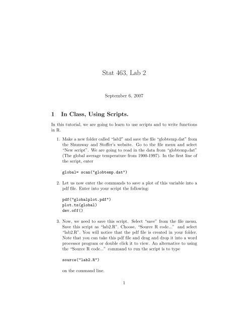
<strong>Stat</strong> <strong>463</strong>, <strong>Lab</strong> 2<br />
September 6, 2007<br />
1 In Class, Using Scripts.<br />
In this tutorial, we are going to learn to use scripts and to write functions<br />
in R.<br />
1. Make a new folder called “lab2” and save the file “globtemp.dat” from<br />
the Shumway and Stoffer’s website. Go to the file menu and select<br />
“New script”. We are going to read in the data from “globtemp.dat”<br />
(The global average temperature from 1900-1997). In the first line of<br />
the script, enter<br />
global= scan("globtemp.dat")<br />
2. Let us now enter the commands to save a plot of this variable into a<br />
pdf file. Enter into your script the following:<br />
pdf("globalplot.pdf")<br />
plot.ts(global)<br />
dev.off()<br />
3. Now, we need to save this script. Select “save” from the file menu.<br />
Save this script as “lab2.R”. Choose, “Source R code...” and select<br />
“lab2.R”. You will notice that the pdf file is created in your folder.<br />
Note that you can take this pdf file and drag and drop it into a word<br />
processor program or double click it to view. An alternative to using<br />
the “Source R code...” command to run the script is to type<br />
source("lab2.R")<br />
on the command line.<br />
1
4. We can add to the script by saving plots of this data differenced and<br />
also ACF plots of the data and the differenced data.<br />
globaldiff=diff(global)<br />
pdf("globaldiffplot.pdf")<br />
plot.ts(globaldiff)<br />
dev.off()<br />
pdf("globalacf.pdf")<br />
acf(global)<br />
dev.off()<br />
pdf("globaldiffacf.pdf")<br />
acf(globaldiff)<br />
dev.off()<br />
Save and run the script.<br />
2 In Class, Writing Functions.<br />
In this lab, we will learn to write our own functions in R. (If you would like<br />
more information about writing functions, see section 10 of An Introduction<br />
to R.) One important reason for learning about functions is to allow us to<br />
run simulations. In this section, we will write a function to simulate AR<br />
processes. For homework, you will write your own function to simulate MA<br />
processes.<br />
1. We will start by writing a very simple function, so we can learn how<br />
things work in R. Functions take arguments, do something to the arguments,<br />
and return a result. Start a new script titled “add.R”. Here<br />
is a short function to enter at the top of your script that will simply<br />
add two numbers and return the result.<br />
add=function(a,b){<br />
result=a+b<br />
result}<br />
Now, run your script. Then, type add(2,3), and notice the result.<br />
This function has two arguments, a and b. The result is returned by<br />
simply typing the object that you would like to have returned, in this<br />
case, the numerical variable result.<br />
2
2. Another example would be to write a function to simulate a Gaussian<br />
random walk. We will need to take arguments for the length of the<br />
series and the variance of the white noise process and return a vector<br />
representing the random walk. Here is one possible implementation:<br />
randomwalk=function(sigsq,T ){<br />
x=rep(0,T)<br />
w=rnorm(T,sd=sqrt(sigsq))<br />
for ( i in 2:T){<br />
x[i]=x[i-1]+w[i]<br />
}<br />
x<br />
}<br />
(Note that I am assuming an initial condition of zero.) Try a few<br />
sample paths, and calculate the ACF of those sample paths.<br />
3. Now, we will write a function to simulate an AR(p) process of length<br />
T . What information is necessary to do this? We will need the AR<br />
parameters φ 1 , ..., φ p , the variance of the white noise σ 2 , and the length<br />
of the time series we would like to generate T . These will be the<br />
arguments for our function.<br />
It would be nice if we could write one function that will generate an<br />
AR time series regardless of p. We will accomplish this by entering<br />
the AR parameters as a vector. Our function will be as follows:<br />
arsim=function(phis, sigsq, T){<br />
p=length(phis) #find the number of lags in our AR<br />
noise=rnorm(T+p, sd=sqrt(sigsq)) #generate the white noise plus a few to get started<br />
x=c(noise[1:p],rep(0,T)) #put the initial noise terms in and set the rest to zero<br />
for (i in (p+1):(T+p)){ #this loop generates the AR series with the recursive formula<br />
x[i]=phis %*% x[i-(1:p)] +noise[i]<br />
}<br />
x=x[(p+1):(T+p)] #throw away those initial starting points<br />
x #return the time series<br />
}<br />
We should walk through this function definition to make sure we understand<br />
things. First, we see that there are three arguments. The<br />
first argument is phis which is a vector containing the AR parameters<br />
in order: φ 1 , ..., φ p . The second is sigsq, the variance of the white<br />
noise, and the last is how many observations we want, T.<br />
3
The first line of the function finds the length of the phis which is<br />
p. We could pass an additional argument p, but this way is simpler.<br />
The second line generates T + p independent normal random variables<br />
with variance sigsq. In terms of how we have been writing our models,<br />
this command generates the w t . We generate p extra white noise<br />
terms to use as our initial values for the first p values of our time series.<br />
We have to start our series in some way, and this is not a completely<br />
ridiculous method. Later, we will come up with more clever ways to<br />
deal with this problem.<br />
We are going to use the variable x to store our time series. So, the<br />
next command sets up the vector x with the first p white noise terms<br />
and the rest zeros. The next set of statements is a for loop. This<br />
loop generates the time series using our recursive definition of an AR<br />
series. Note the operator %*%. This take the inner product of two<br />
vectors. In other words, the first element of vector one times the first<br />
element of vector two plus the second element of vector one times the<br />
second element of vector two plus and so on. The command after the<br />
for loop simply gets rid of those first p white noise terms leaving us<br />
with the AR process only. The final x returns our time series.<br />
4. Now that we have a function to generate an AR series, let us put it to<br />
work. Generate an AR(1) time series of length 200 and with φ 1 = 0.5<br />
and σ 2 = 1 using the command<br />
x1=arsim(c(0.5), 1,200)<br />
Take a look at a plot of the data and the ACF of this time series. Is<br />
this what you would expect?<br />
Also, generate a similar time series but with φ 1 = −0.5. How do the<br />
two time series look different? How about the ACF’s?<br />
5. We see with a |φ 1 | < 1 the process appears reasonable and stationary,<br />
and the last simulations you did confirmed that. Try a φ 1 of 1.1, 1.01,<br />
1.001, and 0.99. What do you notice?<br />
4
3 Homework<br />
1. Write a function called masim to generate a MA(q) series of length T .<br />
2. Make sure that your function works. Simulate a model with σ 2 = 1,<br />
θ 1 = 0.5, and θ 2 = 2 with T = 10, 000. Make an ACF plot. Is this<br />
consistent with the model that you generated? Try generating a model<br />
with the same parameters but only 200 observations. Make an ACF.<br />
Repeat this a few times, what do you notice about the autocorrelations<br />
and the dotted blue lines?<br />
3. Use the arsim() function from class to find one AR(2) that seems to<br />
be stationary and another that seems not to be stationary. Do this<br />
with simulations and plots of the simulations. Report the parameters,<br />
φ 1 and φ 2 , from your stationary and non-stationary models.<br />
5