JEST-M, Vol. 2, Issue 1, 2013 - MVJ College of Engineering

37 JEST-M, Vol. 2, Issue 1, 2013
pseudorandom bit which is 1 with probability 1/2. This
mechanism can mimic a probabilistic cellular automaton.
VIII. CASE-STUDY- THERMO-MECHANICALLY DEFORMED
COMPONENT MICROSTRUCTURE SIMULATION
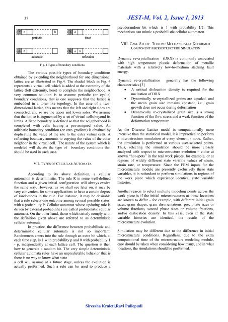
Fig. 4 Types of boundary conditions
The various possible types of boundary conditions
obtained by extending the neighborhood for one dimensional
lattice are as illustrated in Fig.4. The shaded block in Fig. 4
represents a virtual cell which is added at the extremity of the
lattice (left extremity, here) to complete the neighborhood. A
very common solution is to assume periodic (or cyclic)
boundary conditions, that is one supposes that the lattice is
embedded in a torus-like topology. In the case of a twodimensional
lattice, this means that the left and right sides are
connected, and so are the upper and lower sides. We assume
that the lattice is augmented by a set of virtual cells beyond its
limits. A fixed boundary is defined so that the neighborhood is
completed with cells having a pre-assigned value. An
adiabatic boundary condition (or zero-gradient) is obtained by
duplicating the value of the site to the extra virtual cells. A
reflecting boundary amounts to copying the value of the other
neighbor in the virtual cell. The nature of the system which is
modeled will dictate the type of boundary conditions that
should be used in each case.
VII. TYPES OF CELLULAR AUTOMATA
According to its above definition, a cellular
automaton is deterministic. The rule R is some well-defined
function and a given initial configuration will always evolve
the same way. However, as we shall see later on, it may be
very convenient for some applications to have a certain degree
of randomness in the rule. For instance, it may be desirable
that a rule selects one outcome among several possible states;
with a probability P. Cellular automata whose updating rule is
driven by external probabilities are called probabilistic cellular
automata. On the other hand, those which strictly comply with
the definition given above are referred to as deterministic
cellular automata.
In practice, the difference between probabilistic and
deterministic cellular automata is not so important.
Randomness enters into the rule through an extra bit which, at
each time step, is 1 with probability p and 0 with probability 1
- p, independently at each lattice cell. The question is then
how to generate a random bit. The very simple deterministic
cellular automata rules have an unpredictable behavior that is
there is no way to know what state
a cell will assume at a future stage, unless the evolution is
actually performed. Such a rule can be used to produce a
Dynamic re-crystallization (DRX) is commonly associated
with high temperature plastic deformation of metallic
materials with a relatively low-to-medium stacking fault
energy.
Dynamic re-crystallization generally has the following
characteristics [3]
A critical dislocation density is required for the
nucleation of DRX
Dynamically re-crystallized grains are equaled, and
the mean grain size remains constant, i.e., grain
growth does not occur during deformation
Dynamically re-crystallized grain size is a strong
function of the flow stress and a weak function of the
deformation temperature.
As the Discrete Lattice model is computationally more
intensive than the statistical model, it is impractical to perform
a microstructure simulation at every element / node. Rather,
the simulation is performed at various user-selected points.
Thus, selecting the simulation should be more closely
analyzed with respect to microstructure evolution – either at
known “hot-spots” in the real work pieces, for example, or at
regions of widely different state variable values of strain,
strain rate, or temperature. Since the FEM inputs for the
microstructure module are presently exclusively these state
variables, it is redundant to perform simulations in regions of
the work piece which experience identical state variable
histories.
Another reason to select multiple modeling points across the
work piece is if the initial microstructures at those locations
are known to differ – for example, with different initial grain
sizes, grain shapes, grain disorientations, precipitate sizes or
volume fractions, second phase sizes or volume fractions,
and/or dislocation density. In this case, even if the state
variable histories are identical, the results of the
microstructure evolution.
Simulation may be different due to the difference in initial
microstructure conditions. Regardless, due to the extra
computational time of the microstructure modeling module,
care should be taken when considering how many, and in what
locations, the simulations should be performed.
Sireesha Kraleti,Ravi Pullepudi