JEST-M, Vol. 2, Issue 1, 2013 - MVJ College of Engineering
JEST-M, Vol. 2, Issue 1, 2013 - MVJ College of Engineering
JEST-M, Vol. 2, Issue 1, 2013 - MVJ College of Engineering

Create successful ePaper yourself
Turn your PDF publications into a flip-book with our unique Google optimized e-Paper software.
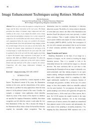
34 <strong>JEST</strong>-M, <strong>Vol</strong>. 2, <strong>Issue</strong> 1, <strong>2013</strong><br />
Micro-Structure Simulation using Cellular Automata:<br />
A Case Study<br />
Sireesha Kraleti 1<br />
Asst. Pr<strong>of</strong>essor, IEM Department, <strong>MVJ</strong> <strong>College</strong> <strong>of</strong><br />
<strong>Engineering</strong>, Bangalore-67, India<br />
siree.reesha@gmail.com<br />
Abstract—Dynamic re-crystallization governs the plastic flow<br />
behavior and the final microstructure <strong>of</strong> many crystalline<br />
materials during thermo-mechanical processing. Understanding<br />
the re-crystallization process is the key to linking dislocation<br />
activities at the microscopic scale to mechanical properties at the<br />
macroscopic scale. A modeling methodology coupling<br />
fundamental metallurgical principles with the cellular automaton<br />
(CA) technique is used to simulate the dynamic re-crystallization<br />
process. Cellular automata (CA) are a class <strong>of</strong> spatially and<br />
temporally discrete, deterministic mathematical systems<br />
characterized by local interaction and an inherently parallel<br />
form <strong>of</strong> evolution. Microstructure simulation predicts the<br />
nucleation and the growth kinetics <strong>of</strong> dynamically re-crystallized<br />
grains. Hence it can simulate different stages <strong>of</strong> micro-structural<br />
evolution during thermo-mechanical processing. This paper<br />
illustrates the simulated micro structure result <strong>of</strong> at selected<br />
regions on the thermo-mechanically deformed component.<br />
Index Terms—Cellular Automata, Microstructure Simulation,<br />
Dynamic Re-crystallization. (key words)<br />
I. INTRODUCTION<br />
Cellular automata (CA) are, fundamentally, the<br />
simplest mathematical representations <strong>of</strong> a much broader class<br />
<strong>of</strong> complex systems where, for the moment, "complex system”<br />
means any dynamical system that consists <strong>of</strong> more nonlinearly<br />
interacting parts. As such, CA have proven to be extremely<br />
useful idealizations <strong>of</strong> the dynamical behavior <strong>of</strong> many real<br />
complex systems, including physical fluids, neural networks,<br />
molecular dynamical systems, natural ecologies, military<br />
command and control networks, and the economy, among<br />
many others. Because <strong>of</strong> their underlying simplicity, CA are<br />
also powerful conceptual engines with which to study general<br />
pattern formation. They have already provided critical insights<br />
into the self-organization <strong>of</strong> chemical reaction-diffusion<br />
systems, crystal growth, pattern formation on seashells, and<br />
phase-transition-like phenomena in vehicular traffic flow, to<br />
name but a few examples. On a more practical side, CA may<br />
provide the basis for extremely powerful encryption<br />
algorithms, a subject about which there has recently been<br />
much heated debate. So, the cellular automata technique is<br />
used for the simulation <strong>of</strong> the micro-structure in the flow<br />
forming process.<br />
Cellular automata (<strong>of</strong>ten termed CA) are an<br />
idealization <strong>of</strong> a physical system in which space and time are<br />
Ravi Pullepudi 2<br />
Asst. Systems Engineer, TCS <strong>Engineering</strong> and Industrial<br />
Services, GR Tech. Park, Bangalore-67, India.<br />
ravipullepudi@gmail.com<br />
discrete, and the physical quantities take only a finite set <strong>of</strong><br />
values. Although cellular automata have been reinvented<br />
several times (<strong>of</strong>ten under different names), the concept <strong>of</strong> a<br />
cellular automaton dates back from the late 1940s. During the<br />
following fifty years <strong>of</strong> existence, cellular automata have<br />
been developed and used in many different fields.<br />
Cellular automata (CA) are a class <strong>of</strong> spatially and<br />
temporally discrete, deterministic mathematical systems<br />
characterized by local interaction and an inherently parallel<br />
form <strong>of</strong> evolution. First introduced by von Neumann in the<br />
early 1950s to act as simple models <strong>of</strong> biological selfreproduction,<br />
CA are prototypical models for complex<br />
systems and processes consisting <strong>of</strong> a large number <strong>of</strong><br />
identical, simple, locally interacting components. The study <strong>of</strong><br />
these systems has generated great interest over the years<br />
because <strong>of</strong> their ability to generate a rich spectrum <strong>of</strong> very<br />
complex patterns <strong>of</strong> behavior out <strong>of</strong> sets <strong>of</strong> relatively simple<br />
underlying rules. Moreover, they appear to capture many<br />
essential features <strong>of</strong> complex self-organizing cooperative<br />
behavior observed in real systems.<br />
II. TERMINOLOGY<br />
Discrete lattice <strong>of</strong> cells: the system substrate consists<br />
<strong>of</strong> a one-, two- or three dimensional lattices <strong>of</strong> cells.<br />
Homogeneity: all cells are equivalent.<br />
Discrete states: each cell takes on one <strong>of</strong> a finite<br />
number <strong>of</strong> possible discrete states.<br />
Local interactions: each cell interacts only with cells<br />
that are in its local neighbourhood, discrete<br />
dynamics: at each discrete unit time, each cell<br />
updates its current state according to a transition rule<br />
taking into account the states <strong>of</strong> cells in its<br />
neighbourhood.<br />
III. WHY TO STUDY CA? [1]<br />
There are at least four partially overlapping<br />
motivations for studying CA, which we order according to<br />
increasing levels <strong>of</strong> theoretical significance<br />
As powerful computation engines<br />
As discrete dynamical system simulators<br />
Sireesha Kraleti,Ravi Pullepudi
35 <strong>JEST</strong>-M, <strong>Vol</strong>. 2, <strong>Issue</strong> 1, <strong>2013</strong><br />
As conceptual vehicles for studying pattern formation<br />
and complexity<br />
As original models <strong>of</strong> fundamental physics<br />
A. CA as Powerful Computation Engines<br />
СA allow very efficient parallel computational<br />
implementations to be made <strong>of</strong> lattice models in physics and<br />
thus for a detailed analysis <strong>of</strong> many concurrent dynamical<br />
processes in nature. Indeed, dedicated hardware represents one<br />
<strong>of</strong> the most promising practical applications <strong>of</strong> CA modeling.<br />
With the help <strong>of</strong> such hardware, many heret<strong>of</strong>ore intractable<br />
but technologically important problems such as fluid flow near<br />
and around airplane wings, are becoming computationally<br />
accessible for the first time.<br />
B. CA as Discrete Dynamical System Simulators<br />
CA allows systematic investigation <strong>of</strong> complex<br />
phenomena by embodying any number <strong>of</strong> desirable physical<br />
properties. Reversible CA, for example, can be used as<br />
laboratories for studying the relationship between microscopic<br />
rules and macroscopic behavior- exact computability ensuring<br />
that the memory <strong>of</strong> the initial state is retained exactly for<br />
arbitrarily long periods <strong>of</strong> time. Discrete models <strong>of</strong> turbulence<br />
are particularly impressive in that they clearly show that very<br />
simple finite dynamical implementations <strong>of</strong> local conservation<br />
laws (defined so that the discrete system is computationally<br />
universal) are capable <strong>of</strong> exactly reproducing continuum<br />
system behavior on the micro scale.<br />
C. CA as Conceptual Vehicles for Exploring Pattern<br />
Formation<br />
CA can be treated as abstract discrete dynamical<br />
systems embodying intrinsically interesting, and potentially<br />
novel, behavioral features. The central motivation is to<br />
abstract the general principles governing self-organizing<br />
structure formation. Related interests include formal<br />
classification <strong>of</strong> the dynamical behavior <strong>of</strong> complex systems; a<br />
better understanding <strong>of</strong> the relationship between the dynamics<br />
<strong>of</strong> continuous and discrete systems; and the quantification <strong>of</strong><br />
complexity-as a system property. All <strong>of</strong> these questions are<br />
particularly accessible through studying the generic behavior<br />
<strong>of</strong> СA systems.<br />
D. CA as Original Models <strong>of</strong> Fundamental Physics<br />
CA allows studies <strong>of</strong> radically new discrete<br />
dynamical approaches to microscopic physics, exploring the<br />
possibility that nature locally and digitally processes its own<br />
future states. This paper is devoted to a prolonged discussion<br />
<strong>of</strong> such potentially ground breaking models <strong>of</strong> physics. Using<br />
the fact that computationally universal systems are capable <strong>of</strong><br />
arbitrarily complicated behavior (in the sense that they can<br />
mimic any computation performed by a conventional<br />
computer), the idea is to construct fundamentally discrete field<br />
theories to compete with existing continuous models. The<br />
emphasis in this class <strong>of</strong> models is emphatically not to<br />
construct a lattice-gauge-like theory; rather, in the same way<br />
as lattice gas CA successfully reproduce continuous fluid flow<br />
despite never having heard <strong>of</strong> the Navier-Stokes equations, so<br />
the hope is to abstract a set <strong>of</strong> microphysical laws that<br />
reproduce known behavior on the macro scale.<br />
IV. REQUIREMENTS OF CELLULAR AUTOMATA [2]<br />
A Cellular Automation generally requires<br />
A regular lattice <strong>of</strong> cells covering a portion <strong>of</strong> a d-<br />
dimensional space.<br />
A set ф (r', t) = { ф 1(r', t), ф 2(r', t), ф 3(r', t)................<br />
ф m(r', t)} <strong>of</strong> Boolean variables attached to each site r<br />
<strong>of</strong> the lattice and giving the local state r’ <strong>of</strong> each cell<br />
at the time t = 0, 1, 2,....<br />
A rule R = {R 1 , R 2 ..... R m } which specifies the time<br />
evolution <strong>of</strong> the state's ф (r',t) in the following way as<br />
shown in Eq. (4.1).<br />
(r ', t 1) R ( (r ', t), (r ' 1, t), (r ' 2, t),.... (r ' q, t))<br />
j<br />
j<br />
Where in Eq. (1) r' k designate the cells<br />
belonging to a given neighborhood <strong>of</strong> cell r'. In the above<br />
definition, the rule R is identical for all sites and is applied<br />
simultaneously to each <strong>of</strong> them, leading to a synchronous<br />
dynamics. It is important to notice that the rule is<br />
homogeneous, that is it cannot depend explicitly on the cell<br />
position r. However, spatial (or even temporal) in<br />
homogeneities can be introduced by having some<br />
(r ') systematically 1 in some given locations <strong>of</strong> the lattice<br />
j<br />
to mark particular cells for which a different rule applies.<br />
Boundary cells are a typical example <strong>of</strong> spatial in<br />
homogeneity. Similarly, it is easy to alternate between two<br />
rules by having a bit which is 1 at even time steps and 0 at odd<br />
time steps. In our definition, the new state at time t + 1 is only<br />
a function <strong>of</strong> the previous state at time t. It is sometimes<br />
necessary to have a longer memory and introduce a<br />
dependence on the states at time t - l, t - 2,..., t -k. Such a<br />
situation is already included in the definition if one keeps a<br />
copy <strong>of</strong> the previous states in the current state.<br />
V. NEIGHBOURHOODS (NH)<br />
A cellular automata rule is local, by definition. The<br />
updating <strong>of</strong> a given cell requires one to know only the state <strong>of</strong><br />
the cells in its vicinity. The spatial region in which a cell<br />
needs to search is called the neighborhood. In principle, there<br />
(1)<br />
Sireesha Kraleti,Ravi Pullepudi
36 <strong>JEST</strong>-M, <strong>Vol</strong>. 2, <strong>Issue</strong> 1, <strong>2013</strong><br />
is no restriction on the size <strong>of</strong> the neighborhood, except that it<br />
is the same for all cells. However, in practice, it is <strong>of</strong>ten made<br />
up <strong>of</strong> adjacent cells only. If the neighborhood is too large, the<br />
complexity <strong>of</strong> the rule may be unacceptable as the complexity<br />
usually grows exponentially fast with the number <strong>of</strong> cells in<br />
the neighborhood (NH).<br />
For two-dimensional cellular automata, two<br />
neighborhoods are <strong>of</strong>ten considered, the von Neumann<br />
neighborhood, which consists <strong>of</strong> a central cell (the one which<br />
is to be updated) and its four geographical neighbors north,<br />
west, south and east as shown in Fig. 1. The Moore<br />
neighborhood contains, in addition, second nearest neighbors<br />
north-east, north-west, south-east and south-west, that is a<br />
total <strong>of</strong> nine cells as shown in Fig. 2<br />
Fig. 1 Von Neumann NH<br />
Where in Figs.1 and 2, the shaded region indicates<br />
the central cell which is updated according to the state <strong>of</strong> the<br />
cells located within the domain marked with the bold line.<br />
Another useful neighborhood is the so-called<br />
Margolus neighborhood which allows a partitioning <strong>of</strong> space<br />
and a reduction <strong>of</strong> rule complexity. The space is divided into<br />
adjacent blocks <strong>of</strong> two-by-two cells. The rule is sensitive to<br />
the location within this so-called Margolus block, namely<br />
upper-left, upper-right, lower-left and lower-right. The way<br />
the lattice is partitioned changes as the rule is iterated. It<br />
alternates between an odd and an even partition, as shown in<br />
Fig. 3. As a result, information can propagate outside the<br />
boundaries <strong>of</strong> the blocks, as evolution takes place. The key<br />
idea <strong>of</strong> the Margolus neighborhood is that when updating<br />
occurs, the cells within a block evolve only according to the<br />
state <strong>of</strong> that block and do not immediately depend on what is<br />
in the adjacent blocks. To understand this property, consider<br />
the difference with the situation <strong>of</strong> the Moore neighborhood<br />
shown in Fig. 4.3 After iteration, the cell located on the west<br />
<strong>of</strong> the shaded cell will evolve relatively to its own Moore<br />
neighborhood. Therefore, the cells within a given Moore<br />
neighborhood evolve according to the cells located in a wider<br />
region. The purpose <strong>of</strong> space partitioning is to prevent these<br />
"long distance" effects from occurring.<br />
In Fig.3, the lattice is partitioned in 2 x 2 blocks. Two<br />
partitioning are possible - odd and even partitions, as shown<br />
by the blocks delimited by the solid and broken lines,<br />
respectively. The neighborhood alternates between these two<br />
situations, at even and odd time steps. Within a block, the cells<br />
are distinguishable and are labeled ul, ur, 11 and lr for upperleft,<br />
upper-right, lower-left and lower-right. The cell labeled lr<br />
in the figure will be become ul, at the next iteration, with the<br />
alternative partitioning.<br />
VI. BOUNDARY CONDITIONS<br />
Fig. 2 Moore NH<br />
In practice, when simulating a given cellular<br />
automata rule, one cannot deal with an infinite lattice. The<br />
system must be finite and have boundaries. Clearly, a site<br />
belonging to the lattice boundary does not have the same<br />
neighborhood as other internal sites. In order to define the<br />
behavior <strong>of</strong> these sites, a different evolution rule can be<br />
considered, which sees the appropriate neighborhood. This<br />
means that the information <strong>of</strong> being, or not, at a boundary is<br />
coded at the site and, depending on this information, a<br />
different rule is selected. Following this approach, it is also<br />
possible to define several types <strong>of</strong> boundaries, all with<br />
different behavior. Instead <strong>of</strong> having a different rule at the<br />
limits <strong>of</strong> the system, another possibility is to extend the<br />
neighborhood for the sites at the boundary.<br />
Fig. 3 Margolus NH<br />
Sireesha Kraleti,Ravi Pullepudi
37 <strong>JEST</strong>-M, <strong>Vol</strong>. 2, <strong>Issue</strong> 1, <strong>2013</strong><br />
pseudorandom bit which is 1 with probability 1/2. This<br />
mechanism can mimic a probabilistic cellular automaton.<br />
VIII. CASE-STUDY- THERMO-MECHANICALLY DEFORMED<br />
COMPONENT MICROSTRUCTURE SIMULATION<br />
Fig. 4 Types <strong>of</strong> boundary conditions<br />
The various possible types <strong>of</strong> boundary conditions<br />
obtained by extending the neighborhood for one dimensional<br />
lattice are as illustrated in Fig.4. The shaded block in Fig. 4<br />
represents a virtual cell which is added at the extremity <strong>of</strong> the<br />
lattice (left extremity, here) to complete the neighborhood. A<br />
very common solution is to assume periodic (or cyclic)<br />
boundary conditions, that is one supposes that the lattice is<br />
embedded in a torus-like topology. In the case <strong>of</strong> a twodimensional<br />
lattice, this means that the left and right sides are<br />
connected, and so are the upper and lower sides. We assume<br />
that the lattice is augmented by a set <strong>of</strong> virtual cells beyond its<br />
limits. A fixed boundary is defined so that the neighborhood is<br />
completed with cells having a pre-assigned value. An<br />
adiabatic boundary condition (or zero-gradient) is obtained by<br />
duplicating the value <strong>of</strong> the site to the extra virtual cells. A<br />
reflecting boundary amounts to copying the value <strong>of</strong> the other<br />
neighbor in the virtual cell. The nature <strong>of</strong> the system which is<br />
modeled will dictate the type <strong>of</strong> boundary conditions that<br />
should be used in each case.<br />
VII. TYPES OF CELLULAR AUTOMATA<br />
According to its above definition, a cellular<br />
automaton is deterministic. The rule R is some well-defined<br />
function and a given initial configuration will always evolve<br />
the same way. However, as we shall see later on, it may be<br />
very convenient for some applications to have a certain degree<br />
<strong>of</strong> randomness in the rule. For instance, it may be desirable<br />
that a rule selects one outcome among several possible states;<br />
with a probability P. Cellular automata whose updating rule is<br />
driven by external probabilities are called probabilistic cellular<br />
automata. On the other hand, those which strictly comply with<br />
the definition given above are referred to as deterministic<br />
cellular automata.<br />
In practice, the difference between probabilistic and<br />
deterministic cellular automata is not so important.<br />
Randomness enters into the rule through an extra bit which, at<br />
each time step, is 1 with probability p and 0 with probability 1<br />
- p, independently at each lattice cell. The question is then<br />
how to generate a random bit. The very simple deterministic<br />
cellular automata rules have an unpredictable behavior that is<br />
there is no way to know what state<br />
a cell will assume at a future stage, unless the evolution is<br />
actually performed. Such a rule can be used to produce a<br />
Dynamic re-crystallization (DRX) is commonly associated<br />
with high temperature plastic deformation <strong>of</strong> metallic<br />
materials with a relatively low-to-medium stacking fault<br />
energy.<br />
Dynamic re-crystallization generally has the following<br />
characteristics [3]<br />
A critical dislocation density is required for the<br />
nucleation <strong>of</strong> DRX<br />
Dynamically re-crystallized grains are equaled, and<br />
the mean grain size remains constant, i.e., grain<br />
growth does not occur during deformation<br />
Dynamically re-crystallized grain size is a strong<br />
function <strong>of</strong> the flow stress and a weak function <strong>of</strong> the<br />
deformation temperature.<br />
As the Discrete Lattice model is computationally more<br />
intensive than the statistical model, it is impractical to perform<br />
a microstructure simulation at every element / node. Rather,<br />
the simulation is performed at various user-selected points.<br />
Thus, selecting the simulation should be more closely<br />
analyzed with respect to microstructure evolution – either at<br />
known “hot-spots” in the real work pieces, for example, or at<br />
regions <strong>of</strong> widely different state variable values <strong>of</strong> strain,<br />
strain rate, or temperature. Since the FEM inputs for the<br />
microstructure module are presently exclusively these state<br />
variables, it is redundant to perform simulations in regions <strong>of</strong><br />
the work piece which experience identical state variable<br />
histories.<br />
Another reason to select multiple modeling points across the<br />
work piece is if the initial microstructures at those locations<br />
are known to differ – for example, with different initial grain<br />
sizes, grain shapes, grain disorientations, precipitate sizes or<br />
volume fractions, second phase sizes or volume fractions,<br />
and/or dislocation density. In this case, even if the state<br />
variable histories are identical, the results <strong>of</strong> the<br />
microstructure evolution.<br />
Simulation may be different due to the difference in initial<br />
microstructure conditions. Regardless, due to the extra<br />
computational time <strong>of</strong> the microstructure modeling module,<br />
care should be taken when considering how many, and in what<br />
locations, the simulations should be performed.<br />
Sireesha Kraleti,Ravi Pullepudi
38 <strong>JEST</strong>-M, <strong>Vol</strong>. 2, <strong>Issue</strong> 1, <strong>2013</strong><br />
Fig. 1. Fig5. (a). Grain orientation<br />
(b).Dislocation density<br />
(c). Grain boundaries<br />
(d). Grain orientation + Grain boundaries<br />
Fig.5 shows the simulated micro structure result <strong>of</strong> the<br />
selected point 1 on the thermo-mechanically deformed<br />
component.<br />
IX. CONCLUSION:<br />
A CA technique coupled with metallurgical principles has<br />
enabled accurate simulation <strong>of</strong> micro structural evolution<br />
during DRX <strong>of</strong> metallic materials. This technique is used for<br />
simulating the microstructure <strong>of</strong> the thermo mechanically<br />
processed components. Microstructure simulation predicts the<br />
nucleation and the growth kinetics <strong>of</strong> dynamically<br />
recrystallised grains, orientation and dislocation density.<br />
REFERENCES<br />
[1]. Andrew Ilachinski, A text book on " Cellular Automata-A<br />
Discrete Universe ". World Scientific Publishing Co. Pte.<br />
Ltd.,2001.<br />
[2]. Bastien Chopard and Michel Droz, A text book on<br />
"Cellular Automata - Modeling <strong>of</strong> Physical Systems".<br />
Cambridge University press, 1998.<br />
[3]. R. Ding, Z.X. Guo “Modelling <strong>of</strong> dynamic recrystallization<br />
using an extended cellular automaton<br />
approach”. Computational Materials Science 23 (2002) 209–<br />
218.<br />
[4]. Ravi Pullepudi, A. Gopala Krishna “Finite Element<br />
Simulation <strong>of</strong> a Flow Forming Process for an Aerospace<br />
Component”, M.Tech Thesis, JNTU K, Kakinada, 2011.<br />
[5]. Google and Wikipedia.<br />
Sireesha Kraleti,Ravi Pullepudi