1 Introduction 2 Resolvents and Green's Functions

(c) Notice that, using
G(x, y; z) =
∞∑
k=1
φ k (x)φ ∗ k(y)
, (123)
ω k − z
the normalized eigenstate, φ k (x), can be obtained by evaluating
the residue of G at the pole z = ω k . Do this calculation, and check
that your result is properly normalized.
(d) Consider the limit a → −∞, b → ∞. Show, in this limit that
G(x, y; z) tends to the Green’s function we obtain in this note for
this Hamiltonian on x ∈ (−∞, ∞):
G(x, y; z) = i√ m
2z eiρ|x−y| . (124)
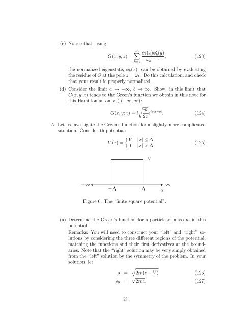
5. Let us investigate the Green’s function for a slightly more complicated
situation. Consider th potential:
{ V |x| ≤ ∆
V (x) =
(125)
0 |x| > ∆
V
_ ∞
_ Δ
Δ
x
∞
Figure 6: The “finite square potential”.
(a) Determine the Green’s function for a particle of mass m in this
potential.
Remarks: You will need to construct your “left” and “right” solutions
by considering the three different regions of the potential,
matching the functions and their first derivatives at the boundaries.
Note that the “right” solution may be very simply obtained
from the “left” solution by the symmetry of the problem. In your
solution, let
√
ρ = 2m(z − V ) (126)
ρ 0 = √ 2mz. (127)
21