Spectral decomposition of seismic data with ... - Sigmacubed.com

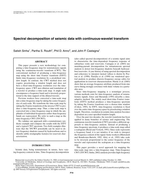
GEOPHYSICS, VOL. 70, NO. 6 (NOVEMBER-DECEMBER 2005); P. P19–P25,9FIGS.
10.1190/1.2127113
Spectral decomposition of seismic data with continuous-wavelet transform
Satish Sinha 1 , Partha S. Routh 2 , Phil D. Anno 3 , and John P. Castagna 1
ABSTRACT
This paper presents a new methodology for computing
a time-frequency map for nonstationary signals
using the continuous-wavelet transform (CWT). The
conventional method of producing a time-frequency
map using the short time Fourier transform (STFT)
limits time-frequency resolution by a predefined window
length. In contrast, the CWT method does not
require preselecting a window length and does not
have a fixed time-frequency resolution over the timefrequency
space. CWT uses dilation and translation of
a wavelet to produce a time-scale map. A single scale
encompasses a frequency band and is inversely proportional
to the time support of the dilated wavelet.
Previous workers have converted a time-scale map
into a time-frequency map by taking the center frequencies
of each scale. We transform the time-scale map by
taking the Fourier transform of the inverse CWT to produce
a time-frequency map. Thus, a time-scale map is
converted into a time-frequency map in which the amplitudes
of individual frequencies rather than frequency
bands are represented. We refer to such a map as the
time-frequency CWT (TFCWT).
We validate our approach with a nonstationary synthetic
example and compare the results with the STFT
and a typical CWT spectrum. Two field examples illustrate
that the TFCWT potentially can be used to detect
frequency shadows caused by hydrocarbons and to
identify subtle stratigraphic features for reservoir characterization.
INTRODUCTION
Seismic data, being nonstationary in nature, have varying
frequency content in time. Time-frequency decomposition
(also called spectral decomposition) of a seismic signal aims
to characterize the time-dependent frequency response of
subsurface rocks and reservoirs. Castagna et al. (2003) use
matching-pursuit decomposition for instantaneous spectral
analysis to detect low-frequency shadows beneath hydrocarbon
reservoirs. A case history of using spectral decomposition
and coherency to interpret incised valleys is shown by Peyton
et al. (1998). Partyka et al. (1999) use windowed spectral
analysis to produce discrete-frequency energy cubes for
applications in reservoir characterization. Hardy et al. (2003)
show that an average frequency attribute produced from sine
curve-fitting strongly correlates with shale volume in a particular
area.
Since time-frequency mapping is a nonunique process,
various methods exist for time-frequency analysis of nonstationary
signals. Jones and Baraniuk (1995) describe a dataadaptive
method. The widely used short-time Fourier transform
(STFT) method produces a time-frequency spectrum
by taking the Fourier transform over a chosen time window
(Cohen, 1995). In STFT, time-frequency resolution is fixed
over the entire time-frequency space by preselecting a window
length. Therefore, resolution in seismic data analysis becomes
dependent on a user-specified window length.
Over the past two decades, the wavelet transform has been
applied in many branches of science and engineering. The
continuous-wavelet transform (CWT) provides a different approach
to time-frequency analysis. Instead of producing a
time-frequency spectrum, it produces a time-scale map called
a scalogram (Rioul and Vetterli, 1991). Since scale represents
a frequency band, it is not intuitive if we wish to interpret
the frequency content of the signal. Some workers (Hlawatsch
and Boudreaux-Bartels, 1992; Abry et al., 1993) take scale
to be inversely proportional to the center frequency of the
wavelet and represented the scalogram as a time-frequency
map.
This paper provides a novel approach for mapping the
time-scale map into a time-frequency map. Time-frequency
CWT (TFCWT; Sinha, 2002) analysis provides high-frequency
Manuscript received by the Editor October 21, 2003; revised manuscript received March 15, 2005; published online October 12, 2005.
1
University of Oklahoma, School of Geology and Geophysics, 100 E. Boyd St., 810 SEC, Norman, Oklahoma 73019. E-mail: satish@ou.edu;
jcastagnaou@yahoo.com.
2
Boise State University, Department of Geosciences, Boise, Idaho 83725. E-mail: prouth@boisestate.edu.
3
ConocoPhillips, Seismic Imaging and Prediction, 600 N. Dairy Ashford, Houston, Texas 77252-2197. E-mail: phil.d.anno@conocophillips.com.
c○ 2005 Society of Exploration Geophysicists. All rights reserved.
P19

P20
Sinha et al.
resolution at low frequencies and high time resolution at high
frequencies. This optimal time-frequency resolution property
of the TFCWT makes it useful in seismic data analysis.
Computing the TFCWT in the Fourier domain is a fast process.
Furthermore, TFCWT is an invertible process such that
the inverse Fourier transform of the time summation of the
TFCWT reconstructs the original signal, provided the inverse
wavelet transform exists. For our purposes we require only the
forward transform; reproducibility is not a strict requirement.
Seismic data analysts sometimes observe low-frequency
shadows in association with hydrocarbon reservoirs. The
shadow is probably caused by attenuation of high-frequency
energy in the reservoir itself (Dilay and Eastwood, 1995;
Mitchell et al., 1997), such that the local dominant frequency
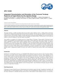
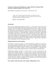
Figure 1. A chirp signal consisting of two known hyperbolic sweep frequencies with
constant amplitude for each frequency.
moves toward the low-frequency range. Thus, anomalous lowfrequency
energy is concentrated at or beneath the reservoir
level. The low frequencies are probably not caused by
inelastic attenuation. Ebrom (2004) lists about ten possible
mechanisms. High-frequency resolution at low frequencies,
given by the TFCWT, helps detect these shadows. On the
other hand, high time resolution at high frequencies can enhance
stratigraphic features from seismic data. Marfurt and
Kirlin (2001) investigate how tuning frequency varies with
thickness and use spectrally decomposed data to resolve thin
beds.
In this paper, we derive a formula to convert a scalogram
to a TFCWT. We begin by comparing the TFCWT spectrum
for a hyperbolic chirp signal with the CWT spectrum and the
STFT. Then we calculate TFCWT spectra
for two real data sets, one from Nigeria
and another publicly available from the
Stratton field, south Texas. In the first example,
we show that single-frequency visualization
of a seismic section in the frequency
domain with the TFCWT reveals
low-frequency anomalies associated with
hydrocarbon reservoirs. In the second example,
we show that single-frequency slices
along a horizon can be used to enhance
stratigraphic features.
TIME-FREQUENCY MAP FROM STFT
The Fourier transform f ˆ(ω) of a signal f (t) is the inner
product of the signal with the basis function e iωt , i.e.,
∫ ∞
f ˆ(ω) =〈f (t),e iωt 〉= f (t)e −iωt dt, (1)
−∞
where t is time. A seismic signal, when transformed into the
frequency domain using the Fourier transform, gives the overall
frequency behavior; such a transformation is inadequate
for analyzing a nonstationary signal. We can include the time
dependence by windowing the signal (i.e., taking short segments
of the signal) and then performing the Fourier transform
on the windowed data to obtain local frequency information.
Such an approach of time-frequency analysis is called the
short-time Fourier transform (STFT), and the time-frequency
map is called a spectrogram (Cohen, 1995). The STFT is given
by the inner product of the signal f (t) with a time-shifted window
function φ(t). Mathematically, it can be expressed as
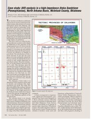
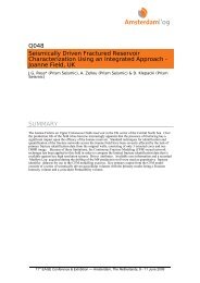
Figure 2. A spectrogram of the chirp signal using a 400-ms
window length. Notice that the lower frequencies are well resolved
but the higher frequencies are not resolved.
ST FT (ω,τ) =〈f (t),φ(t − τ)e iωt 〉
=
∫ ∞
f (t) ¯φ(t − τ)e −iωt dt, (2)
−∞
where the window function φ is centered at time t = τ, with τ
being the translation parameter, and ¯φ is the complex conjugate
of φ.
We show a spectrogram computed for a chirp signal (Figure
1) with two hyperbolic frequency sweeps in Figure 2. We
use a 400-ms-long Hanning window for this computation. Note
in the spectrogram that the low frequencies are well resolved
and the high frequencies are either poorly resolved or not visible
at all. The reason is because the frequency resolution is

Time-Frequency Decomposition
P21
fixed by the preselected window length and is recognized as
the fundamental problem of the STFT in spectral analysis of a
nonstationary signal.
TIME-FREQUENCY MAP FROM CWT (TFCWT)
The CWT is an alternative method to analyze a signal. In
the CWT, wavelets dilate in such a way that the time support
changes for different frequencies. Smaller time support
increases the frequency support, which shifts toward higher
frequencies. Similarly, larger time support decreases the frequency
support, which shifts toward lower frequencies. Thus,
when the time resolution increases, the frequency resolution
decreases, and vice versa (Mallat, 1999).
A wavelet is defined as a function ψ(t) ∈ L 2 (R) withazero
mean, localized in both time and frequency. By dilating and
translating this wavelet ψ(t), we produce a family of wavelets:
ψ σ,τ (t) = 1 √ σ
ψ
( t − τ
σ
)
, (3)
where σ, τ ∈Rand σ is not zero and σ is the dilation parameter
or scale. Note that the wavelet is normalized such that the L2-
norm ‖ψ‖ is equal to unity. The CWT is defined as the inner
product of the family of wavelets ψ σ,τ (t)with the signalf (t).
This is given by
∫ ∞
F W (σ, τ) =〈f (t),ψ σ,τ (t)〉= f (t) 1 ( t − τ
√ ¯ψ
−∞ σ σ
(4)
where ¯ψ is the complex conjugate of ψ and F W (σ, τ) isthe
time-scale map (i.e., the scalogram). The convolution integral
in equation 4 can be computed easily in the Fourier domain.
The choice for the scale and the translation parameter can be
arbitrary, and we can choose to represent it any way we like.
To reconstruct the function f (t) from the wavelet transform,
we use Calderon’s identity (Daubechies, 1992), given by
f (t) = 1 ∫ ∞ ∫ ∞
( ) t − τ dσ dτ
F W (σ, τ)ψ
√ .
C ψ −∞ −∞
σ σ 2 (5) σ
For the inverse transform to exist, we require that the analyzing
wavelet satisfy the admissibility condition, given by
∫ ∞
| ˆψ(ω)| 2
C ψ = 2π
dω < ∞, (6)
−∞ ω
)
dt,
time-scale map, in terms of a time-frequency map, a number
of approaches can be taken. The easiest step would be
to stretch the scale to an equivalent frequency, depending
on the scale-frequency mapping of the wavelet. Typically for
time-frequency analysis, one converts a scalogram to a timefrequency
spectrum using f c /f ,where,f c is the center frequency
of the wavelet (Hlawatsch and Bartels, 1992). Such
a typical CWT spectrum of the chirp signal using the Morlet
wavelet is shown in Figure 3. However, we take an alternative
approach and compute a frequency spectrum of the signal
using the wavelet as an adaptive window. Because of the Morlet
wavelet’s dilation property, it is a natural window for signals
that require high-frequency resolution at low frequencies
and high time resolution at high frequencies. The translation
property allows us to examine the frequency content at various
times, thus leading to a time-frequency map that is adaptive
to the nonstationary nature of seismic signals. This timefrequency
map is obtained by taking the Fourier transform of
the inverse continuous wavelet transform.
Replacing f (t) from equation 5 into equation 1 gives
∫ ∞ ∫ ∞
1
−∞ −∞ σ 2√ σ
( t − τ
× F W (σ, τ)ψ
σ
f ˆ(ω) = 1 ∫ ∞
C ψ −∞
)
e −iωt dσ dτ dt. (8)
where ˆψ(ω) is the Fourier transform of ψ(t) andwhereC ψ
is a constant for wavelet ψ. The integrand in equation 6
has an integrable discontinuity at ω = 0 and also implies
that ∫ ψ(t)dt = 0. A commonly used wavelet in continuouswavelet
transform is the Morlet wavelet, defined as (Torrence
and Compo, 1998)
ψ 0 (t) = π −1/4 e iω 0t e −t2 /2 , (7)
where ω 0 is the frequency and is taken as 2π to satisfy the
admissibility condition. The center frequency of the Morlet
wavelet being inversely proportional to the scale provides an
easy interpretation from scale to frequency.
We note that a scale represents a frequency band and not
a single frequency. The scalogram does not provide a direct
intuitive interpretation of frequency. To interpret the
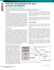
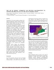
Figure 3. A typical CWT spectrum obtained for the chirp signal
shown in Figure 1. It is converted from the scalogram, described
by equation (4), using the center frequencies of scales.

P22
Sinha et al.
Using the scaling and shifting theorem of the Fourier transform,
we get
∫ ∞
( ) t − τ
ψ e −iωt dt = σe −iωτ ˆψ (σω) . (9)
−∞ σ
By interchanging the integrals and substituting equation 9 into
equation 8, we obtain
f ˆ(ω) = 1 ∫ ∞
C ψ −∞
∫ ∞
−∞
1
σ 2√ σ F W (σ, τ)σ ˆψ(σω)e −iωτ dσ dτ,
(10)
where ˆψ(ω)is the Fourier transform of the mother wavelet.
To obtain a time-frequency map, we remove the integration
over the translation parameter τ and replace f ˆ(ω)byf ˆ(ω,τ).
This is given by
f ˆ(ω,τ) = 1 ∫ ∞
−iωτ
dσ
F W (σ, τ) ˆψ(σω)e . (11)
C ψ −∞
σ
3/2
Equation 11 is the fundamental equation that allows us to
compute TFCWT. This can also be represented as the inner
product between the wavelet transform of the signal F W (σ, τ)
and a scaled and modulated window given by ˆψ ω (σ ), where
the scaling is over the frequency. For a particular frequency,
we have an appropriately scaled window. The integration in
the inner product space is over all scales, as denoted by equation
11. This can be represented by
ˆ f (ω,τ) = 〈 F W (σ, τ), ˆψ ω (σ ) 〉 , (12)
the STFT spectrum (Figure 2). In the CWT spectrum, the energies
in both frequency trends erroneously decrease with increasing
frequency. Considering the fact that the typical CWT
spectrum is computed in terms of frequency bands (i.e., scales)
and is represented by taking the center frequency of the frequency
bands, these frequency bands overlap each other and
the overlap increases with increasing frequency. This results in
an apparent loss of energy in the CWT spectrum that can be
confused with attenuation effects which are not present in the
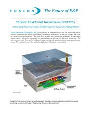
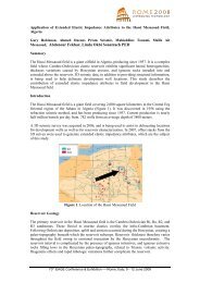
signal. However, the TFCWT spectrum (Figure 4) does not
show any erroneous attenuation. The blurring effect on each
end is because the TFCWT has high-frequency resolution and
low-time resolution at low frequencies and low-frequency resolution
and high time resolution at high frequencies. Thus, the
TFCWT improves resolution for a nonstationary signal. In addition
to the improvement in the time-frequency resolution,
the new methodology inheriting the CWT avoids the subjective
choice of window length necessary for the STFT.
APPLICATIONS OF TFCWT TO FIELD DATA
Time-frequency spectra produced from the TFCWT can be
used to interpret seismic data in the frequency domain. We
have conducted such analyses with poststack data sets. Adding
a frequency axis to a 2D seismic section makes the data
where the scaled and modulated window is given by
−iωτ ˆψ(σω)e ¯ˆψ ω (σ ) = .
C ψ σ 3/2 (13)
Here,
¯ˆψ ω (σ ) is the complex conjugate of ˆψ ω (σ ).
Equation 12 shows that the effective window is the scaled
and modulated wavelet that acts on the transformed signal in
the wavelet domain. In contrast, the chosen window in the
STFT directly operates on the time-domain signal given in
equation 2, and the inner product space is integrated over all
times. The time-frequency map generated by equation 11 or
equation 12 from the scalogram F W (σ, τ) is not obtained by
the direct transformation of a scale to its center frequency;
rather, this map provides energy at the desired frequency and
avoids the complication of overlapping frequency bands common
to a scale-frequency transformation. Equation 11 can be
computed using a two-step procedure. First, we evaluate the
convolution integral in equation 4 to obtain F W (σ, τ) using
the Fourier transform method. In the second step we use the
Fourier transformation of the scaled and modulated wavelet
to compute the inner product over all scales. Note that the
time summation of equation 11 gives the Fourier transform of
the signal. Thus, reconstructing the original signal is a two-step
process: (1) time summation of the TFCWT and (2) inverse
Fourier transform of the resultant sum.
The synthetic signal (Figure 1) is comprised of two hyperbolic
sweep frequencies, each having constant amplitude.
In other words, energy in each frequency sweep is constant
with time. The typical CWT spectrum (Figure 3) for the synthetic
signal improves time-frequency resolution more than
Figure 4. TFCWT spectrum, described by equation 11, obtained
for the chirp signal shown in Figure 1 using a complex
Morlet wavelet.

Time-Frequency Decomposition
P23
three-dimensional. Comparison of single-frequency sections
from such a 3D volume can help detect low-frequency shadows
sometimes caused by hydrocarbon reservoirs. Sun et al.
(2002) use instantaneous spectral analysis based on matchingpursuit
decomposition for direct hydrocarbon detection. A
matching pursuit isolates the signal structures that are coherent
with respect to a given wavelet dictionary (Mallat and
Zhang, 1993). However, if the signal is composed of several
combinations of fundamental dictionaries, it will be difficult to
choose a particular one to analyze the nonstationary nature. In
the TFCWT, time-frequency decomposition is carried out by
a mother wavelet. This method provides good frequency resolution
at low frequencies and is therefore effective in detecting
low-frequency shadows.
A seismic section from a Nigeria data set (Figure 5) shows
bright amplitudes (yellow arrows) adjacent to faults (green arrows),
indicative of known hydrocarbon zones. A preferentially
illuminated single-frequency section at 20 Hz from the
TFCWT data volume shows high-amplitude, low-frequency
Figure 5. A seismic section from a Nigeria data set. Bright
amplitudes indicated by yellow arrows adjacent to the faults
(green arrows) in this seismic section are known hydrocarbon
zones.
anomalies (red) at the reservoir level (yellow arrows) in
Figure 6. Furthermore, at 33 Hz these anomalies disappear
(Figure 7). In this example these low-frequency anomalies appear
only at the known hydrocarbon reservoirs. Mechanisms
for this low-frequency anomaly are not known. Ebrom (2004)
suggests several possible mechanisms of frequency shadow effect.
The challenge is to determine which are first-order effects
and which are less important. The anomaly above the hydrocarbon
reservoir level (black arrow) in the 33-Hz section is
most likely a very thin-bed interference effect that remains
anomalous at higher frequencies. This example shows that
the comparison of single low-frequency sections from TFCWT
has been able to detect low-frequency anomalies caused by
hydrocarbons.
We extend this idea to stratigraphic analysis by observing a
horizon slice from a 3D volume. Adding a frequency axis to a
3D seismic data volume makes the time-frequency volume 4D
and complicates visualization. To simplify visualization, a 3D
seismic data volume can be rearranged in two-dimensions according
to the trace numbers or CDPs. Time-frequency analysis
will extend it in the third dimension, adding a frequency
axis to it. From this time-frequency-CDP volume, we can extract
a horizon or time slice and rearrange the trace numbers
according to their inline and crossline numbers to produce a
frequency-space cube [similar to a tuning cube (Partyka et al.,
1999)]. Visualizing single-frequency attributes for a horizon
from such a 3D cube can be used to identify geologic features
that otherwise would not be visible on a usual horizon amplitude
map. We utilize the fact that the varying thicknesses tune
at varying frequencies. (For details on tuning frequency modeling,
see Marfurt and Kirlin, 2001.)
A horizon slice from the Stratton 3D seismic data volume
is shown in Figure 8b. This horizon slice is taken 16 ms above
the horizon A pick in Figure 8a. A channel, indicated in red,
appears to have branches in the middle of the map toward
the south. From an interpreter’s point of view, knowing the
extension of the possible channel is important information
for reservoir characterization. A 32-Hz frequency slice for the
same horizon slice (Figure 9) shows what could be details of
a fluvial-channel system. We observe a pattern similar to that
Figure 6. A 20-Hz seismic section obtained using TFCWT processing
of the seismic data shown in Figure 5. High-amplitude,
low-frequency anomalies (red) are at the hydrocarbon zones
(yellow arrows).
Figure 7. A 33-Hz seismic section of Figure 5 obtained using
TFCWT processing. In this section frequency anomalies associated
with frequency shadows are absent (yellow arrows).
The anomaly (black arrow) present in this section is from local
tuning effects and does not disappear at higher frequencies.

P24
Sinha et al.
of a complex meandering-channel system in the
southwestern part of the figure. Also note that
the apparent internal heterogeneity of the main
fluvial-channel system is enhanced by spectral
decomposition. The relatively low spectral amplitude
of the channel is indicative of a lithology
change (possibly brine-filled sand).
CONCLUSIONS
Figure 8. (a) A vertical seismic section through the Stratton 3D data set corresponding
to line AB shown in (b). (b) A horizon slice through the seismic
amplitude volume 16 ms above the horizon A pick shown in (a). A fluvial
channel (yellow arrow) shows up as a negative-amplitude trough on the
horizon slice and corresponds to the channel shown in (a). The southwestern
branch of this channel is not clear.
A conventional method of computing a timefrequency
spectrum, or spectrogram, using the
STFT method requires a predefined time window
and therefore has fixed time-frequency
resolution. However, to analyze a nonstationary
signal where frequency changes with time,
we require a time-varying window. The CWT
dilates and compresses wavelets to provide a
time-scale spectrum instead of a time-frequency
spectrum. Converting a scalogram into a timefrequency
spectrum using the center frequency
of a scale gives an erroneous attenuation in the
spectrum. The TFCWT overcomes this problem
and gives a more robust technique of timefrequency
localization. Since TFCWT is fundamentally
derived from the continuous-wavelet
transform, wavelet dilation and compression effectively
provides the optimal window length,
depending upon the frequency content of the signal.
Thus, it eliminates the subjective choice of
a window length and provides an optimal timefrequency
spectrum without any erroneous attenuation
effect for a nonstationary signal. It has
high-frequency resolution at low frequencies and
high time resolution at high frequencies, whereas
the spectrogram has fixed time-frequency resolution
throughout.
Thus, in nonstationary seismic data analysis
the TFCWT has a natural advantage over the
STFT and the typical CWT spectrum. Though
STFT allows one to analyze an entire stratigraphic
interval, TFCWT is focused on the spectral
attributes of horizons rather than intervals.
STFT may be more efficient for estimating the
spectral characteristics of long intervals as compared
to the support of the CWT. However,
TFCWT can be summed over time to resolve the
spectrum of any desired interval. The field examples
on single-frequency sections and maps from
the TFCWT presented in this work suggest that
such analysis potentially can be used as direct
hydrocarbon indicators and for improved stratigraphic
visualization.
ACKNOWLEDGMENTS
Figure 9. A horizon slice at 32 Hz through the TFCWT volume corresponding
to the seismic-amplitude map shown in Figure 8b. Note the channel
extension (blue arrows) and internal heterogeneity of the fluvial-channel
system.
The authors acknowledge the Conoco research
scientists for their valuable input. They
would also like to thank Conoco (now ConocoPhillips)
for providing a field-data set and logistical
support for this research and particularly
Dale Cox of Conoco for many useful discussions

Time-Frequency Decomposition
P25
and help in the practical implementation in SeismicUnix (SU).
The authors are grateful to the Shell Crustal Imaging Facility
at the University of Oklahoma for software support. Finally,
the authors thank Kurt Marfurt, the associate editor of Geophysics,
and two reviewers for their valuable comments and
suggestions.
REFERENCES
Abry, P., P. Goncalves, and P. Flandrin, 1993, Wavelet-based spectral
analysis of 1/f processes: International Conference on Acoustic,
Speech and Signal Processing, IEEE, Proceedings, 3, 237–240.
Castagna, J. P., S. Sun, and R. W. Seigfried, 2003, Instantaneous spectral
analysis: Detection of low-frequency shadows associated with
hydrocarbons: The Leading Edge, 22, 120–127.
Cohen, L., 1995, Time-frequency analysis: Prentice Hall, Inc.
Daubechies, I., 1992, Ten lectures on wavelets: Society of Industrial
and Applied Mathematics.
Dilay, A., and J. Eastwood, 1995, Spectral analysis applied to seismic
monitoring of thermal recovery: The Leading Edge, 14, 1117–1122.
Ebrom, D., 2004, The low frequency gas shadows in seismic sections:
The Leading Edge, 23, 772.
Hardy, H. H., A. B. Richard, and J. D. Gaston, 2003, Frequency estimates
of seismic traces: Geophysics, 68, 370–380.
Hlawatsch, F., and G. F. Boudreaux-Bartels, 1992, Linear and quadratic
time-frequency signal representations: IEEE Signal Processing,
9, no. 2, 21–67.
Jones, D. L., and R. G. Baraniuk, 1995, An adaptive optimal-kernel
time-frequency representation: IEEE Transactions on Signal Processing,
43, 2361–2371.
Mallat, S., 1999, A wavelet tour of signal processing, 2nd ed.: Academic
Press Inc.
Mallat, S., and Z. Zhang, 1993, Matching pursuits with time-frequency
dictionaries: IEEE Transactions on Signal Processing, 41, 3397–
3415.
Marfurt, K. J., and R. L. Kirlin, 2001, Narrow-band spectral analysis
and thin-bed tuning: Geophysics, 66, 1274–1283.
Mitchell, J. T., N. Derzhi, and E. Lickman, 1997, Low frequency shadows:
The rule, or the exception? 67th Annual International Meeting,
SEG, Expanded Abstracts, 685–686.
Partyka, G., J. Gridley, and J. Lopez, 1999, Interpretational applications
of spectral decomposition in reservoir characterization: The
Leading Edge, 18, 353–360.
Peyton, L., R. Bottjer, and G. Partyka, 1998, Interpretation of incised
valleys using new 3-D seismic techniques: A case history using spectral
decomposition and coherency: The Leading Edge, 17, 1294–
1298.
Rioul, O., and M.Vetterli, 1991, Wavelets and signal processing: IEEE
Signal Processing, 8, no. 4, 14–38.
Sinha, S., 2002, Time-frequency localization with wavelet transform
and its application in seismic data analysis: M.S. thesis, University
of Oklahoma.
Sun, S., J. P. Castagna, and R. W. Seigfried, 2002, Examples of wavelet
transform time-frequency analysis in direct hydrocarbon detection:
72nd Annual International Meeting, SEG, Expanded Abstracts,
457–460.
Torrence, C., and G. P. Compo, 1998, A practical guide to wavelet
analysis: Bulletin of the American Meteorological Society, 79,
no. 1, 61–78.