Gauss-Jordan Elimination Method - The Ohio State University

TA: In Kwon Park CRP 762
park.793@osu.edu
Prof. Jean-Michel Guldmann
April 13, 2009
Handout
Gauss-Jordan Elimination Method
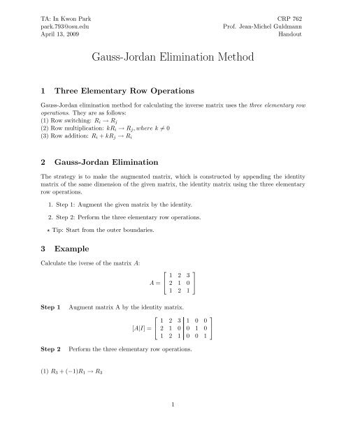
1 Three Elementary Row Operations
Gauss-Jordan elimination method for calculating the inverse matrix uses the three elementary row
operations. They are as follows:
(1) Row switching: R i → R j
(2) Row multiplication: kR i → R j , where k ≠ 0
(3) Row addition: R i + kR j → R i
2 Gauss-Jordan Elimination
The strategy is to make the augmented matrix, which is constructed by appending the identity
matrix of the same dimension of the given matrix, the identity matrix using the three elementary
row operations.
1. Step 1: Augment the given matrix by the identity.
2. Step 2: Perform the three elementary row operations.
⋆ Tip: Start from the outer boundaries.
3 Example
Calculate the iverse of the matrix A:
⎡
A = ⎣
1 2 3
2 1 0
1 2 1
⎤
⎦
Step 1
Step 2
Augment matrix A by the identity matrix.
⎡
1 2 3 1 0
⎤
0
[A|I] = ⎣ 2 1 0 0 1 0 ⎦
1 2 1 0 0 1
Perform the three elementary row operations.
(1) R 3 + (−1)R 1 → R 3
1

Multiply Row 1 by −1, add it to Row 3, and substitute the result for Row 3.
⎡
1 2 3 1 0
⎤
0
⎣ 2 1 0 0 1 0 ⎦
0 0 −2 −1 0 1
(2) − 1 2 R 3 → R 3
Multiply Row 3 by − 1 2
and substitute the result for Row 3.
⎡
⎤
1 2 3 1 0 0
⎣ 2 1 0 0 1 0 ⎦
1
0 0 1
2
0 − 1 2
(3) R 1 + (−3)R 3 → R 1
Multiply Row 3 by −3, add it to Row 1, and substitute the result for Row 1.
⎡
1 2 0 − 1 ⎤
3
2
0
2
⎣ 2 1 0 0 1 0 ⎦
1
0 0 1
2
0 − 1 2
(4) R 2 + (−2)R 1 → R 2
Multiply Row 1 by −1, add it to Row 2, and substitute the result for Row 2.
⎡
1 2 0 − 1 ⎤
3
2
0
2
⎣ 0 −3 0 1 1 −3 ⎦
1
0 0 1
2
0 − 1 2
(5) − 1 3 R 2 → R 2
Multiply Row 2 by − 1 3
, and substitute the result for Row 2.
⎡
1 2 0 − 1 3
2
0
2
⎣ 0 1 0 − 1 3
− 1 3
1
1
0 0 1
2
0 − 1 2
(6) R 1 + (−2)R 2 → R 1
Multiply Row 2 by −2, add it to Row 1, and substitute the result for Row 1.
⎡
⎤
1 2 1
1 0 0
6 3 2
⎣ 0 1 0 − 1 3
− 1 3
1 ⎦
1
0 0 1
2
0 − 1 2
The above matrix is equal to [ I|A −1] , and hence the inverse matrix of A is the right part of the
matrix. That is,
⎡
A −1 = ⎣
1
6
2
3
− 1 2
− 1 3
− 1 3
1
1
2
0 − 1 2
⎤
⎦
⎤
⎦
2