The Atomic Nucleus: a Bound System of ... - Nuclear Physics
The Atomic Nucleus: a Bound System of ... - Nuclear Physics
The Atomic Nucleus: a Bound System of ... - Nuclear Physics

You also want an ePaper? Increase the reach of your titles
YUMPU automatically turns print PDFs into web optimized ePapers that Google loves.
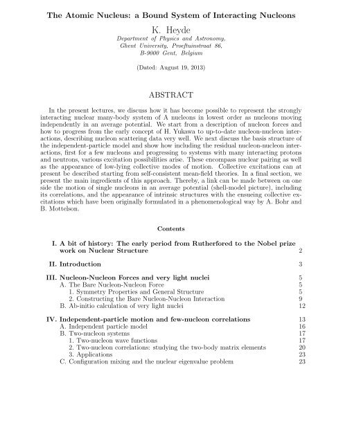
<strong>The</strong> <strong>Atomic</strong> <strong>Nucleus</strong>: a <strong>Bound</strong> <strong>System</strong> <strong>of</strong> Interacting Nucleons<br />
K. Heyde<br />
Department <strong>of</strong> <strong>Physics</strong> and Astronomy,<br />
Ghent University, Proeftuinstraat 86,<br />
B-9000 Gent, Belgium<br />
(Dated: August 19, 2013)<br />
ABSTRACT<br />
In the present lectures, we discuss how it has become possible to represent the strongly<br />
interacting nuclear many-body system <strong>of</strong> A nucleons in lowest order as nucleons moving<br />
independently in an average potential. We start from a description <strong>of</strong> nucleon forces and<br />
how to progress from the early concept <strong>of</strong> H. Yukawa to up-to-date nucleon-nucleon interactions,<br />
describing nucleon scattering data very well. We next discuss the basis structure <strong>of</strong><br />
the independent-particle model and show how including the residual nucleon-nucleon interactions,<br />
first for a few nucleons and progressing to systems with many interacting protons<br />
and neutrons, various excitation possibilities arise. <strong>The</strong>se encompass nuclear pairing as well<br />
as the appearance <strong>of</strong> low-lying collective modes <strong>of</strong> motion. Collective excitations can at<br />
present be described starting from self-consistent mean-field theories. In a final section, we<br />
present the main ingredients <strong>of</strong> this approach. <strong>The</strong>reby, a link can be made between on one<br />
side the motion <strong>of</strong> single nucleons in an average potential (shell-model picture), including<br />
its correlations, and the appearance <strong>of</strong> intrinsic structures with the ensueing collective excitations<br />
which have been originally formulated in a phenomenological way by A. Bohr and<br />
B. Mottelson.<br />
Contents<br />
I. A bit <strong>of</strong> history: <strong>The</strong> early period from Rutherfored to the Nobel prize<br />
work on <strong>Nuclear</strong> Structure 2<br />
II. Introduction 3<br />
III. Nucleon-Nucleon Forces and very light nuclei 5<br />
A. <strong>The</strong> Bare Nucleon-Nucleon Force 5<br />
1. Symmetry Properties and General Structure 5<br />
2. Constructing the Bare Nucleon-Nucleon Interaction 9<br />
B. Ab-initio calculation <strong>of</strong> very light nuclei 12<br />
IV. Independent-particle motion and few-nucleon correlations 13<br />
A. Independent particle model 16<br />
B. Two-nucleon systems 17<br />
1. Two-nucleon wave functions 17<br />
2. Two-nucleon correlations: studying the two-body matrix elements 20<br />
3. Applications 23<br />
C. Configuration mixing and the nuclear eigenvalue problem 23
V. Many-nucleon correlations: interplay <strong>of</strong> shell-model and collective<br />
excitations 26<br />
A. Construction <strong>of</strong> a multi-nucleon basis 26<br />
1. Angular-momentum coupled basis 26<br />
2. m-scheme basis 27<br />
B. Solving the nuclear many-body eigenvalue problem 29<br />
C. Effective nucleon-nucleon interactions 30<br />
1. Microscopic effective interactions 30<br />
2. Phenomenological effective interactions 33<br />
3. Schematic effective interactions 34<br />
D. Collective excitations in the nuclear shell model 35<br />
1. Large-scale shell-model applications 35<br />
2. Collective excitations: coherence and symmetries 36<br />
VI. Mean-field approach 39<br />
VII. Similarities between shell-model and mean-field approaches 43<br />
VIII. Conclusion 44<br />
IX. Acknowledgments 44<br />
References 44<br />
I. A BIT OF HISTORY: THE EARLY PERIOD FROM RUTHERFORED TO<br />
THE NOBEL PRIZE WORK ON NUCLEAR STRUCTURE<br />
In the field <strong>of</strong> nuclear theory, Nobel prizes were rewarded to E.P.J.Wigner, M.Goeppert-<br />
Mayer and J.H.D.Jensen for their discoveries concerning a shell structure in the atomic<br />
nucleus (Nobel prize in 1963), and, to A.Bohr, B.Mottelson and J.Rainwater for discovering<br />
the deep connection between collective motion and single-particle motion in the atomic nucleus<br />
(Nobel prize in 1975). It turns out that those two major discoveries, with the original<br />
papers dating from 1949, and, 1950-1953, have put their mark on the later work and the evolution<br />
<strong>of</strong> our understanding <strong>of</strong> atomic nuclei over the last 60 years with as a major theme,<br />
trying to reconcile collective motion with individual nucleon motion within a mean field,<br />
incorporating residual interactions. In order to do so, nuclear physicists also needed to understand<br />
the nucleon-nucleon interaction as originating from free nucleon-nucleon scattering<br />
as well as their effective interaction inside the atomic nucleus.<br />
Our knowledge <strong>of</strong> the atomic nucleus has mainly been driven by ingenious experimental<br />
work. <strong>The</strong> start came with the α-scattering experiments by Rutherford [1] (1911), experiments<br />
that set the length scale characteristic for the extension <strong>of</strong> the atomic nucleus. Since<br />
then, a number <strong>of</strong> key experiments have disclosed the essential degrees <strong>of</strong> freedom, at the<br />
same time giving rise to an increasing theoretical activity that evolved hand in hand with<br />
the experimental developments.<br />
Let us consider some <strong>of</strong> the very early steps. <strong>The</strong> discovery <strong>of</strong> the neutron by Chadwick<br />
[2](1932) gave rise, within months to the concept <strong>of</strong> charge symmetry using the Pauli spin<br />
matrices and the SU(2) structure proposed by Heisenberg [3]. Experiments providing indications<br />
<strong>of</strong> particular stability for light α-like nuclei were at the origin <strong>of</strong> an extension to<br />
combine isospin and intrinsic spin into the SU(4) Wigner supermultiplet scheme [4], proposing<br />
full charge independence <strong>of</strong> the nucleon-nucleon interaction. <strong>The</strong> latter scheme was at<br />
the origin <strong>of</strong> a first primitive kind <strong>of</strong> nuclear shell model, worked out by Feenberg and Philips<br />
in 1937 [5], using simple forces with exchange character [3, 6, 7] in the 30’s, describing the<br />
2
inding energies from 6 He to 16 O. Discoveries following from radioactive decay studies and<br />
inspecting the abundances <strong>of</strong> the stable elements pointed out the extra stability <strong>of</strong> nuclei that<br />
contained a particular number <strong>of</strong> protons and/or neutrons at 50, 82 and 126, configurations<br />
that posed serious problems to the early shell model. In 1934, Fermi succeeded to perform<br />
nuclear reactions using neutrons, in particular slow ones, thereby covering almost all <strong>of</strong> the<br />
then known stable nuclei (Fermi et al. [8]) and extended the experimental knowledge on<br />
atomic nuclei in a major way. <strong>The</strong>se results resulted in the concept <strong>of</strong> a compound nucleus,<br />
resulting from the strong interactions between protons and neutrons [9] which allowed a<br />
description <strong>of</strong> neutron cross-sections as well as the statistical characteristics at high excitation<br />
energy in the nucleus. <strong>The</strong>se concepts resulted in a new picture <strong>of</strong> the atomic nucleus<br />
to be considered as a charged liquid drop (by Bethe and Bacher [10] and von Weizsäcker<br />
[11] in the mid 30’s) and was at the origin <strong>of</strong> a theoretical description <strong>of</strong> the phenomenon <strong>of</strong><br />
nuclear fission, presented by Bohr and Wheeler [12]. On the other hand, the high precision<br />
obtained in atomic physics studies <strong>of</strong> the hyperfine structure in atoms gave results on magnetic<br />
dipole moments and electric quadrupole moments by Schmidt and Schüler [13, 14] that<br />
pointed towards independent particle motion characterizing the odd nucleon in odd-A nuclei<br />
and the presence <strong>of</strong> an electric quadrupole charge distribution for the nucleus (as shown by<br />
Casimir [15]). A systematic study <strong>of</strong> quadrupole moments by Townes et al., in 1949 [16],<br />
was inconsistent with a single nucleon moving in a central potential indicating the need <strong>of</strong><br />
an induced deformation.<br />
By the end <strong>of</strong> 1940, it was clear that the experimental data were pointing towards two<br />
almost contradictory facets <strong>of</strong> the atomic nucleus: independent particle motion vs. collective<br />
structure. In the field <strong>of</strong> nuclear theory, Nobel prizes were awarded to M. Goepert-Mayer<br />
and J. Hans D. Jensen “for their discoveries concerning nuclear shell studies” [17, 18] and<br />
to A. Bohr, B. Mottelson and J. Rainwater “for the discovery <strong>of</strong> the connection between<br />
collective motion and particle motion in atomic nuclei and the development <strong>of</strong> the theory <strong>of</strong><br />
the structure <strong>of</strong> the atomic nucleus based on this connection” [19–21].<br />
It turned out that those two major steps forward, however, resulted in seemingly conflicting<br />
views with on one side the individual nucleon motion and on the other side collective<br />
degrees <strong>of</strong> freedom. <strong>The</strong>re have been major developments since on a theoretical understanding<br />
<strong>of</strong> both the shell-model and mean-field methods, intimitely connected through underlying<br />
symmetries over a period <strong>of</strong> ∼ 60 years. This would have been impossible without the<br />
enormous developments <strong>of</strong> experimental methods for both the acceleration and detection <strong>of</strong><br />
particles and nuclei, first starting from stable nuclei, later moving away from stability with<br />
the extensive use <strong>of</strong> radioactive beams.<br />
II. INTRODUCTION<br />
Before attempting to start a description <strong>of</strong> the atomic nucleus as a bound system <strong>of</strong><br />
interacting nucleons, it is paramount to learn about the nature <strong>of</strong> the nucleon-nucleon interactions.<br />
We start from the basic properties <strong>of</strong> nucleon-nucleon interactions as manifested<br />
from free nucleon-nucleon scattering. After a short reminder <strong>of</strong> the Schrödinger equation<br />
describing scattering <strong>of</strong> two nucleons through a central potential V(r), we show that the<br />
properties <strong>of</strong> nucleon-nucleon scattering can be described by a set <strong>of</strong> nuclear phase shifts.<br />
We discuss these results for the dominant scattering channels and their importance in understanding<br />
the nucleon-nucleon interaction as a function <strong>of</strong> the collision energy in free space.<br />
<strong>The</strong> next step is to derive an analytical form describing the experimental scattering data. We<br />
are able to constrain the most general form using general invariance properties from quantum<br />
mechanics which the nucleon-nucleon interaction should obey. We stress in particular the<br />
importance <strong>of</strong> a tensor term, which is related to the Yukawa picture using one-pion exchange<br />
as one <strong>of</strong> the decisive elements describing nucleon-nucleon forces, as well as the need <strong>of</strong> a<br />
spin-orbit term. We present an example <strong>of</strong> one <strong>of</strong> the early realistic nucleon-nucleon forces<br />
3
(meaning the force is able to describe nuclear phase shifts up to E lab ∼ 400 MeV) as well<br />
as the more recent Argonne potentials. <strong>The</strong>se nucleon-nucleon forces describe the extensive<br />
experimental data set <strong>of</strong> nucleon-nucleon phase shifts extremely well as will be illustrated.<br />
Moving to very recent work, it is shown that the most important central components <strong>of</strong> the<br />
free nucleon-nucleon interaction can be derived from lattice QCD calculations.<br />
Attempting to describe the very light nuclei such as 3 H and 3 He starting from realistic<br />
nucleon-nucleon interactions, however, leads to underbound nuclei. This shows the need <strong>of</strong><br />
introducing three-nucleon interaction terms which is illustrated for the nuclei up to mass<br />
number A=12 ( 12 C), indicating the need <strong>of</strong> both two-nucleon and three-nucleon terms to<br />
describe these very light nuclei from ab-initio calculations. We close by facing the problems<br />
that arise when trying to use these realistic interactions in order to describe the effective<br />
interactions inside the nucleus, containing many interacting protons and neutrons.<br />
<strong>The</strong> stability <strong>of</strong> nuclei and abundances <strong>of</strong> the elements (BE(A) ∼ A), as well as early<br />
experimental data on nuclear ground-state spins and magnetic moments in many odd-mass<br />
nuclei were all pointing towards the existence <strong>of</strong> a central potential in which nucleons move,<br />
to a large extent, as independent particles. In a first part we discuss the concept <strong>of</strong> an<br />
independent-particle model, showing that a harmonic oscillator potential enlarged with a<br />
centrifugal l.l and spin-orbit l.s term, is able to describe consistently the proton and neutron<br />
numbers corresponding to nuclei with increased stability. We go on showing in some detail<br />
the salient features <strong>of</strong> the shell-model structure (single-particle energy spectra and wave<br />
functions, the shell-gaps in the spectra,...).<br />
We then discuss nuclei containing two nucleons outside <strong>of</strong> a closed-shell system and<br />
analyze the energy correction that results from the interaction between these two “valence”<br />
nucleons. In order to obtain quantitative results, we start from simple central forces to<br />
derive the interaction energy, splitting the degeneracy <strong>of</strong> the two-nucleon system. A generic<br />
property shows up, i.e., the two nucleons (protons or neutrons) preferentially pair up in a<br />
state <strong>of</strong> angular momentum J = 0. We illustrate this important result with examples such as<br />
the separation energy <strong>of</strong> a nucleon from a given nucleus as well as analyzing energy spectra<br />
<strong>of</strong> nuclei with two nucleons outside (or missing) <strong>of</strong> a closed-shell core.<br />
We move on to make the simple analyses, in which the two nucleons are constrained to one<br />
single-particle orbital, more realistic. In general, the two nucleons can occupy more singleparticle<br />
states and consequently give rise to a number <strong>of</strong> possible configurations, forming a<br />
quantum mechanical basis to solve the nuclear energy eigenvalue problem, starting from a<br />
given two-body interaction. We present, in detail, the procedure for a simple nucleus 18 O,<br />
in which the two valence nucleons can move in the N=2 (1d 5/2 , 2s 1/2 , 1d 3/2 ) orbitals. We<br />
discuss the results in the case <strong>of</strong> 18 0 and 210 Po, pointing out the presence <strong>of</strong> a generic pairing<br />
results that two-nucleon correlations exhibit throughout the nuclear mass table.<br />
Starting from the detailed discussion for two-nucleon systems, we generalize the nuclear<br />
energy eigenvalue problem to systems with a large number <strong>of</strong> active protons and/or neutrons<br />
moving in a given model space (configuration space). To do so we discuss (i) how to<br />
build a basis needed to expand the full wave function, emphasizing the rapid increase in<br />
dimension <strong>of</strong> the eigenvalue problem and the corresponding computational issues, and, (ii)<br />
how to handle the nucleon-nucleon interaction acting inside the atomic nucleus. <strong>The</strong> latter<br />
point needs particular attention since one can (i) start from relatively simple schematic interactions<br />
(putting forward an analytical form), (ii) start from the nuclear two-body matrix<br />
elements, called the empirical effective interaction, which are used as parameters that are<br />
fixed by fitting the calculated observables (energy, lifetimes in γ- and β,..) to a large set<br />
<strong>of</strong> the corresponding nuclear data in a given region <strong>of</strong> the nuclear mass table, or, (iii) start<br />
from a realistic interaction, however, adapting this force for use inside an atomic nucleus<br />
constructing the nuclear G-matrix.<br />
We subsequently go through the various steps in order to apply the nuclear shell model<br />
for the rather complex systems <strong>of</strong> many interacting nucleons (encompassing both protons<br />
4
and/or neutrons). We illustrate the advances that have been made from the early 1p-shell<br />
nuclei (1965) towards recent calculations with very big model spaces and many nucleons. In<br />
particular we show results for the sd shell and the fp shell. In the latter case, it is shown<br />
that structures reminiscent <strong>of</strong> collective modes <strong>of</strong> motion (macroscopic) appear. We make<br />
a side-step to show what may be the deeper origin <strong>of</strong> such collective modes resulting from a<br />
purely microscopic shell-model approach.<br />
Finally, we consider nuclei with a single closed shell, such as the N=126 isotones and<br />
the Sn isotopes. We point out that the characteristic energy spectra resulting from the<br />
shell-model calculations can be understood from an unexpected point <strong>of</strong> view, emphasizing<br />
symmetries connected to the formation <strong>of</strong> nucleon pairs in long series <strong>of</strong> isotones (isotopes).<br />
III. NUCLEON-NUCLEON FORCES AND VERY LIGHT NUCLEI<br />
Since our basic assumption in using the shell-model to approximate the complicated<br />
nuclear many-body problem <strong>of</strong> A nucleons interacting inside the atomic nucleus is the use<br />
<strong>of</strong> an effective ‘in-medium’ interaction, we will start by giving some general discussion <strong>of</strong><br />
those forces used throughout the present lectures.<br />
It is standard to determine a general form by imposing certain symmetry constraints (see<br />
further in the text), and the strength <strong>of</strong> this general form is fitted to experimental data<br />
describing free nucleon-nucleon scattering up to ≃ 350 MeV laboratory energy [22].<br />
A. <strong>The</strong> Bare Nucleon-Nucleon Force<br />
<strong>The</strong> bare nucleon-nucleon force describes the interaction between two free nucleons (see<br />
Figure 1). It is understood that the effect <strong>of</strong> the Coulomb-interaction is treated separately,<br />
so we focus entirely on the effect <strong>of</strong> the strong interaction between the nucleons.<br />
<strong>The</strong> derivation <strong>of</strong> the interaction between free nucleons is based on some important assumptions<br />
[23]:<br />
- we consider no substructure in the nucleon, and consider nucleons to describe the<br />
essential degrees <strong>of</strong> freedom,<br />
- the A nucleons interact via a potential,<br />
- relativistic effects are negligible,<br />
- only two-body forces are considered.<br />
<strong>The</strong> first assumption states that the interaction between two nucleons goes via a potential.<br />
<strong>The</strong> potential depends only on those two nucleons, and the dependence on their coordinates<br />
can be expressed in the most general way as:<br />
V (1, 2) = V (⃗r 1 , ⃗p 1 ,⃗σ 1 ,⃗τ 1 ,⃗r 2 , ⃗p 2 ,⃗σ 2 ,⃗τ 2 ), (1)<br />
where ⃗r i denotes the spatial coordinate <strong>of</strong> nucleon i = 1, 2; ⃗p i the momentum; ⃗σ i the spin,<br />
and ⃗τ i the isospin coordinates.<br />
1. Symmetry Properties and General Structure<br />
<strong>The</strong> potential V (1, 2) has to fulfil a number <strong>of</strong> symmetry properties, imposed by the<br />
nature <strong>of</strong> the strong interaction between free nucleons:<br />
5
• hermiticity<br />
• invariance under an exchange <strong>of</strong> the coordinates<br />
• translational invariance<br />
with ⃗r = ⃗r 1 − ⃗r 2 the relative spatial coordinate.<br />
• Galilean invariance<br />
with ⃗p = 1 2 (⃗p 1 − ⃗p 2 ) the relative momentum.<br />
V (1, 2) = V (2, 1). (2)<br />
V (1, 2) = V (⃗r, ⃗p 1 ,⃗σ 1 ,⃗τ 1 , ⃗p 2 ,⃗σ 2 ,⃗τ 2 ), (3)<br />
V (1, 2) = V (⃗r, ⃗p,⃗σ 1 ,⃗τ 1 ,⃗σ 2 ,⃗τ 2 ), (4)<br />
• invariance under space reflection (parity conservation)<br />
• invariance under time reversal<br />
V (⃗r, ⃗p,⃗σ 1 ,⃗τ 1 ,⃗σ 2 ,⃗τ 2 ) = V (−⃗r, −⃗p,⃗σ 1 ,⃗τ 1 ,⃗σ 2 ,⃗τ 2 ). (5)<br />
V (⃗r, ⃗p,⃗σ 1 ,⃗τ 1 ,⃗σ 2 ,⃗τ 2 ) = V (⃗r, −⃗p, −⃗σ 1 ,⃗τ 1 , −⃗σ 2 ,⃗τ 2 ). (6)<br />
• rotational invariance in coordinate space<br />
Also introducing the orbital angular momentum ⃗ L = ⃗r × ⃗p, only terms <strong>of</strong> the form<br />
⃗σ 1 · ⃗σ 2 , (⃗r · ⃗σ 1 )(⃗r · ⃗σ 2 ), (⃗p · ⃗σ 1 )(⃗p · ⃗σ 2 ), ( ⃗ L · ⃗σ 1 )( ⃗ L · ⃗σ 2 ) + ( ⃗ L · ⃗σ 2 )( ⃗ L · ⃗σ 1 ) are possible.<br />
Multiplication with an arbitrary function <strong>of</strong> r 2 , p 2 and ⃗ L · ⃗L does not affect this<br />
symmetry constraint.<br />
• rotational invariance in isospin space<br />
Only terms <strong>of</strong> the form:<br />
V 0 + V τ ⃗τ 1 · ⃗τ 2 , (7)<br />
are allowed.<br />
A more elaborate discussion <strong>of</strong> the symmetry properties is given by Ring and Schuck [23].<br />
One can make several combinations with good symmetry, but we present those combinations<br />
that have been used mainly in order to construct a realistic bare two-body nucleon<br />
interaction.<br />
a. Central Force Component <strong>The</strong> central forces are local forces since they do not depend<br />
on the velocity, and contain only scalar products <strong>of</strong> the major nucleon variables ⃗σ and<br />
⃗τ:<br />
V C (1, 2) = V 0 (r) + V σ (r)⃗σ 1 · ⃗σ 2 + V τ (r)⃗τ 1 · ⃗τ 2 + V στ (r)⃗σ 1 · ⃗σ 2 ⃗τ 1 · ⃗τ 2 . (8)<br />
This form can be rewritten using certain exchange operators. One defines the spin exchange<br />
operator ̂P σ :<br />
̂P σ = 1 2 (1 + ⃗σ 1 · ⃗σ 2 ), (9)<br />
and, likewise, the isospin exchange operator ̂P τ :<br />
̂P τ = 1 2 (1 + ⃗τ 1 · ⃗τ 2 ). (10)<br />
6
<strong>The</strong> expectation value <strong>of</strong> ̂P σ becomes:<br />
〈SM S | ̂P σ |SM S 〉 = 〈SM S | 1 2<br />
= S(S + 1) − 1<br />
=<br />
{<br />
1 for S = 1<br />
−1 for S = 0.<br />
(<br />
1 + 2( S ⃗ )<br />
2 − ⃗s 1 2 − ⃗s 2 2 ) |SM S 〉<br />
(11)<br />
If ̂P σ would act on a two-particle state with spin S = 1 (spin-triplet state or spin-symmetric<br />
state), there is no change <strong>of</strong> sign for the spin wave function; if it would act on a S = 0 state<br />
(spin-singlet or spin-antisymmetric), it produces an extra minus sign, to be interpreted as the<br />
interchange <strong>of</strong> the individual spin coordinates. Similar relations hold for ̂P τ . <strong>The</strong> exchange<br />
operator ̂P r for the spatial coordinate can be defined through the relation:<br />
̂P r ̂P<br />
σ ̂P τ = −1, (12)<br />
since the wave function has to be antisymmetric under the interchange <strong>of</strong> all coordinates <strong>of</strong><br />
particles 1 and 2. Using (12), ̂P τ can be rewritten as:<br />
and the general central force becomes:<br />
̂P τ = − ̂P r ̂P σ , (13)<br />
V C = V W (r) + V M (r) ̂P r + V B (r) ̂P σ + V H (r) ̂P r ̂P σ . (14)<br />
<strong>The</strong> coefficients <strong>of</strong> the different terms in (8) and (14) fulfil the following relation:<br />
V W = V 0 − V σ − V τ + V στ , (Wigner force) (15)<br />
V M = −4V στ , (Majorana force) (16)<br />
V B = 2V σ − 2V στ , (Bartlett force) (17)<br />
V H = −2V τ + 2V στ .(Heisenberg force) (18)<br />
Yet another way <strong>of</strong> writing down the central interaction makes use <strong>of</strong> projection operators:<br />
̂Π σ s = 1 2 (1 − ̂P σ ) , ̂Πσ t = 1 2 (1 + ̂P σ ), (19)<br />
̂Π r o = 1 2 (1 − ̂P r ) , ̂Πr e = 1 2 (1 + ̂P r ). (20)<br />
Since table I indicates that it is sufficient to know the spin and isospin symmetry in order<br />
to establish the correct antisymmetry <strong>of</strong> the wave function, one can write the central force<br />
in terms <strong>of</strong> the operators iĵΠ, defined as:<br />
iĵΠ ≡<br />
(2T+1)(2S+1)̂Π ≡<br />
2T+1̂Π2S+1̂Π, (21)<br />
1<br />
[ ]<br />
2T+1̂Π = 1 − (−1) T τ ̂P , (22)<br />
2<br />
1<br />
[ ]<br />
2S+1̂Π = 1 − (−1) S σ ̂P . (23)<br />
2<br />
<strong>The</strong> expression for the central force then becomes:<br />
∑<br />
V C = V C (r) a ij<br />
iĵΠ. (24)<br />
i,j={1,3}<br />
<strong>The</strong> relationship between the various representations <strong>of</strong> the central force is summarized in<br />
table II.<br />
7
TABLE I: Different combinations giving rise to a totally antisymmetric two-body nuclear wave<br />
function. <strong>The</strong> notation 〈⃗σ 1 · ⃗σ 2 〉 is a shorthand notation for the expectation value <strong>of</strong> the operator<br />
in a given two-particle state with total spin S: 〈( 1 1<br />
2 2 )SM S|⃗σ 1 · ⃗σ 2 |( 1 1<br />
2 2 )SM S〉. Likewise, 〈⃗τ 1 · ⃗τ 2 〉 is<br />
a shorthand notation for 〈( 1 1<br />
2 2 )TT z|⃗τ 1 · ⃗τ 2 |( 1 1<br />
2 2 )TT z〉.<br />
〈⃗σ 1 · ⃗σ 2 〉 〈⃗τ 1 · ⃗τ 2 〉 S T spatial<br />
-3 -3 0 0 odd<br />
-3 1 0 1 even<br />
1 -3 1 0 even<br />
1 1 1 1 odd<br />
TABLE II: Relation between the coefficients <strong>of</strong> the various representations (equations (8), (14) and<br />
(24)) <strong>of</strong> the central force.<br />
〈⃗σ 1 · ⃗σ 2 〉 〈⃗τ 1 · ⃗τ 2 〉 V (⃗σ 1 · ⃗σ 2 ,⃗τ 1 · ⃗τ 2 ) V ( ̂P r , ̂P σ )<br />
ij ̂Π<br />
1 -3 V 0 + V σ − 3V τ − 3V στ V W + V M + V B + V H a 13<br />
-3 1 V 0 − 3V σ + V τ − 3V στ V W + V M − V B − V H a 31<br />
1 1 V 0 + V σ + V τ + V στ V W − V M + V B − V H a 33<br />
-3 -3 V 0 − 3V σ − 3V τ + 9V στ V W − V M − V B + V H a 11<br />
b. Two-Body Tensor Force Component <strong>The</strong> two-body tensor force also has a local<br />
character, and has the form:<br />
( )<br />
3(⃗σ1 · ⃗r)(⃗σ 2 · ⃗r)<br />
V T (1, 2) = V T (r) (v t0 + v tt ⃗τ 1 · ⃗τ 2 )<br />
− ⃗σ<br />
r 2 1 · ⃗σ 2 (25)<br />
V T (1, 2) = V T (r) (v t0 + v tt ⃗τ 1 · ⃗τ 2 ) S 12 , (26)<br />
and S 12 is the tensor operator defined in expression (25). <strong>The</strong> tensor force is particularly<br />
important since it causes orbital angular momentum mixing. Its presence in the nuclear<br />
force is shown by the non-vanishing quadrupole moment <strong>of</strong> the deuteron, which cannot be<br />
proven by a pure central forces alone [23].<br />
c. Two-Body Spin-Orbit Force Component <strong>The</strong> two-body spin-orbit force has a nonlocal<br />
structure:<br />
V lS (1, 2) = V lS (r) ⃗ l · ⃗S, (27)<br />
with ⃗ S the total spin <strong>of</strong> the two-body system, and ⃗ l the relative orbital angular momentum<br />
operator for the two-body system. <strong>The</strong> velocity dependence, or non-local character, enters<br />
the expression through the orbital angular momentum.<br />
d. Radial Dependence <strong>The</strong> radial dependence <strong>of</strong> the various contributions can be parameterized<br />
using simple central potentials. Various forms are <strong>of</strong>ten used:<br />
Yukawa potential: V (r) = −V 0<br />
e −µr<br />
µr ,<br />
Gaussian potential: V (r) = −V 0 e −r2 /r 2 0 ,<br />
exponential potential: V (r) = −V 0 e −r/r 0<br />
,<br />
square well: V (r) = −V 0 if r ≤ r 0<br />
V (r) = 0 if r > r 0 .<br />
<strong>The</strong> strength V 0 and range r 0 are fitted to the experimental data.<br />
8
<strong>The</strong> Yukawa potential [24], however, is based on field theory: the long-distance attractive<br />
tail <strong>of</strong> the nuclear force is mediated by the exchange <strong>of</strong> one pion between the interacting<br />
nucleons. <strong>The</strong> simplest form is derived from the exchange <strong>of</strong> a single pion. In this case,<br />
1/µ = ¯h/m π c is the Compton wavelength <strong>of</strong> the pion, and is given by µ = 0.70 fm −1 .<br />
Although the effective nucleon-nucleon interaction (active in some limited part <strong>of</strong> the full<br />
Hilbert space and within a nuclear medium) will be largely different from the form <strong>of</strong> the<br />
free nucleon-nucleon interaction [22], we will start considering the properties <strong>of</strong> the bare<br />
force. To a good approximation, and incorporating one-pion exchange (OPEP), this latter<br />
force leads to a form <strong>of</strong> the type [24, 25]:<br />
π = 1 f 2 {<br />
3 ¯hc m πc 2 ⃗σ 1 · ⃗σ 2 +<br />
V OPEP<br />
(<br />
1 + 3 µr + 3<br />
(µr) 2 )<br />
S 12<br />
} e<br />
−µr<br />
µr (⃗τ 1 · ⃗τ 2 ), (28)<br />
with c the speed <strong>of</strong> light, m π the pion mass, µ ≡ mπc = 0.70 fm −1 the reduced pion mass,<br />
¯h<br />
and f2<br />
= 0.081 ± 0.002 the pion-nucleon coupling constant. <strong>The</strong> factor S ¯hc 12:<br />
S 12 = 3 (⃗σ 1 · ⃗r)(⃗σ 2 · ⃗r)<br />
r 2 − ⃗σ 1 · ⃗σ 2 , (29)<br />
is the tensor operator. Expression (28) holds typically for a separation distance r = |⃗r 1 −⃗r 2 | ≃<br />
1.5 – 2 fm, but the actual interaction becomes repulsive (in coordinate space) at distances<br />
r ≤ 0.5 fm.<br />
2. Constructing the Bare Nucleon-Nucleon Interaction<br />
Once a general analytical functional form <strong>of</strong> the two-body potential has been laid out, the<br />
parameters <strong>of</strong> the various contributions have to be determined. One can accomplish this by<br />
analyzing the scattering properties in the various two-body nucleon-nucleon systems, as well<br />
as the proton-neutron bound state, i.e. the deuteron. Scattering experiments are performed<br />
below the pion-production threshold (∼ 350 MeV). This guarantees the appropriateness <strong>of</strong><br />
the non-relativistic approach, and the nucleons involved can be treated as point-like particles<br />
(justifying the assumed existence <strong>of</strong> a potential). (see Figure 1).<br />
<strong>The</strong> problem <strong>of</strong> potential scattering between two nucleons can be described by the 2-<br />
particle Schrödinger equation<br />
[− ¯h2<br />
2m 1<br />
∆ 1 − ¯h2<br />
2m 1<br />
∆ 2 + V (1, 2)]ψ(1, 2) = Eψ(1, 2). (30)<br />
Separation in the relative and centre-<strong>of</strong>-mass coordinates is possible, for radial potentials<br />
depending on the relative coordinate r only (⃗r = ⃗r 1 − ⃗r 2 ) and R=1/2(⃗r 1 + ⃗r 2 ), leads to the<br />
Schrödinger equation<br />
[− ¯h2<br />
2m r<br />
∆ r + V (r)]ψ(r) = Eψ(r), (31)<br />
An asymptotic solution (with V(r )→ 0 for short-range potentials) can be written as<br />
ψ + k (r) = ei⃗ k.⃗r + f(θ, φ) eikr<br />
r , (32)<br />
describing the superposition <strong>of</strong> a plane wave solution and an outgoing spherical wave, describing<br />
the scattering process.<br />
<strong>The</strong> plane wave can be expanded in its different partial waves as<br />
9
REACTION CHANNELS<br />
V(1,2)<br />
N<br />
N<br />
S=1, 0 : TRIPLET, SINGLET SPIN STATE<br />
pp, pn and nn scattering states<br />
: even, odd relative angular monentum states<br />
CHARACTERIZED BY ( ,S) J<br />
PHASE SHIFTS IN SCATTERING PROCESS<br />
FIG. 1: Scattering free nucleons.<br />
∞∑<br />
i l (2l + 1)j l (kr)P l (cosθ), (33)<br />
l=0<br />
and the radial form j l (kr) in the asymptotic region can be expressed as<br />
j l (kr) r→∞ ∝ 1<br />
i<br />
− e i(kr−lπ/2)<br />
sin(kr − lπ/2) =<br />
kr 2k [e−i(kr−lπ/2) ]. (34)<br />
r<br />
In the asymptotic form <strong>of</strong> the solution ψ + k<br />
(r), an outgoing spherical wave is present too.<br />
Thus, the radial part in each <strong>of</strong> the partial waves can be expressed as<br />
ψ + k (r) r→∞ ∝ i<br />
2k e−δ l(k) [ e−i(kr−lπ/2) − S l (k)e i(kr−lπ/2)<br />
], (35)<br />
r<br />
with S l (k) = e 2iδl(k) .<br />
In the more realistic cases <strong>of</strong> nucleon-nucleon scattering, the above equations are more<br />
complicated because the interaction V(1,2) as described in section II.A will, in general<br />
depend on the spin state <strong>of</strong> the two nucleons which can be in an S=1 or S=0 state and the<br />
orientation <strong>of</strong> the total spin with respect to the relative angular momentum l (expressed<br />
by the angular momentum coupling ( ⃗ l, S)J) ⃗ as well as on the charge <strong>of</strong> the nucleons, i.e.,<br />
distinguishing nn,pp and np scattering (also expressed by the isospin T quantum number).<br />
Because <strong>of</strong> the presence <strong>of</strong> the tensor force, which can couple relative angular momenta<br />
differing by 2 units, the Schrödinger equations for different values <strong>of</strong> l, i.e., l=0 and l=2,<br />
become coupled. <strong>The</strong> phase shifts are now given by δ(l, S)J(k). <strong>The</strong> general form <strong>of</strong> the<br />
two-nucleon interaction V(1,2) is used to calculate the theoretical phase shifts that are fitted<br />
to the experimental data-basis <strong>of</strong> experimentally deduced phase shifts using a least-squares<br />
method, minimizing ∑ n<br />
i<br />
| δ th (l, S)J −δ exp (l, S)J | 2 . <strong>The</strong>se data are given by a set <strong>of</strong> numbers<br />
10
FIG. 2: <strong>The</strong> nuclear phase parameters for the T = 1 channels with L ≤ 2, up to a laboratory<br />
energy <strong>of</strong> E lab = 400 MeV. <strong>The</strong> phase shifts are given in radians. Positive phase shifts indicate<br />
attraction between the nucleons, negative phase shifts repulsion. Figure taken from [25].<br />
(phase shift expressed in radians) as a function <strong>of</strong> the laboratory scattering energy E lab given<br />
in the notation 2S+1 l J <strong>of</strong> which an example is shown in Figure 2 and contain the information<br />
about the shape, the strength and the energy dependence <strong>of</strong> the potential.<br />
<strong>The</strong>re exist a number <strong>of</strong> potentials that are fitted to nucleon-nucleon scattering data<br />
and the deuteron binding energy. Some <strong>of</strong> the most famous are listed here: the Hamada-<br />
Johnston potential (which is presented in Figure 3) [26, 27], the Reid s<strong>of</strong>t-core potential<br />
[28], the Tabakin potential [29], the Nijmegen potential [30], the Paris potential [31, 32], the<br />
Bonn potential [33, 34], and the modern CD-Bonn, [35], Nijmegen I + II, Reid93 [36] and<br />
the Argonne potentials [37, 38].<br />
<strong>The</strong> Argonne potential consists <strong>of</strong> 8 (or 18) terms:<br />
V ij =<br />
∑<br />
v p (r ij )O p ij , (36)<br />
p=1,8(18)<br />
with the operators O p ij<br />
given by:<br />
O p ij = {1,⃗σ i · ⃗σ j , ⃗ S ij , ⃗ l · ⃗S, . . .} ⊗ {1,⃗τ i · ⃗τ j }. (37)<br />
<strong>The</strong> potentials have been fitted to 4300 nucleon-nucleon scattering data, and describe the<br />
bare scattering process very well over the energy range (up to 350 MeV laboratory scattering<br />
energy) [39]. <strong>The</strong>y are phenomenological but describe the essential physics: Coulomb forces,<br />
one-pion exchange at the larger nuclear separation distance (r ≃ 1.5 – 2 fm), but also the<br />
intermediate and short-range parts.<br />
<strong>The</strong> more data are included, the better the agreement; so it is crucial to fit to protonproton,<br />
neutron-neutron, proton-neutron and deuteron data. Potentials that lack one <strong>of</strong><br />
these sets in their parameter fit, provide a worse description for that particular set, as<br />
demonstrated in [40] for various potential models applied to the proton-proton scattering<br />
data.<br />
11
FIG. 3: Phenomenological central nucleon-nucleon potential V C as obtained from the analysis <strong>of</strong><br />
Hamada and Johnston [26]. <strong>The</strong> dotted potentials correspond to the one-pion exchange potential<br />
(OPEP) <strong>of</strong> expression (28). Figure taken from [25].<br />
Even though these potentials provide a precise description <strong>of</strong> the free nucleon-nucleon<br />
scattering, they are still subject to corrections when proceeding towards light nuclei. Usually,<br />
the potentials fitted to scattering data tend to underbind light nuclei. <strong>The</strong> correct binding<br />
energy is expected to be found by adding three-nucleon forces [39, 41–44].<br />
An approach different from the ones mentioned above involves writing the nucleon-nucleon<br />
potential as a sum over one-boson exchange potentials [45–52].<br />
Moreover, the inclusion <strong>of</strong> relativistic effects may prove to be important too: given the<br />
rather small distance scales, it might be necessary to go beyond the meson picture and<br />
to include quark-antiquark pair exchange, as depicted in Figure 4. However, calculations<br />
become intractable because <strong>of</strong> the strong coupling α s that is too large to allow a perturbative<br />
approach [53].<br />
A review on the present understanding <strong>of</strong> nuclear forces can be found in [54].<br />
B. Ab-initio calculation <strong>of</strong> very light nuclei<br />
At this point, one may ask the question if one could not start from ab-initio methods and<br />
start for the lightest nuclei, using a Hamiltonian containing both 2- and 3-body terms such<br />
as<br />
12
FIG. 4: (a) Representation <strong>of</strong> quark exchange between nucleons via the exchange <strong>of</strong> a quarkantiquark<br />
pair. Antiquarks are depicted as quarks moving backwards in time. (b) <strong>The</strong> exchange<br />
<strong>of</strong> a meson is rather similar to this. Figure taken from [53].<br />
H =<br />
A∑<br />
T i + ∑ V i,j + ∑<br />
V i,j,k . (38)<br />
i i
-20<br />
Energy (MeV)<br />
-25<br />
-30<br />
-35<br />
-40<br />
-45<br />
-50<br />
0 +<br />
4 He<br />
6 He<br />
2 +<br />
0 + 6 Li3 +<br />
1 + 5/2-<br />
7/2-<br />
1/2 -<br />
v 18<br />
IL2T Exp<br />
2+<br />
0+<br />
8 He<br />
7<br />
3/2 -<br />
Li<br />
8 Li<br />
4 + 3 + 10 He<br />
3 +<br />
1 +<br />
1 +<br />
2 + 2 +<br />
0 +<br />
-55<br />
-60<br />
Argonne v18<br />
With Illinois Vijk<br />
0 +<br />
8 Be<br />
3/2 -<br />
9 Li<br />
5/2 -<br />
9 Be<br />
3/2 - 0 + 3 +<br />
-65<br />
GFMC Calculations<br />
10 Be 10 B<br />
-70<br />
FIG. 5: Energy levels for the light nuclei using a Quantum Monte Carlo (QMC) calculation using<br />
2-and 3-body forces [42].<br />
when studying an oscillator under the influence <strong>of</strong> an external, time-varying force field. So,<br />
whenever we like to find out how something sits together, one can either shake it vigorously<br />
and “listen” how the system “responds” or either take it apart into its components. <strong>The</strong>se<br />
two avenues have been taken by<br />
(i) studying the response <strong>of</strong> the atomic nucleus when being probed by external fiels (electromagnetic,<br />
weak and strong probes),<br />
(ii) studying the ways in which unstable nuclei decay and emit particles or photons in<br />
their way back to stability.<br />
<strong>The</strong>se two principles have been used to disclose some <strong>of</strong> the essential degrees <strong>of</strong> freedom<br />
that are active inside the nucleus by studying the various “eigen”-frequencies on which the<br />
nuclear many-body system resonates (see Figure 6).<br />
In this spirit, besides the discovery <strong>of</strong> the various decay modes that have given deep<br />
insight in the way particles or groups <strong>of</strong> particles can be emitted from an unstable nucleus,<br />
a number <strong>of</strong> external probes have been used extensively [57].<br />
a. Scattering experiments using electrons, protons, α-particles, ... gave rise to the notion<br />
<strong>of</strong> an average charge and mass field with a pr<strong>of</strong>ile that resembles very well a liquid<br />
drop <strong>of</strong> charged matter. Moreover, using those probes in ingenious ways, one has been<br />
able to map out the motion <strong>of</strong> nucleons in well-defined single-particle orbitals, much<br />
like in a Bohr atom, even studying the velocity distribution <strong>of</strong> nucleons moving inside<br />
the atomic nucleus and thereby learning on the effective nucleon-nucleon forces that<br />
act at the very short length scale <strong>of</strong> nucleon separation.<br />
b. <strong>Nuclear</strong> reactions in which one, or more nucleons are transferred into a nucleus or<br />
taken out <strong>of</strong> a nucleus: so-called transfer reactions. Those reactions have unambigously<br />
14
CROSS-SECTION (A.U.)<br />
4<br />
3<br />
2<br />
1<br />
Elastic<br />
e -<br />
e -<br />
(hq, h )<br />
photon<br />
Quasi-elastic<br />
Nucleon<br />
<br />
Nucleon<br />
Delta-resonance<br />
0 100 300<br />
h (MeV)<br />
FIG. 6: Schematic cross-section for electron scattering <strong>of</strong>f a nucleus as a function <strong>of</strong> the energy<br />
transfer ¯hω ( in MeV). Different energy regions are highlighted [57].<br />
shown the organization <strong>of</strong> nucleons to move in shell-model orbitals in which nucleons<br />
like to combine into pairs, much like electrons do in the superconducting state in solidstate<br />
physics. This effect has been most clearly shown studying the mass dependence<br />
<strong>of</strong> proton and/or neutron separation energies throughout the nuclear mass table as<br />
well as from the energy spacing between the 0 + ground-state and the first excited 2 +<br />
state in even-even nuclei.<br />
c. Using the disturbance created by a rapidly moving charged particle (or nucleus) when<br />
passing the atomic nucleus. <strong>The</strong> nucleus becomes excited and the internal charge<br />
and magnetic structure can be probed in fine detail. Such reactions showed, e.g.,<br />
the quadrupole reduced transition probabilities for heavy nuclei. <strong>The</strong>se data are a<br />
direct measure <strong>of</strong> the coherence between individual nucleons moving inside the atomic<br />
nucleus and present a most interesting variation with mass number A. So one notices<br />
that the nucleus can sustain various collective modes, much like a charged drop can<br />
vibrate in various modes, rotate,..<br />
d. External probing can also be done using heavy nuclei that come to grazing with a target<br />
nucleus to which a fragment may be transferred but also a lot <strong>of</strong> angular momentum.<br />
In this way, the behavior <strong>of</strong> very regular bands could be formed up to high spin and<br />
excitation energy. Data taken within the early experiments showed the existence <strong>of</strong><br />
superdeformed rotational motion in 152 Dy as discoverd in 1986 by Twin and co-workers<br />
[58]. <strong>The</strong> extensive use <strong>of</strong> state-<strong>of</strong>-the-art gamma-arrays in recent years has given rise<br />
to detailed mapping <strong>of</strong> nuclear excited properties at very high rotation frequencies.<br />
<strong>The</strong> essential point here is that ingenious experimentation using - for each time span,<br />
<strong>of</strong> course - the best and most advanced accelerators, detection techniques and analyzing<br />
methods, the nucleus has provided us with surprises and challenges.<br />
All these experimental data, derived from the limited region <strong>of</strong> the nuclear mass table,<br />
the region where a variety <strong>of</strong> observables could be measured, have led us to - let us call it - a<br />
15
V i,j<br />
208 Pb<br />
10<br />
1 2 (fm)<br />
r=|r i - r j <br />
OPEP region<br />
<br />
<br />
(p)<br />
U (r)<br />
(n)<br />
U (r)<br />
0<br />
-10<br />
-20<br />
-30<br />
-40<br />
-50<br />
-60<br />
Potential depth (MeV)<br />
0 1 2 3 4 5 6 7 8 9 10 11 12<br />
r(fm)<br />
FIG. 7: Schematic picture <strong>of</strong> the free nucleon-nucleon interaction (left-hand side) and average<br />
potentials U (p) (r) and U (n) (r) derived using Hartree-Fock methods and an effective Skyrme force<br />
(right-hand side) [57].<br />
“canonical” picture <strong>of</strong> the atomic nucleus. <strong>The</strong>se results emerged from investigations by a lot<br />
<strong>of</strong> people, in trying to reach deep understanding <strong>of</strong> how protons and nucleons are organized<br />
and make up atomic nuclei: Heisenberg [59], Wigner [60] who applied concepts <strong>of</strong> symmetries<br />
to spin and spin-isopin degrees <strong>of</strong> freedom, Mayer [61], Haxel, Suess and Jensen [62] devising<br />
the independent particle shell-model, Bohr and Mottelson [63], explaining collective effects<br />
in atomic nuclei as elementary modes, Elliott [64, 65], bridging the gap between the nuclear<br />
shell-model and the collective structures using the SU(3) model,...<br />
<strong>The</strong> picture showing up is one in which the n-n force generates an average field (Figure<br />
7) in which, quite naturally for every such system, a well-ordered set <strong>of</strong> single-particle orbits<br />
emerges. <strong>The</strong> residual effects, caused by the nucleon-nucleon correlations, have to be treated<br />
subsequently (using more advanced shell-model methods, using the dynamics <strong>of</strong> the liquiddrop<br />
model, using mean-field HF(B) approaches,..) and we show that various collective<br />
modes <strong>of</strong> motion could originate.<br />
A. Independent particle model<br />
Our starting point is the use <strong>of</strong> a simplified central potential (harmonic oscillator, squarewell<br />
potential) and study the solution to the motion <strong>of</strong> a nucleon (proton,neutron) in such<br />
a potential. <strong>The</strong> one-body Schrödinger equation<br />
leads to the standard solution <strong>of</strong> the type<br />
( ˆp2 + U(r))ϕ(⃗r,⃗s) = εϕ(⃗r,⃗s), (39)<br />
2m<br />
ϕ n,l,ml ,m s<br />
(⃗r,⃗s) = R n,l (r)Y m l<br />
l<br />
(θ, ϕ)χ ms<br />
1/2<br />
(s). (40)<br />
It is interesting to express the single-particle solution in an angular momentum coupled<br />
representation (changing from the (l,s) basis to the (l,s)j coupled basis) through the relation<br />
∑<br />
ψ (n,l,1/2)j,m (⃗r,⃗s) = R n,l<br />
〈l, m l 1/2m s | jm〉Y m l<br />
l<br />
m l ,m s<br />
16<br />
(θ, ϕ)χ ms<br />
1/2<br />
(s), (41)
1g7/2<br />
2d3/2<br />
N=4 s<br />
d<br />
3s1/2<br />
2d3/2<br />
2d5/2<br />
1g7/2<br />
3s1/2<br />
2d5/2<br />
1g9/2<br />
N=4<br />
g<br />
1g9/2<br />
HARMONIC OSC.<br />
+ SPIN-ORBIT<br />
+ CENTRIFUGAL<br />
DIFFUSE<br />
SURFACE-<br />
NEUTRON RICH<br />
+ SPIN-ORBIT<br />
FIG. 8: Single-particle splitting <strong>of</strong> the N=4 h.o. energy levels (left part) adding the quadratic<br />
orbital and spin-orbit coupling and (right part) adding only the spin-orbit splitting perturbation)<br />
in which now l,s=1/2,j and m are the good quantum numbers to specify the singleparticle<br />
state. Using the harmonic oscillator potential, this leads to the energy eigenvalues<br />
(N+3/2)¯hω, with N=2(n-1)+l. This energy spectrum with highly degenerate N major shells<br />
does not at all correspond to the experimental observed single-particle energy spectra, except<br />
for the stable configurations at 2,8 and 20. It was the addition <strong>of</strong> a strong spin-orbit<br />
interaction term ζ(r) ⃗ l.⃗s as introduced by Mayer and Jensen [61, 62] that gave rise to a<br />
splitting <strong>of</strong> the j= l ± 1/2 degeneracy, coming in line with the experimental observations<br />
(see the illustration <strong>of</strong> the N=4 major shell, when also a term ξ ⃗ l 2 is added to the potential<br />
in Figure 8). See also [66], Sect.3.1.1 to 3.1.3 for a more technical outline and detailed<br />
comparison with experimental single-particle spectra.<br />
When discussing in the remaining part <strong>of</strong> the lectures the wave function in the (l,s)j<br />
coupled basis, we shall specify the wave function as ψ ja,m a<br />
(i) with j a a shorthand notation<br />
for all good quantum numbers needed to specify the single-particle state uniquely, i.e.,<br />
j a ≡ n a (l a , 1/2)j a , and i is shorthand notation for the coordinates <strong>of</strong> the i-the particle, i.e.,<br />
i ≡ ⃗r i ,⃗s i .<br />
In Figure 9, a general single-particle energy spectrum is shown for both the proton and<br />
neutron states.<br />
Exercise: Derive the energy splitting for both the spin-orbit and quadratic orbital<br />
perturbations within the (l,s)j angular momentum coupled single-particle basis. Discuss the<br />
effect <strong>of</strong> the sign <strong>of</strong> these perturbations and its deeper meaning.<br />
B. Two-nucleon systems<br />
1. Two-nucleon wave functions<br />
If we consider the motion <strong>of</strong> two nucleons outside <strong>of</strong> a closed shell configuration (which<br />
corresponds to completely filled major oscillator shells, such as, e.g., 18 O), containing two<br />
17
FIG. 9: Single-particle spectra for protons and neutrons<br />
neutrons outside <strong>of</strong> the closed 16 O core, the description <strong>of</strong> the wave function will result from<br />
angular momentum coupling <strong>of</strong> two identical nucleons (neutrons in the present example),<br />
moving in orbitals j 1 and j 2 . This results in a two-nucleon wave function<br />
Ψ j1 j 2 ,JM(1, 2) = ∑<br />
m 1 ,m 2<br />
〈j 1 m 1 , j 2 m 2 | JM〉ψ j1 m 1<br />
(1)ψ j2 m 2<br />
(2). (42)<br />
<strong>The</strong> energy <strong>of</strong> a core nucleus with two identical nucleons moving outside the core is the<br />
described by the Hamiltonian<br />
Ĥ = Ĥ0 + V (1, 2) ≡ ĥ0(1) + ĥ0(2) + V (1, 2), (43)<br />
in which the independent particle motion <strong>of</strong> the nucleons, moving separately in the field <strong>of</strong><br />
18
the core, is described by the corresponding single-particle Hamiltonian ĥ0 = ˆp2 + U(r). For<br />
2m<br />
the remainder we shall use the harmonic oscillator potential U(r) = mω2 r 2<br />
, unless specified<br />
2<br />
explicitely (square-well,Woods-Saxon,.. potential). <strong>The</strong> residual interaction describing the<br />
nucleon-nucleon mutual energy contribution is described by the form V(1,2) (see Sec. III).<br />
<strong>The</strong> “unperturbed” energy for the two-nucleon configuration (which is the energy when<br />
the residual interaction is turned <strong>of</strong>f) becomes<br />
Ĥ 0 Ψ j1 j 2 ,JM(1, 2) = (ε j1 + ε j2 )Ψ j1 j 2 ,JM(1, 2), (44)<br />
whereas the total energy in the two-nucleon configuration (using the Dirac bra-ket notation<br />
corresponding to the complex conjugate wave function and the wave function 〈j 1 j 2 | and<br />
| j 1 j 2 〉, respectively) reads<br />
〈j 1 j 2 , JM | Ĥ | j 1j 2 , JM〉 = (ε j1 + ε j2 ) + ∆E(j 1 j 2 , J), (45)<br />
with ∆E(j 1 j 2 , J) the energy correction, lifting the degeneracy <strong>of</strong> the unperturbed J-states<br />
(with | j 1 − j 2 |≤ J ≤ j 1 + j 2 ) given by the two-body matrix element (tbme) 〈j 1 j 2 , JM |<br />
V (1, 2) | j 1 j 2 , JM〉.<br />
From Lecture I, we have obtained a good idea on how the two-body nucleon-nucleon interaction<br />
looks like. Consequently the two-nucleon energy spectrum will depend on this choice<br />
and on the specific J value to which the two-nucleon configuration is coupled. Considering at<br />
present those situations (with two protons (neutrons) outside <strong>of</strong> a closed shell or two protons<br />
(neutrons) missing from a closed shell (which we call “two-hole” configurations and for which<br />
angular momentum coupling holds precisely as for the particle configurations), there is one<br />
more important restriction we have to take care <strong>of</strong> in the construction <strong>of</strong> the two-nucleon<br />
wave function. Because <strong>of</strong> the indistinguishable nature <strong>of</strong> identically charged nucleons, we<br />
need to impose the condition that the two-nucleon wave function is antisymmetric (a.s.)<br />
under the exchange <strong>of</strong> the coordinates <strong>of</strong> nucleon “1” and nucleon “2”.<br />
This implies the wave function to be written as<br />
Ψ as (j 1 j 2 , JM) = ∑<br />
m 1 ,m 2<br />
〈j 1 m 1 , j 2 m 2 | JM〉[ψ j1 m 1<br />
(1)ψ j2 m 2<br />
(2) − ψ j1 m 1<br />
(2)ψ j2 m 2<br />
(1)]. (46)<br />
Making use <strong>of</strong> the properties <strong>of</strong> Clebsch-Gordan coefficients, it is possible to rewrite<br />
the above wave function in a form in which the angular momentum <strong>of</strong> the nucleon with<br />
coordinate “1” is coupled to the angular momentum <strong>of</strong> the nucleon with coordinate “2”.<br />
Consequently, the wave function becomes<br />
Ψ as (j 1 j 2 , JM) = 1 √<br />
2<br />
[Ψ 1,2 (j 1 j 2 , JM) − (−1) j 1+j 2 −J Ψ 1,2 (j 2 j 1 , JM)]. (47)<br />
Exercise: Derive this expression using angular momentum recoupling <strong>of</strong> two independent<br />
nucleon angular momenta, as given in Equation (46), in their order <strong>of</strong> coupling (in the<br />
order, 1 with 2 for the two terms).<br />
We call this order 1,2; 1,2,3; 1,2,3,.... the “standard order” for angular momentum<br />
coupling which is important to keep track <strong>of</strong> calculations in a correct way.<br />
In the particular situation that the angular momenta <strong>of</strong> the two nucleons are identical<br />
(and also all other quantum numbers), i.e., j 1 = j 2 = j, the two-nucleon antisymmetrized<br />
wave function becomes<br />
Ψ as (j 2 , JM) = 1 √<br />
2<br />
Ψ(j 2 , JM)[1 − (−1) 2j−J ], (48)<br />
19
which is non-vanishing for even J values only. As an example, two nucleons moving in the<br />
1d 5/2 configuration give rise to the (1d 2 5/2<br />
)J=0,2 and 4 states whereas the J=1,3,5 states are<br />
forbidden by the Pauli principle. For general j value, the result becomes J=0,2,4,...,2j-1. In<br />
case j 1 ≠ j 2 , the values <strong>of</strong> J are bound to the interval | j 1 − j 2 |≤ J ≤ j 1 + j 2 and as an<br />
example we consider (1d 5/2 1d 3/2 )J, with J=1,2,3 and 4.<br />
2. Two-nucleon correlations: studying the two-body matrix elements<br />
As discussed before, it is the energy correction<br />
∆E(j 1 j 2 , J) = as 〈j 1 j 2 , JM | V (1, 2) | j 1 j 2 , JM〉 as (j 1 ≠ j 2 ), (49)<br />
which determines the enery spectrum characteristic for a given nucleon-nucleon interaction.<br />
Making use <strong>of</strong> the explicit form <strong>of</strong> the antisymmetrized two-nucleon wave function, the twobody<br />
matrix element (tbme) separates into two terms which are called the “direct” and the<br />
“exchange” terms giving the result<br />
∆E(j 1 j 2 , J) = 〈j 1 j 2 , JM | V (1, 2) | j 1 j 2 , JM〉 − (−1) j 1+J 2 −J 〈j 1 j 2 , JM | V (1, 2) | j 2 j 1 , JM〉,<br />
(50)<br />
and becomes in shorthand notation D(j 1 j 2 , j 1 j 2 ; JM) − (−1) j 1+J 2 −J E(j 1 j 2 , j 2 j 1 ; JM).<br />
In order to derive the generic properties for the two-nucleon energy spectrum we make<br />
use <strong>of</strong> the specific short-range radial two-nucleon force behavior as described in Section III<br />
Starting from the central character <strong>of</strong> the radial part <strong>of</strong> the two-nucleon forces, depicted<br />
in the form V (| ⃗r 1 − ⃗r 2 |), making use <strong>of</strong> standard angular momentum properties (see [66],<br />
Chapters 1 and 2), it is possible to expand the two-nucleon interaction into its multipoles,<br />
described by the Legendre polynomials P k (cosθ 12 ), given the resulting form<br />
V (| ⃗r 1 − ⃗r 2 |) =<br />
∞∑<br />
v k (r 1 , r 2 )P k (cosθ 12 ), (51)<br />
k<br />
<strong>The</strong> aim is to express the two-nucleon interaction in a form which is the sum <strong>of</strong> the<br />
multipole terms, which can each be separated into the angular coordinates <strong>of</strong> the interacting<br />
nucleons (θ 1 , φ 1 ,θ 2 , φ 2 ), times a radial structure function v k (r 1 , r 2 ). This important<br />
expression reads<br />
V (| ⃗r 1 − ⃗r 2 |) =<br />
∞∑ 4π<br />
v k (r 1 , r 2 )<br />
2k + 1 Y k(ˆr 1 ) • Y k (ˆr 2 ). (52)<br />
k<br />
This form allows, using tensor reduction rules (see [66], Chapter 2 and Sect.3.2.3 for<br />
technical details), the matrix element to be written as a sum (over all multipoles), which is<br />
in shorthand notation<br />
∆E(j 1 j 2 , J) = ∑ k<br />
f k F k − (−1) j 1+j 2 −J ∑ k<br />
g k G k , (53)<br />
with F k , G k radial integrals (containing the harmonic oscillator wave functions and the radial<br />
structure function characterizing a specific two-nucleon interaction) and f k , g k , functions that<br />
are only dependent on the angular momenta j 1 , j 2 , k, J (Wigner 6j- symbol,...). In principle,<br />
the sum over multipoles extends up to infinity. However, the functions f k , g k restrict the<br />
sums over k into a finite set <strong>of</strong> contributions. <strong>The</strong> expression ( 53) reduces in the case<br />
j 1 = j 2 = j to the simpler form<br />
20
∆E(j 2 , J) = ∑ k<br />
f k F k . (54)<br />
At this point, one should do a numerical calculation <strong>of</strong> these sums. However, the particular<br />
choice <strong>of</strong> the short-range character <strong>of</strong> the two-nucleon interaction as a zero-range delta<br />
function form, i.e., δ(⃗r 1 − ⃗r 2 ), in which case the radial structure function becomes<br />
v k (r 1 , r 2 ) = δ(r 1 − r 2 )<br />
r 1 r 2<br />
2k + 1<br />
4π , (55)<br />
simplifies the above sums considerably. First <strong>of</strong> all, the radial (Slater) integrals become<br />
equal with the result<br />
F k = G k = 2k + 1 ∫<br />
[R n1 ,l<br />
4π<br />
1<br />
(r)R n2 ,l 2<br />
(r)r] 2 dr = (2k + 1).F 0 , (56)<br />
Next, the sum<br />
∆E(j 1 j 2 , J) = ∑ k<br />
(2k + 1)F 0 (f k − (−1) j 1+j 2 −J g k ), (57)<br />
can be carried out in closed form, giving rise to the very important and general form <strong>of</strong> the<br />
two-body matrix element<br />
∆E(j 1 j 2 , J) = F 0 (2j 1 + 1)(2j 2 + 1)〈j 1 1/2, j 2 − 1/2 | J0〉 2 1<br />
2(2J + 1) (1 + (−1)l 1+l 2 +J ). (58)<br />
<strong>The</strong> corresponding matrix element for j 1 = j 2 = j then becomes<br />
∆E(j 2 0 (2j + 1)2<br />
, J) = F<br />
2(2J + 1) 〈j1/2, j − 1/2 | J0〉2 . (59)<br />
In the situation that j 1 ≠ j 2 , the matrix elements vanish in those cases in which l 1 +l 2 +J<br />
is an odd integer. This result is relaxed for forces other than the zero-range delta interaction<br />
but still much smaller than the ones with even integer values for l 1 + l 2 + J.<br />
In figure 10, we show at the extreme right-side the two-nucleon energy spectrum for two<br />
identical particles moving in a single-particle orbital characterized by j=11/2. This energy<br />
spectrum holds as well for a | 1h 2 11/2 , JM〉 configuration as for a | 1i2 11/2<br />
, JM〉 configuration<br />
because the energy expression derived before only exhibits a J-dependence.<br />
Exercise: Is it indeed so that their is no dependence <strong>of</strong> the matrix elements in expressions<br />
( 53) and ( 54) on the radial and orbital quantum numbers?<br />
In this same figure, we show the various multipole contributions in the situation for the<br />
1h 11/2 orbital where the k=0 component gives a shift, independent <strong>of</strong> J, the k=2 quadrupole<br />
component, which is leading to a dependence which appears quadratic in J(J+1), up to the<br />
k=10 multipole. What shows up is that for the J=0 configuration, all multipoles contribute<br />
in coherent way, whereas for the other J-values there is no such regularity.<br />
It turns out that the major outcome from the above study is the fact that when nucleons<br />
are moving outside <strong>of</strong> closed shells, they tend to form J=0 angular momentum coupled pairs,<br />
a characteristic which is also called the “pairing” effect. It is this correlation which makes<br />
the nuclear shell model a tractable one, since for a heavy nucleus, essentially all nucleons are<br />
paired-<strong>of</strong>f to J=0 and only a few “valence” nucleons will determine the low-energy nuclear<br />
21
FIG. 10: <strong>The</strong> k=0,2,...,10 multipole contributions for a two-nucleon system with the nucleons<br />
moving in the 1h 11/2 single-particle orbital. At the extreme right, the full energy spectrum is<br />
shown, exhibiting a clear separation <strong>of</strong> the J=0 paired nucleon configuration, with respect to the<br />
J ≠ 0 values <strong>of</strong> the nuclear spin.<br />
FIG. 11: Energy spectra for 18 O (left hand part) and 128 Po (right-hand part), respectively. <strong>The</strong><br />
theoretical spectra in each case, labeled as (a) correspond to the two nucleons moving in the neutron<br />
2d 5/2 and proton 1h 9/2 orbital, respectively. <strong>The</strong> energy spectra labeled as (b) will be discussed in<br />
the next section.<br />
22
structure properties. We shall discuss this issue later (Lecture III) in more detail and even<br />
present an exactly solvable model.<br />
<strong>The</strong>re is an interesting point to be made here with respect to the strength, given by<br />
F 0 . This implies that there is not a single force “strength” parameter, because the radial<br />
integral still exhibits a dependence on the quantum numbers n,l <strong>of</strong> the orbitals in which<br />
the interacting nucleons are moving. We call this a “state” dependence. If however, one<br />
uses a specific form <strong>of</strong> a zero-range interaction, i.e., considering a force which has the form<br />
δ(⃗r 1 −⃗r 2 ).δ(r 1 −R 0 ), with R 0 the nuclear radius, the Slater integral for two-nucleons moving<br />
in orbitals characterized by the quantum numbers (n 1 , l 1 , n 2 l 2 ) becomes<br />
F 0 = 1<br />
4π [R n 1 ,l 1<br />
(R 0 ) 2 R n2 ,l 2<br />
(R 0 ) 2 ](R0 2 ). (60)<br />
Inspecting the radial wave functions (see Figure 3.8 in [66]), it becomes clear that<br />
precisely at the point r=R 0 (at the nuclear radius), the value <strong>of</strong> the radial wave functions<br />
(absolute values) is almost independent <strong>of</strong> the radial (n) and orbital (l) quantum numbers.<br />
This force is also called a Surface Delta Interaction (SDI) (see ref. [22] for more details<br />
and examples). In this case, there is an overall interaction strength that describes the<br />
two-nucleon energy spectrum.<br />
In the next subsection, we shall give a short discussion on application <strong>of</strong> these results in<br />
various enery spectra.<br />
3. Applications<br />
<strong>The</strong> method discussed before can in principle be applied to all even-even nuclei having<br />
proton and neutron number corresponding to those cases in which we have a core Z c , N c<br />
(with Z c , N c =2,8,20,28,40,50,82,126) and two extra proton or neutron particles (or holes)<br />
outside <strong>of</strong> this core. We have to identify the single-particle orbital that is the dominant one<br />
(normally the single-particle orbital that describes the ground-state spin in the corresponding<br />
Z c , N c ± 1 or Z c ± 1, N c nuclei) in order to derive the corresponding energy spectra.<br />
We show an example for 18 O and 210 Po, nuclei that are described at the 16 O core plus<br />
two neutron particles and the 126 Pb core plus two protons, respectively (see Figure 11).<br />
Exercise: Using the nuclear data basis <strong>of</strong> atomic nuclei, compare other situations and<br />
evaluate how well the method <strong>of</strong> considering two nucleons interacting in just a single<br />
two-nucleon configuration | j 2 , JM〉 is applicable. Also consider, e.g. the even-even Ca<br />
nuclei, with Z=20 and N=22,24 and 26 and discuss the corresponding energy spectra.<br />
A beautiful example <strong>of</strong> the experimental observation <strong>of</strong> specific two-nucleon correlations,<br />
even going beyond the discussion given here is realized in the N=50 isotones considering the<br />
Z=42,...48 nuclei (see Figure 12).<br />
C. Configuration mixing and the nuclear eigenvalue problem<br />
It becomes clear that inspecting Figure 11 and comparing the experimental spectrum <strong>of</strong><br />
18 O with the calculation considering the neutron 2d 5/2 orbital as the most important one, the<br />
agreement is not good at all. This implies that we cannot restrict the two neutrons to move<br />
only in that orbital but we should consider all possible single-neutron orbitals available<br />
beyond the 16 O core. Inspecting the energy spectra, we can safely restrict ourselves to<br />
the N=2 h.o. shell model orbitals i.e., also consider the 2s 1/2 and 1d 3/2 neutron orbitals.<br />
This also implies that in general the correct wave function describing the lowest J=0,2<br />
23
8 + 131ns 3589 8 + 190ns2760 8 + 71s<br />
2644 8 + 2.1s2531 8 + 480ns 2428<br />
6 + 3448 6 + 2612 6 + 2498 6+ 2424<br />
6 + 2282<br />
0 + 2520<br />
4 +<br />
4 + 4+ 4 + 4 + 2082<br />
3077<br />
2283 2187 2099<br />
2 +<br />
2186<br />
2 + 2 +<br />
1415<br />
2 + 1510<br />
2+ 1431<br />
1395<br />
1761<br />
0 + 0 +<br />
0 + 0<br />
0 + 0 + 0<br />
0<br />
0 +<br />
0<br />
0<br />
90<br />
Zr<br />
40 50<br />
92<br />
Mo<br />
42 50<br />
94<br />
Ru<br />
44 50<br />
96<br />
Pd<br />
46 50<br />
98<br />
Cd<br />
48 50<br />
FIG. 12: Energy spectra <strong>of</strong> the N=50 isotones from Zr(Z=40) up to Cd(Z=48) concentrating on<br />
the two-neutron configuration (1g 9/2 ) −n in which n describes the numbers <strong>of</strong> “holes” in this orbital,<br />
counting from the Z=50 closed shell. <strong>The</strong> energy spectra are drawn relative to the highest spin<br />
state 8 + .<br />
and 4 spin states should be linear combinations <strong>of</strong> the basis states. Instead <strong>of</strong> writing the<br />
most general form <strong>of</strong> the nuclear eigenvalue equation, we shall concentrate to the J π =0 +<br />
states. In this case, we have to consider 3 basis configuration, i.e., | ψ1 0〉 =| (1d 5/2) 2 ; 0 + 〉,<br />
| ψ2〉 0 =| (2s 1/2 ) 2 ; 0 + 〉, and | ψ3〉 0 =| (1d 3/2 ) 2 ; 0 + 〉, respectively.<br />
<strong>The</strong>se basis states are eigenstates <strong>of</strong> the zero order Hamiltonian Ĥ0 ≡ ĥ0(1) + ĥ0(2), but<br />
not <strong>of</strong> the full Hamiltonian, also containing the two-nucleon residual interaction. It becomes<br />
clear that the full wave function can be expanded in the above basis as<br />
| ψ p 〉 = ∑<br />
a kp | ψk 0 〉, (61)<br />
k=1,2,3<br />
with p=1,2,3, describing the three orthogonal linear combinations <strong>of</strong> the three basis states.<br />
This immediately leads to the secular equation, demanding that the state | ψ p 〉 is an eigenstate<br />
<strong>of</strong> the full Hamiltonian Ĥ = Ĥ0 + V (1, 2), i.e.,<br />
or,<br />
Ĥ | ψ p 〉 = E p | ψ p 〉, (62)<br />
∑<br />
[H lk − E p δ lk ]a kp = 0. (63)<br />
k<br />
Exercise: Carry out the algebra to derive the secular equation ( 63), starting from the<br />
eigenvalue equation ( 62).<br />
24
<strong>The</strong> matrix (in this case a 3x3 matrix) H lk contains the unperturbed energy <strong>of</strong> the<br />
configurations as well as the corresponding two-nucleon matrix elements, i.e.,<br />
H lk = Ek 0 δ lk + 〈ψl 0 | V (1, 2) | ψk 0 〉, (64)<br />
where the “diagonal” energy terms correspond to the unperturbed energies <strong>of</strong> the three<br />
possible cases (in the situation <strong>of</strong> the 0 + states these become E 0 1 = 2ε 1d 5/2<br />
, E 0 2 = 2ε 2s 1/2<br />
and<br />
E 0 3 = 2ε 1d 3/2<br />
, respectively), and the interaction matrix elements V lk ≡ 〈ψl 0 | V (1, 2) | ψk 0〉 are<br />
given by<br />
V 11 = 〈(1d 5/2 ) 2 , 0 + | V (1, 2) | (1d 5/2 ) 2 , 0 + 〉, (65)<br />
with V 22 , V 33 similar expressions for the diagonal terms.<br />
For the non-diagonal terms, we obtain the expressions<br />
V 12 = 〈(1d 5/2 ) 2 , 0 + | V (1, 2) | (2s 1/2 ) 2 , 0 + 〉, (66)<br />
and similar expression for all the other non-diagonal terms. Remind that the energy matrix<br />
H is a real symmetric matrix.<br />
Starting from the secular equation (63), which can be rewritten as<br />
∑<br />
H lk a kp = E p a lp , (67)<br />
k<br />
and making use <strong>of</strong> the orthogonality expression for the eigenstates 〈ψ p | ψ p ′〉 = δ pp ′, one<br />
obtains the energy eigenvalue equation<br />
∑<br />
a lp ′H lk a kp = E p δ pp ′, (68)<br />
or, in shorthand notation<br />
l,k<br />
ÃHA = E p 1. (69)<br />
This leads for 18 O to the diagonalization <strong>of</strong> a 3x3 matrix for the 0 + states. It is easy<br />
to construct the energy matrices for all other possible spin states if the two neutrons are<br />
allowed to be partioned over the three neutron single-particle orbitals.<br />
Exercise: Construct the energy matrices for the 2 + and 4 + states.<br />
For the particular case <strong>of</strong> just two nucleons outside a closed core, the energy matrices<br />
to be diagonalized Ĥ have a small dimension because there is only a limited amount <strong>of</strong><br />
basis configurations that determine the dimension <strong>of</strong> the model space. <strong>The</strong>re exist different<br />
algorithms for matrix diagonalization such as the Jacobi method which is used for dimension<br />
d ≤ 50 (see, e.g. Wikipedia for an outline <strong>of</strong> the method which is straightforward and can<br />
easily be implemented at http://en.wikipedia.org/wiki/Jacobi eigenvalue algorithm). <strong>The</strong><br />
Householder method is used for dimensions typically <strong>of</strong> the order 50 ≤ d ≤ 200, and the<br />
Lanczos method for d ≤ 200 up to very big dimension (see [22]). <strong>The</strong>se latter two methods<br />
will be mainly used in nuclei with many protons and neutrons interacting outside <strong>of</strong> a closed<br />
core as presented in [67].<br />
Before moving on to Lecture III, we come back to the example <strong>of</strong> 18 O, in which, studying<br />
the 0 + states, the 3x3 energy matrix is such that the third basis state appears at a<br />
considerably higher unperturbed energy (the energy <strong>of</strong> the diagonal element H 33 with the<br />
interaction energy “switched <strong>of</strong>f”). Consequently, we may, to a first approximation, study<br />
25
the 2x2 submatrix which gives rise to a quadratic equation in the energy eigenvalue E.<br />
Defining V ≡ H 12 = H 21 , the quadratic equation reads<br />
<strong>The</strong> roots become<br />
(H 11 − E)(H 22 − E) − V 2 = 0. (70)<br />
E ± = H 11 + H 22<br />
± 1 (H22 − H 11 )<br />
2 2√ 2 + 4V 2 , (71)<br />
and indicate that the energy difference between the two energy eigenvalues becomes<br />
∆E = √ (∆H) 2 + 4V 2 . This difference becomes minimal 2 | V | if the unperturbed<br />
energies <strong>of</strong> the two states that mix are equal, i.e., for ∆H =0, and asymptotically, for<br />
| H 22 − H 11 |≫| V |, ∆E → ∆H.<br />
Exercise: Show that in a 2-level model, with H 11 = E1 0 + χa and H 22 = E2 0 − χb, with<br />
a,b > 0, the energies E − and E + approach as a function <strong>of</strong> the variable χ, with a minimal<br />
separation at the point where H 11 = H 22 . Also show that the energy eigenvalues illustrate a<br />
“no-crossing” rule. Moreover, show that the eigenvectors at the point <strong>of</strong> closest approach <strong>of</strong><br />
the two eigenvalues are equal mixtures <strong>of</strong> the basis states | ψ1 0〉 and | ψ0 2 〉 but that the lowest<br />
(highest) eigenvalue corresponds to the symmetric (antisymmetric)combination <strong>of</strong> the basis<br />
states for an attractive interaction, i.e., V = - | V |.<br />
V. MANY-NUCLEON CORRELATIONS: INTERPLAY OF SHELL-MODEL<br />
AND COLLECTIVE EXCITATIONS<br />
In the former Section IVB, starting from the single-particle nuclear wave functions, we<br />
discussed in detail how to construct the two-nucleon wave functions for identical nucleons<br />
(protons or neutrons) and studied the way in which the remaining two-nucleon interaction is<br />
splitting the original degeneracy <strong>of</strong> the independent-particle model (IPM). We constructed<br />
the two-nucleon eigenvalue equation and could already, for a limited number <strong>of</strong> nuclei, compare<br />
the theoretical outcome with the observed energy spectra.<br />
In the present section, we extend the above method so as to allow us to discuss systems<br />
with many valence nucleons moving outside closed shells, containing both protons<br />
and neutrons. In order to do so, we should understand how to (i) construct a basis for the<br />
many-nucleon configurations and, (ii) how to describe the nucleon-nucleon interaction V(1,2)<br />
that is effective inside the nuclear medium, in contrast to the nucleon-nucleon interaction<br />
describing nucleon-nucleon scattering in “free” space (see Sect. III).<br />
A. Construction <strong>of</strong> a multi-nucleon basis<br />
1. Angular-momentum coupled basis<br />
Having constructed, starting from the one-nucleon wave functions ψ j1 m 1<br />
the antisymmetrized<br />
and normalized two-nucleon wave functions Ψ as (j 1 j 2 , JM), there is a straightfoward<br />
method using angular momentum techniques to construct 3,4 and higher number<br />
<strong>of</strong> nucleon wave functions corresponding to a given angular momentum J (and magnetic<br />
quantum number M). This method becomes quite involved once going beyond 3 nucleons<br />
and will not be discussed in its technical details. <strong>The</strong> process is inductive in the sense that<br />
a fully antisymmetric 3-nucleon wave function is described as a sum <strong>of</strong> products <strong>of</strong> wave<br />
functions that are antisymmetrized in the coordinates <strong>of</strong> two nucleons only. This reads<br />
26
Ψ(j 3 α, JM) = ∑ J 1<br />
[j 2 (J 1 )j |}j 3 αJ]Ψ(j 2 (J 1 )j, JM), (72)<br />
where the sum J 1 goes over all the allowed even-even values and α is an extra quantum<br />
number needed to specify a three-nucleon state with angular momentum J uniquely (it can<br />
be such that from three nucleons, and more, there are independent ways to couple the<br />
individual angular momenta to the total spin J).<br />
This method can be extended from 2 → 3, 3 → 4, ..., (n − 1) → n in order to construct<br />
the fully antisymmetrized wave functions Ψ(j n α, JM) resulting as<br />
Ψ(j n α, JM) = ∑ α 1 ,J 1<br />
[j n−1 (α 1 J 1 )j |}j n αJ]Ψ(j n−1 (α 1 J 1 )j, JM). (73)<br />
<strong>The</strong> expansion coefficient [... |}...], are called coeffients <strong>of</strong> fractional parentage (cfp) because<br />
they express how the fully antisymmetrized (notation a.s.) n-nucleon wave function<br />
orginates from each <strong>of</strong> the fully a.s. (n-1)-nucleon wave functions. More technical details<br />
are discussed in [66] (Sect. 3.3).<br />
If we extend the system to describe situations in which protons and neutrons are present,<br />
such as 18 F with a single proton and neutron moving outside <strong>of</strong> the 16 O closed core, we<br />
can use the above methods but since protons and neutrons are distinguishable nucleons, the<br />
Pauli exclusion principle no longer holds thus the restriction to construct antisymmetrized<br />
wave function ceases. It can be interesting to handle the proton and neutron a.s. states<br />
corresponding to the nucleon appearing in a “spin up” or “spin down” configuration in<br />
an abstract space called isospin-space. This means adding an extra quantum number to<br />
specify the nucleonic configuration as being in a neutron state | t = 1/2, t z = +1/2〉 or in a<br />
proton state | t = 1/2, t z = −1/2〉 (or, equivalently by the notation ζ tz<br />
1/2 (t) with t z = ±1/2,<br />
respectively). Consequently the one-nucleon wave function describing a proton or neutron<br />
state becomes<br />
ψ (n,l,1/2,1/2)j,m,tz (⃗r,⃗s,⃗t) = R n,l<br />
∑<br />
〈l, m l 1/2m s | jm〉Y m l<br />
l<br />
m l ,m s<br />
(θ, ϕ)χ ms<br />
1/2 (s)ζtz 1/2<br />
(t). (74)<br />
Using angular momentum methods, we can also couple individual nucleon isospin wave<br />
functions to a given total isospin T, which in the case <strong>of</strong> a two-nucleon system results in<br />
the eigenvectors | T = 1, T z = +1〉, | T = 1, T z = −1〉, | T = 1, T z = 0〉, | T = 0, T z = 0〉 for<br />
the nn, pp and pn system (in the np system the proton and neutron state can combine in a<br />
symmetric or antisymmetric state) (see [66] (Sect. 3.4) for a more detailed discussion).<br />
<strong>The</strong> isospin quantum number represents a convenient way to construct many-nucleon<br />
wave functions and is a very powerful approach in particular when the nuclear Hamiltonian<br />
does not break the isospin symmetry (meaning that all NN interactions should be charge<br />
independent, which is <strong>of</strong> course not the case for the electromagnetic interaction affecting<br />
the interaction between protons only). However, it is equally well possible to label the wave<br />
functions in the way discussed before and label the state as representing it as a proton or<br />
neutron state (writing quantum numbers as {n p , l p , j p , m p } for a proton and similar replacing<br />
the index p by n, describing a neutron state.<br />
2. m-scheme basis<br />
An efficient way to construct a basis circumventing the involved angular momentum<br />
methods as described before starts by identifying the information needed to characterize the<br />
nuclear wave function describing the A nucleons constituting the atomic nucleus.<br />
27
Starting from a shorthand notation to identify a single-particle wave function {α i } ≡<br />
{n i , l i , j i , m i } as ψ αi (⃗r i ) and imposing the condition to construct a wave funtion antisymmetric<br />
in the interchange <strong>of</strong> the coordinates <strong>of</strong> any pair <strong>of</strong> nucleons, one obtains the following<br />
determinant-type wave function<br />
Ψ α (1, 2, ...A) ≡ Ψ α1 ,α 2 ,..,α A<br />
(1, 2, ...A) = √ 1 ∑<br />
A!<br />
P<br />
(−1) P i=A<br />
∏<br />
ψ αi (⃗r i ), (75)<br />
in which the α i characterize the quantum numbers <strong>of</strong> the A occupied states in the atomic<br />
nucleus and the sum extends over all possible permutations <strong>of</strong> the quantum labels, with P<br />
even or odd according to the type <strong>of</strong> permutation. This wave function is antisymmetric by<br />
construction as follows from the properties <strong>of</strong> determinants implying a multiplication by (-1)<br />
for the interchange <strong>of</strong> any two columns (or rows) in the determinant. Thus, the essential<br />
information is given by the set <strong>of</strong> quantum numbers labeling the occupied orbitals. One can<br />
show that there exists a one-to-one corresponding between the wave functions in expression<br />
(75) and occupation number states, defined as<br />
| α 1 , α 2 , ..., α A 〉 ≡ a † α A<br />
...a † α 2<br />
a † α 1<br />
|〉, (76)<br />
in which | α i 〉 = a † α i<br />
|〉, denotes the creation <strong>of</strong> a nucleon in an orbital described by the<br />
quantum numbers α i acting on the vacuum state |〉 with no particles present. This formalism<br />
is also called the occupation number representation, and is fully equivalent to the<br />
wave function representation (including the antisymmetric character) if the operators fullfil<br />
the anticommutation relations {a † α i<br />
, a † α j<br />
} =0, likewise for the corresponding annihilation<br />
operators {a αi , a αj } =0 as well as the relation {a † α i<br />
, a αj } = δ αi ,α j<br />
.<br />
Because <strong>of</strong> the fact that this representation is the most economic way <strong>of</strong> giving information<br />
about the occupied orbitals describing a given basis state, moreover incorporating the Pauli<br />
principle, this scheme lends itself to numerical studies. We should mention that the wave<br />
function described by expression (75) does not have a good total angular momentum J and<br />
posseses only a given projection M, i.e., M = ∑ i=A<br />
i=1 m α i<br />
as a good quantum number.<br />
<strong>The</strong> many-nucleon wave functions thus obtained are eigenfunctions <strong>of</strong> the energy eigenvalue<br />
equation, if we switch <strong>of</strong> the two-nucleon interaction, and is described by the independent<br />
particle Hamiltonian Ĥ0 = ∑ i=A<br />
i=1 ĥ0 (i)<br />
Ĥ 0 Ψ α (1, 2, ...A) = E 0 α Ψ α(1, 2, ...A), (77)<br />
with E 0 α = ∑ i=A<br />
i=1 ε α i<br />
, being the sum <strong>of</strong> the A single-particle energies.<br />
In practice, one <strong>of</strong> course has to carry out projection on good angular momentum<br />
quantum number J (and if also using the individual isospin labels to characterize the<br />
single-particle states, projection on good isospin T).<br />
Exercise: Consider a system <strong>of</strong> three identical nucleons (protons in our case) that occupy<br />
the 1f 5/2 single-particle orbital. <strong>The</strong> state with the maximum value in this case is M=+9/2<br />
(and also M=-9/2). Construct all possible partitions <strong>of</strong> the three nucleons over the possible<br />
m substates and find out what the possible J values are in the present example<br />
Using the m-scheme, one can quickly evaluate the dimension <strong>of</strong> the full configuration<br />
space if one has a given number <strong>of</strong> protons n π and neutrons n ν distributed over N π proton,<br />
respectively N ν neutron, orbitals. <strong>The</strong> value <strong>of</strong> N π is given by the sum over all magnetic<br />
substates and over all single-particle j π orbitals, i.e., ∑ j π<br />
(2j π +1), which is called the model<br />
space degeneracy. <strong>The</strong> result is given by the combination <strong>of</strong> n nucleons <strong>of</strong> N orbitals in all<br />
possible ways, expressed by the binomial coefficient product Cn Nπ<br />
π<br />
.C Nν<br />
28<br />
i=1<br />
n ν<br />
.
FIG. 13: Complete M-scheme dimension as well as the dimension considering only the M=0 substates<br />
for the (fp) shell model space, spanning the mass region starting at 40 Ca and ending at<br />
80 Zr.<br />
We illustrate the situation in which protons and neutrons are filling the full fp shell (the<br />
orbitals situated between N=Z=20 and N=Z=40), in which the degeneracy for protons and<br />
neutrons is 20 in each case. It is obvious that the maximal dimension (encompassing all<br />
possible M-states) will be maximal at Z=30,N=30 with is the nucleus 60 Zn (see Figure 13).<br />
B. Solving the nuclear many-body eigenvalue problem<br />
Having discussed the methods to construct basis states <strong>of</strong> n valence nucleons moving<br />
in a set <strong>of</strong> single-particle states either in an angular momentum coupled basis J(T), or,<br />
using the m-scheme basis, one can construct the corresponding energy eigenvalue equation<br />
(or, equivalently, construct the energy matrix H l,k ). This has already been worked out in<br />
Section III studying two nucleon systems as a worked-out example. In the more general case,<br />
for a given (Z,N), one first separtes the A nucleons into the ones constituting the ”core”<br />
(defined by Z c ,N c ) and the valence nucleons which form the model space (with n π valence<br />
protons and n ν valence neutrons).<br />
Using angular momentum coupling, one has to consider all possible partitions <strong>of</strong> the<br />
valence nucleons (for both n π and n ν ) over the available proton single-particle orbitals<br />
j 1,π , j 2,π , .., j k,π and likewise for the neutrons, i.e., j 1,ν , j 2,ν , .., j l,ν . This can become rather<br />
cumbersome because <strong>of</strong> the angular momentum coupling at the various stages, e.g. for the<br />
proton situation, the basis state becomes<br />
| α π , J π M π 〉 =| [...[(j 1 ) nπ 1<br />
α 1 ,J 1<br />
(j 2 ) nπ 2<br />
α 2 ,J 2<br />
]J 12 ...(j k ) nπ k<br />
α k ,J k<br />
; J π M π 〉, (78)<br />
with n π = ∑ k<br />
i=1 nπ i and similar for the neutron partitioning constructing the neutron basis<br />
state | α ν , J ν M ν 〉.<br />
29
Finally, the full proton-neutron coupled configuration space is spanned by the coupled<br />
states | α, JM〉 0 ≡| α π J π α ν J ν , JM〉 in which the proton and neutron states are coupled to<br />
total spin J. <strong>The</strong> wave functions for given J, and rank number i | i, JM〉 = ∑ α ci α | α, JM〉0<br />
(here, α is a shorthand notation that labels the basis states uniquely which means that al<br />
partitions <strong>of</strong> valence protons and neutrons over the proton and neutron single-particle states,<br />
as described before, are summed over) is the solution <strong>of</strong> the equation Ĥ | i, JM〉 = E(i, J) |<br />
i, JM〉.<br />
This is equivalent to solving the energy eigenvalue equation<br />
∑<br />
[Hlk J − E(i, J)δ lk]a (J)<br />
ki<br />
= 0. (79)<br />
k<br />
We illustrate the increasing model space for 28 Si, containing 6 valence protons and neutrons<br />
outside <strong>of</strong> the 16 O core nucleus, starting from the | 1d 6 5/2<br />
, 0〉 filled proton and neutron<br />
configuration (see Figure 14).<br />
C. Effective nucleon-nucleon interactions<br />
<strong>The</strong> big question now is: what about the nn interaction to be used in constructing the<br />
energy matrix. Having discussed about nuclear forces and how we can learn on its basic<br />
properties, it looks natural to start from the bare nucleon-nucleon interaction. This, however,<br />
poses serious problems because what we need here is the nuclear force acting in the nuclear<br />
medium, even restriced to a particular small subspace <strong>of</strong> the much larger space <strong>of</strong> all possible<br />
configurations.<br />
1. Microscopic effective interactions<br />
<strong>The</strong> most fundamental way to obtain the nn interaction acting inside the atomic nucleus<br />
is to start from the nn interaction as discusssed in Section II, by taking into account the<br />
fact that the interacting nucleons are now part <strong>of</strong> a complex A nucleon system (medium<br />
effects, involving the Pauli principle) and the fact that in describing a given nucleus or a<br />
given limited model region, one is using a restricted part <strong>of</strong> the full configuration space.<br />
This so-constructed interaction is named an ”effective interaction”. Here we shall outline<br />
only the main steps and for technical details refer to [68–73].<br />
ĤΨ = (Ĥ0 + ˆV )Ψ = EΨ, (80)<br />
where Ĥ0 is the unperturbed Hamiltonian as described before in Section III. <strong>The</strong> true wave<br />
function Ψ can be expanded in the basis <strong>of</strong> the solutions to Ĥ0 as<br />
Ψ =<br />
∞∑<br />
a k Φ k , (81)<br />
k=1<br />
however, in solving for many-body system in practice, only a limited number <strong>of</strong> configurations<br />
is possible, leading to a truncated model space (presence <strong>of</strong> other nucleons when going<br />
from free nucleon-nucleon scattering to in-medium scattering,...) which is called the model<br />
space (M). This results in the model wave function<br />
Ψ M = ∑ k∈M<br />
a k Φ k . (82)<br />
30
sd MODEL SPACE<br />
20<br />
25<br />
30<br />
35<br />
4<br />
2<br />
0 0<br />
2<br />
3<br />
4<br />
2 2<br />
3<br />
4<br />
2<br />
0 0<br />
3<br />
4<br />
2<br />
0<br />
0<br />
28<br />
3<br />
0<br />
4<br />
2<br />
0<br />
Si<br />
14 14<br />
0 3<br />
4<br />
2<br />
0<br />
Order<br />
Dim.<br />
0 1 2 3 4<br />
1 13 261 2345 11398<br />
<br />
20<br />
<br />
x x xxxx xxxxxx<br />
8<br />
1d3/2<br />
2s1/2<br />
1d5/2<br />
20<br />
Z<br />
16 O<br />
93710<br />
40 Ca<br />
8<br />
8 20<br />
N<br />
40 Ca<br />
FIG. 14: Model space for, the nucleus 28 Si, in which 6 protons and 6 neutrons are partitioned in<br />
all possible ways over the full sd model space, starting from a configuration with 6 protons and 6<br />
neutrons filling the 1d 5/2 single-particle orbital.<br />
We should impose, to derive a good truncation scheme , that the lowest M eigenvalues<br />
in the complete space be produced exactly in the model space. This implies the definition<br />
<strong>of</strong> an effective interaction ˆV eff in the model space defined by imposing the equality<br />
We now define the projection operator ˆP, with<br />
Ĥ eff Ψ M ≡ (Ĥ0 + ˆV eff )Ψ M = EΨ M . (83)<br />
ˆP = ∑ k∈M<br />
| Φ k 〉〈Φ k |, (84)<br />
projecting on the model space and the complementary operator ˆQ projecting <strong>of</strong>f the model<br />
space (thus ˆP + ˆQ = 1, ˆP ˆQ = 0, ˆQ ˆP = 0, ˆP 2 = ˆP and ˆQ 2 = ˆQ). <strong>The</strong>se projection operators<br />
also have the property that [ ˆP, Ĥ0 ]=[ ˆQ, Ĥ0 ]=0.<br />
31
FIG. 15: Schematic figure indicating the step to renormalize the bare nucleon-nucleon interaction<br />
(acting in free space) when considering two nucleons interacting inside the atomic nucleus, with all<br />
orbitals occupied up to the Fermi level. <strong>The</strong> Pauli principe only allows scattering to unbound and<br />
unfilled bound states.<br />
Starting from the equations ˆP(Ĥ − E)Ψ = 0 and ˆQ(Ĥ − E)Ψ = 0, one can express the<br />
effective interaction ˆV eff as an infinite series, written as<br />
ˆV eff = ˆV + ˆV<br />
ˆQ<br />
ˆVeff . (85)<br />
E − Ĥ0<br />
A first step in moving from the bare nucleon-nucleon interaction towards a nucleonnucleon<br />
in medium interaction is one in which all possible final scattering states <strong>of</strong> the two<br />
nucleons inside the nucleus are projected out and can scatter to unoccupied states (unbound<br />
states, bound but unoccupied) through acting with the operator ˆQ 2p . This corresponds to<br />
sum an infinite class <strong>of</strong> diagrams, called ladder diagrams, resulting in the Bruecker G-matrix<br />
(the in-medium equivalent <strong>of</strong> the bare nn interaction)<br />
32
ˆQ 2p<br />
Ĝ(ω) = ˆV + ˆV Ĝ ω . (86)<br />
ω − Ĥ0 2p<br />
This G matrix corresponds to an ineraction which is considerably ”s<strong>of</strong>ter” as compared<br />
with the repulsive short-range behaviour <strong>of</strong> the bare nucleon-nucleon interaction. This process<br />
is illustrated in a schematic way in Figure 15.<br />
<strong>The</strong> effective interaction, acting now in a reduced model space, e.g., describing the nuclei<br />
in the sd shell, can, using the above procedure be constructed this time starting from the<br />
so-constructed G-matrix with as a result<br />
ˆV eff = Ĝ + Ĝ<br />
ˆQ ′<br />
ˆV eff . (87)<br />
E V − Ĥ0 V<br />
where E V is the energy corresponding with the Hamiltonian Ĥ0 V for the valence nucleons<br />
(defining the model space outside <strong>of</strong> a closed core) and E V describing the full energy for<br />
the valence space and the projection operator ˆQ ′ is defined such that the ladder diagrams<br />
implied by the projection operator ˆQ 2p are excluded this time.<br />
This full program has been carried out by T.T.S. Kuo and G.E.Brown [74, 75], starting<br />
from the bare Hamada-Johnston potential with application first for nuclei near to 16 O,<br />
and the 1f-2p shells (also called the KB interaction) showing that the effective in-medium<br />
effective interaction, starting from the G-matrix and the subsequent very important corepolarization<br />
effects, generates a set <strong>of</strong> two-body matrix elements which describe properties in<br />
light nuclei. Similar studies have been carried out for the sd and pf shell, this time starting<br />
from meson-theoretical Bonn potentials by M.Hjorth-Jensen et al. [76]. <strong>The</strong>se so-called<br />
microscopic effective interactions have been much explored during the last 25-30 years in<br />
light up to medium-heavy nuclei.<br />
A major drawback with this approach is the fact that the so constructed microscopic<br />
effective forces do not lead to the correct binding energies when considering a long series <strong>of</strong><br />
isotopes (isotones) in which the number <strong>of</strong> valence neutrons and/or protons outside <strong>of</strong> a core<br />
nucleus starts increasing. A striking example is the case for the Ca region inspecting the<br />
energy gap ∆ between the 1f 7/2 and 2p 3/2 orbitals moving from 41 Ca to 49 Ca [77] filling up<br />
the 1f 7/2 orbital with 8 neutrons. <strong>The</strong> starting value ∆ changes from 1.8 MeV to 2.06 only<br />
using the KB interaction as compared to the experimental value <strong>of</strong> 4.81 MeV, a most striking<br />
discrepancy. This so-called ”monopole” problem has been recognized early on and cured by<br />
Pasquini, Poves and Zuker [78, 79] in an empirical way such that the theoretical variation<br />
in the single-particle energies fits with the data [80]. This topic on itself would deserve a<br />
more detailed discussion to appreciate (i) the problem related to incorrect saturation moving<br />
to increasingly heavier nuclei using microscopic effective interactions, (ii) the empirical way<br />
to cure this by adjusting mainly the monopole part <strong>of</strong> the microscopic effective interaction,<br />
and, most importantly, (iii) the recognition <strong>of</strong> the need to incorporate three-body forces in<br />
progressing to a consistent description <strong>of</strong> in medium nuclear forces and the ensuing nuclear<br />
structure properties [81]. We also refer to [67] for a discussion on this issue.<br />
2. Phenomenological effective interactions<br />
Opposite to the microscopic approach, the philosophy arose to consider the single-particle<br />
energies and the two-body matrix elements as parameters to be fitted to experimental energies<br />
through use <strong>of</strong> the eigenvalue equation in a given restricted model space.<br />
It so appears that the energy matrix elements H lk (see also the discussion in Section III)<br />
can be expressed as functions <strong>of</strong> the most basic elements, i.e., the single-particle energies ε j<br />
33
and the two-body matrix elements 〈j 1 j 2 , JM | V | j 3 j 4 , JM〉 specific for the selected model<br />
space. In the particular choice <strong>of</strong> the sd shell, this implies 3 single-particle energies and 63<br />
two-body matrix elements with the protons and neutrons situated in between 16 O and 40 Ca.<br />
Thus, starting from an initial guess <strong>of</strong> these ”parameters”, the energy matrix is constructed,<br />
diagonalized and its energy eigenvalues compared with the corresponding experimental<br />
data covering a given model space. <strong>The</strong>n, a least-squares fitting minimizing the<br />
quantity ∑ N data<br />
i=1<br />
| Ei<br />
th − E exp<br />
i | 2 is carried out. <strong>The</strong> variation <strong>of</strong> parameters leads to a set <strong>of</strong><br />
linear equations resulting in a new set <strong>of</strong> parameters. <strong>The</strong> process is iterated until convergence<br />
is obtained. More recently, these fits are performed on particularly important linear<br />
combinations <strong>of</strong> matrix elements (for more details see [22]).<br />
<strong>The</strong> early studies were carried out for the p shell nuclei with 15 tbme ( 4 He – 16 O) by<br />
Cohen and Kurath [82]. <strong>The</strong> sd-region (63 tbme) ( 16 O – 40 Ca) was covered by various<br />
interactions <strong>of</strong> the Utrecht group [22, 83, 84] and <strong>of</strong> Brown, Wildenthal and collaborators<br />
[85–87]. Updated USD-A and USD-B interactions have recently been constructed, using an<br />
extended data basis in the fitting process [88].<br />
An effective interaction for the full pf-shell (with 195 tbme for the region ( 40 Ca – 80 Zr))<br />
model space has been constructed by Honma et al., resulting in the GXPF1-interaction<br />
and various adjusted and updated versions [89–91]. This interaction is actually based on a<br />
microscopic approach (G-matrix), and further fitted to the experimental data in the mass<br />
range 47 ≤ A ≤ 66. It gives a good description <strong>of</strong> nuclei in the mass region A ≃ 50. For the<br />
lower part <strong>of</strong> the pf-shell (A ≤ 52), we already pointed out that the microscopic effective<br />
interaction derived by Kuo and Brown, called the KB force [75] shows serious deficiences.<br />
Modifications to make it more like a phenomenological interaction have been derived, fitting<br />
to various essential date, called the KB1 [78], KB3 (monopole modifications), [79] and<br />
KB3G [92] (shell gap adjusted) interactions.<br />
Even higher masses have been studied, going up to the 1f 5/2 p1g 9/2 model space spanning<br />
the region 56 Ni – 100 Sn [93].<br />
Together with these studies, state-<strong>of</strong>-the-art computer codes have been developed in order<br />
to carry out such large-scale shell-model calculations using the m-scheme basis (ANTOINE<br />
[94], OXBASH [95], MSHELL [96], NUSHELL [97], the OSLO code [98], REDSTICK<br />
[99], and refer to the code NATHAN [94] and DUPSM [100] for codes using the J(T) basis<br />
(see also [67]).<br />
3. Schematic effective interactions<br />
Instead <strong>of</strong> parameterizing the two-body matrix elements, the option is to make a choice<br />
<strong>of</strong> a more schematic analytic form along the lines as discussed in Section II. Some particular<br />
choices <strong>of</strong> multipole forces, emphasizing the effects <strong>of</strong> a specific correlation have been made.<br />
<strong>The</strong> low-multipole quadrupole-quadrupole force reads<br />
√ √ mω mω<br />
V QQ = χ(<br />
¯h r π) 2 (<br />
¯h r ν) 2 Y 2 (ˆr π ) • Y 2 (ˆr ν ). (88)<br />
This force is mainly responsible for describing low-lying quadrupole collective motion (as<br />
will be discussed in Sect. VD1).<br />
Another <strong>of</strong>ten used schematic force is the zero-range interaction, which in a more general<br />
form can be the radial part <strong>of</strong> a force that also contains effects related to the two nucleons<br />
being in an S=1 (triplet) or S=0(singlet) state and reads<br />
V (1, 2) = V 0 δ(⃗r 1 − ⃗r 2 )(1 + α⃗σ 1 • ⃗σ 2 ). (89)<br />
Here, there are just two parameters that characterize the interaction, i.e., V 0 and α fixing<br />
the strength and the spin exchange character, respectively. It is common then to determine<br />
34
these parameters in order to reproduce the energy spectra <strong>of</strong> a few nuclei in restricted model<br />
space.<br />
It is also possible to start from even more general analytic expressions, such as a central,<br />
a spin-orbit and tensor term (which are also the major terms used to describe the bare<br />
nucleon-nucleon ineractions as described before), but this time the parameters specifying<br />
the precise form <strong>of</strong> the interaction are fitted for a larger model space, along the method<br />
described when discussing the phenonomenological effective interactions. Such calculations<br />
have been performed by Cohen and Kurath [82] (p-shell) and by Richter et al. [101] (fpshell).<br />
An important interaction is the pairing interaction between identical nucleons (neutrons<br />
or protons). In the simplest case, a constant strength is used independent <strong>of</strong> the singleparticle<br />
quantum numbers these identical nucleons are moving in. <strong>The</strong> force is defined such<br />
that it gives non-vanishing matrix elements only for J = 0 coupled nucleon pairs (see also<br />
Sect. VD2), and with matrix elements given by the expression<br />
〈(j a ) 2 , J = 0 | V pairing | (j b ) 2 , J = 0〉 = −(−1) la+l b G 2<br />
√<br />
(2ja + 1)(2j b + 1). (90)<br />
D. Collective excitations in the nuclear shell model<br />
1. Large-scale shell-model applications<br />
<strong>The</strong> possibilities to test the internal consistency and robust characteristics <strong>of</strong> the nuclear<br />
shell model and also test its predictive power have by now been extensively carried out<br />
all through the nuclear mass region, except for those regions where the number <strong>of</strong> protons<br />
and neutrons is becoming large and where the full model space leads to intractable large<br />
dimensions <strong>of</strong> the model space (e.g., the deformed rare-earth nuclei in the Z=50-82,N=82-<br />
126 mass region). <strong>The</strong>re are by now a number <strong>of</strong> review papers covering extensively the<br />
possibilities and also limitations [67, 102].<br />
<strong>The</strong> nuclear shell model allows to describe properties <strong>of</strong> nuclei in the immediate vicinity<br />
<strong>of</strong> closed shells rather well, containing a few valence nucleons, over specific series <strong>of</strong> isotones<br />
(isotopes) even moving away from a closed proton and neutron shell, in particular covering<br />
the middle <strong>of</strong> the sd and pf model spaces. It was known that, even rather near to doublyclosed<br />
shell, clear-cut indications for collective (rotational bands) showed up in N=Z nuclei<br />
such as 20 Ne, 24 Mg (sd-shell), 48 Cr, (pf-shell) to give just a few examples.<br />
In the following, we concentrate on the 48 Cr nucleus (see Figure 16). A full model-space<br />
can be handled considering the (pf) 8 model space which leads to a full M-space dimension<br />
<strong>of</strong> ∼ 10 7 basis states. Using a monopole-corrected KB interactions, Caurier et al. [103]<br />
have shown that the shell model is generating highly coherent motion between the valence<br />
protons and neutrons leading to a rotational behavior for spin up to J=10. Higher up,<br />
some strange behavior results, indicating a major change in the underlying configurations<br />
describing the band, however, quickly setting back once having passed a ”crossing” point<br />
(called ”backbending”). <strong>The</strong> experimental observation can be described in a macroscopic<br />
approach using concepts deriving from the nucleus being described as a charged, liquid drop<br />
amenable to collective oscillations and rotations or the collective model put forward by Bohr,<br />
Mottelson and Rainwater [105–107]. It is a very important result that the nuclear shell<br />
model, containing a number <strong>of</strong> interacting protons and neutrons in a large model space,<br />
is able to describe these phenomena as a result <strong>of</strong> the many individual nucleon-nucleon<br />
interactions, inducing particular correlations.<br />
Going one step deeper, one can also calculate the electromagnetic decay properties inside<br />
this band (the E2 transitions) (see Figure 17). Using those theoretical numbers, and<br />
analyzing them using the expressions <strong>of</strong> the collective model for a pure rotational band, it<br />
35
FIG. 16: Energy spectrum for the even-even nucleus 48 Cr, comparing with the large-scale shell<br />
model spanning the cd RMP-SHAPEcomplete fp shell and with estimates for pure rotor and<br />
vibrational spectrum<br />
is most interesting that the nuclear shell model (at least up to spin J=8,10) wave functions<br />
are consistend with a single ”intrinsic” structure, expressed by the quadrupole moment.<br />
Inspecting, however, the comparision between the data, the nuclear shell model and a purely<br />
collective model approach, it is most interesing to see that the shell model is doing very well<br />
overall. It was shown by Zuker et al. [104] that reducing the huge model space to just<br />
the (1f 7/2 2p 3/2 ) 8 contains the essential physics and that using this model space, considering<br />
a schematic quadrupole interaction, one is able to generate the appearance <strong>of</strong> rotational<br />
collective motion. This opens a deep view on how collective rotational modes <strong>of</strong> motion<br />
and specific shell-model correlated configurations are connected. This connection was first<br />
shown in seminal papers by Elliott [64, 65] emphasizing the underlying symmetries in<br />
the shell-model wave functions for sd shell nuclei, characterized by the SU(3) dynamical<br />
symmetry inherent in a degenerate harmonic oscillator shell model approach, even adding a<br />
quadrupole-quadrupole residual interaction. <strong>The</strong> topic <strong>of</strong> symmetries could easily take up<br />
another lecture.<br />
<strong>The</strong> road we have taken starting with the IPM, consecutively adding more correlations,<br />
has shown that collective effects can be generated in a natural way within the shell model,<br />
even opening a road, using the underlying symmetries within the nuclear shell model basis,<br />
to come into reach <strong>of</strong> describing highly correlated modes <strong>of</strong> nucleon motion.<br />
2. Collective excitations: coherence and symmetries<br />
In our study <strong>of</strong> the nuclear shell model, we include all possible correlations induced by<br />
the effective in-medium interaction. This involves the low multipoles, implying long-range<br />
36
FIG. 17: BE2 values in the even-even nucleus 48 Cr ground-state band, comparing with the largescale<br />
shell model spanning the complete fp shell and with the results using a pure K=0 rotational<br />
band<br />
correlations extending over the whole nuclear interior. <strong>The</strong> higher multipoles, on the other<br />
hand, are mainly responsible for the almost isotropic scattering <strong>of</strong> nucleons from a given pair<br />
<strong>of</strong> orbitals (j,m)(j,-m) into any other magnetic substate (j,m’)(j,-m’) and are at the origin<br />
<strong>of</strong> the pairing gap between the J π = 0 + and the higher spin states. As a consequence <strong>of</strong> the<br />
interplay between the low- and high multipoles present in the effective interactions, a large<br />
diversity <strong>of</strong> energy spectra can very well be described and understood.<br />
We have seen that large-scale shell-model (LSSM) calculations with a number <strong>of</strong> protons<br />
and neutrons outside <strong>of</strong> closed shells can give rise to rotational bands. This is mainly the<br />
result form the quadrupole force acting in the model space, coupling (lj,l+2,j+2) partners<br />
particularly strong. On the other hand, we have shown that short-range forces (see Section<br />
III) result in a large energy gap separating the 0 + and 2 + state when identical nucleons are<br />
considered (see, e.g., the examples <strong>of</strong> 18 O, 210 Po (Figure 11) and the N=50 isotones (Figure<br />
12)).<br />
It is possible to define a specific interaction that is acting only in the J π = 0 + state<br />
resulting from the (j) 2 J configuration. This is obviously not possible using the zero-range<br />
interaction because non-vanishing binding energies result for the J ≠ 0 states, albeit with<br />
quite small binding energies for the highest-spin states. <strong>The</strong> pairing force, only affecting the<br />
37
J π = 0 + state, has to be constructed using the occupation number representation.<br />
We define the operator S † j acting on an empty shell (reference state called | 0〉) as<br />
S † j | 0〉 =| j2 , J = 0M = 0〉 = √ 1 ∑<br />
(−1) j+m a † jm<br />
Ω a† j−m | 0〉, (91)<br />
<strong>The</strong> pairing interaction doing precisely what we intend is then defined as (see [66], Sect.<br />
7.2 for technical details)<br />
m>0<br />
Ĥ = −GΩS † j S j, (92)<br />
and results in the energy spectrum with a binding energy <strong>of</strong> E(J = 0) = −GΩ and E(J ≠<br />
0) = 0.<br />
If we extend from the 2-particle case to a j-shell filled with n identical nucleons (n even),<br />
it is energetically most favorable to put the nucleons in (n/2) pairs, resulting in the ”condensate”<br />
(S † j )n/2 | 0〉, (93)<br />
It is now possible to break a pair with J=0 and form two nucleons coupled to angular<br />
momentum J. We call this a broken pair state, defined as<br />
B † J = ∑ m<br />
〈jmj − m | J0〉a † jm a† j−m . (94)<br />
This allows us to construct states with an increasing number <strong>of</strong> broken pairs, up to<br />
reaching the mid-shell point Ω = j + 1/2, creating the set <strong>of</strong> states<br />
(S † j )(n/2)−1 B † J<br />
| 0〉, .... (95)<br />
This model is an exactly solvable model and carrying out the algebra <strong>of</strong> it results in the<br />
energy spectrum for the (j n ) configurations for identical nucleons given by the expression<br />
E(v, n) = −G/4(n − v)(2Ω j − n − v + 2) (96)<br />
in which the quantum number v (called ”seniority”) is defined as the number <strong>of</strong> nucleons<br />
that are not coupled in J π = 0 + pairs.<br />
Exercise: Construct the absolute and relative energy spectra for the configuration<br />
(1h 11/2 ) n and compare your results with the results we showed in Figure 12 for the N=50<br />
isotones. Also compare with the energy systematics for the even-even Sn (Z=50) nuclei.<br />
You will notice that in the Sn nuclei, spanning the region N=50 – N=82, the neutron<br />
single-particle energies are more realistic as compared to the schematic model, considering<br />
a single j=31/2 shell but still, the basic properties <strong>of</strong> the schematic model are rather well<br />
realized.<br />
<strong>The</strong> above pairing model has most interesting properties since it can also be solved in an<br />
algebraic way, making use <strong>of</strong> the fact that the operators S † j , S j and their commutator [S j , S † j ]<br />
are the generators <strong>of</strong> an SU(2) group (see A. Frank et al. [108] for a detailed discussion).<br />
<strong>The</strong> pairing model, as applied here to a single-j shell, can be extended for a set <strong>of</strong> nondegenerate<br />
many-j shells, but loses the simplicity <strong>of</strong> the above exact pairing model, however<br />
keeping the essential physics. <strong>The</strong> Sn region (as is the N=82 and N=126 series <strong>of</strong> isotones)<br />
forms a particularly interesting mass region to test these ideas.<br />
38
VI.<br />
MEAN-FIELD APPROACH<br />
In the mean-field approach, the motion <strong>of</strong> nucleons as independent (quasi-)particles is<br />
derived starting from effective forces and using self-consistent Hartree-Fock (-Bogoliubov)<br />
(HF(B)) theory. <strong>The</strong> effective forces used have been tuned to describe global nuclear properties<br />
such as charge radii and ground-state binding energies throughout the nuclear mass<br />
surface, encompassing both spherical nuclei, near closed shells [109], and deformed nuclei<br />
[110]. Minimizing the Hartree-Fock energy, under the constraint <strong>of</strong> keeping a number <strong>of</strong><br />
nuclear multipole moments fixed, can be performed over a range <strong>of</strong> collective parameters<br />
(quadrupole, octupole,...). Most <strong>of</strong>ten, this results in a deformed nuclear shape (see Fig 18).<br />
Bender et al. [111] have recently reviewed self-consistent mean-field models.<br />
Vi,j<br />
E( )<br />
SELF-CONSISTENT<br />
HF(HF+BCS),<br />
HFB<br />
<br />
LAB<br />
FRAME<br />
INTR.<br />
OBJECT<br />
<br />
FIG. 18: Illustration <strong>of</strong> the energy surface E(β) for a single collective parameter (quadrupole<br />
deformation, β) which follows from self-consistent Hartree-Fock(-Bogoliubov) calculations.<br />
<strong>The</strong> main ingredients in the self-consistent mean-field approach encompass the following:<br />
(i) A nucleon-nucleon effective interaction has to be chosen so that the behavior <strong>of</strong> the<br />
nuclear binding energy is well described throughout the whole nuclear mass region,<br />
covering spherical nuclei near closed shells as well as deformed nuclei. In recent studies,<br />
the interactions used go back to the seminal work <strong>of</strong> Skyrme [112–114] and Gogny<br />
[115–117].<br />
(ii) <strong>The</strong> single-particle wave functions and the corresponding occupation probabilities are<br />
derived self-consistently through a variational method applied to the energy, with the<br />
addition <strong>of</strong> constraints on multipole moments and pairing properties describing the<br />
nucleus.<br />
(iii) <strong>The</strong> nuclear many-body wave function is built from independent (quasi-)particle states.<br />
(iv) Restoration <strong>of</strong> the symmetries that are broken in the intrinsic frame. This can be<br />
performed by projecting the mean-field states onto fixed particle number (N,Z), isospin<br />
(T), and angular momentum (J).<br />
<strong>The</strong> equations describing the mean-field properties are the well-known Hartree-Fock-<br />
Bogoliubov (HFB) equations, or an approximate set <strong>of</strong> HF+BCS equations when a twostep<br />
procedure is used in which the particle-hole correlations are considered in the first<br />
step (solving the HF equations), and the particle-particle pairing correlations are put in<br />
afterwards (solving the BCS equations). From the solutions, one can construct a set <strong>of</strong><br />
HFB (or HF+BCS) wave functions | Φ(q)〉 generated in a self-consistent way in which the<br />
collective constraining coordinate q acts as a semiclassical parameter (most <strong>of</strong>ten quadrupole<br />
deformation). As a consequence, the intrinsic state breaks a number <strong>of</strong> basic symmetries<br />
39
<strong>of</strong> the exact many-body states as defined in the laboratory frame. <strong>The</strong>refore, one has to<br />
restore these broken symmmetries by projecting the mean-field states onto a fixed N, Z, T,<br />
J to produce physical states | J, M; q〉 (see Bender et al. [111] for technical details).<br />
<strong>The</strong> operator that projects to a fixed proton (neutron) number is<br />
ˆP N0 = 1<br />
2π<br />
∫ 2π<br />
0<br />
dφ N e iφ N( ˆN−N 0 ) , (97)<br />
whereas the projection operator that selects eigenstates <strong>of</strong> good angular momentum Ĵ2<br />
and Ĵz reads<br />
ˆP MK J = 2J + 1 ∫ 4π<br />
∫ π<br />
∫ 2π<br />
dα dβ sin β dγD<br />
16π 2<br />
MK ∗J (R) ˆR, (98)<br />
0 0 0<br />
where ˆR = e −iαĴz .e −iβĴy .e −iγĴz is the rotation operator and DMK ∗J is a Wigner function.<br />
<strong>The</strong> correctly projected and normalized states for given spin J and intrinsic projection<br />
quantum number K=0 finally looks as follows:<br />
| JM; q〉 =<br />
ˆP M0 J ˆP N0<br />
ˆPZ0<br />
〈q | ˆP 00 J ˆP<br />
| q〉. (99)<br />
1/2<br />
N0<br />
ˆPZ0 | q〉<br />
In Fig.19 we illustrate the decomposition <strong>of</strong> the energy <strong>of</strong> 186 Pb, starting from the (Z=82,<br />
N=104) number-projected energy (the small dotted line, also marked with ’Mean-field’),<br />
into its various J-components (J=0,2,..,10)(various types <strong>of</strong> dashed lines). <strong>The</strong> energies are<br />
normalized to the particle-number-projected energy where the minimum appears for the<br />
spherical state. Both the prolate (positive q ≡ β 2 values) and the oblate (negative q ≡<br />
β 2 values) J-projected energy curves are shown. <strong>The</strong> energy difference for these J-curves<br />
corresponds to the rotational energy <strong>of</strong> the mean-field states.<br />
E(MeV)<br />
4<br />
3<br />
2<br />
1<br />
0<br />
-1<br />
-2<br />
-3<br />
10 + 10<br />
6 + 8 +<br />
4 +<br />
+<br />
6 +<br />
8 + Mean-field<br />
2 +<br />
186 0<br />
Pb<br />
+<br />
-0.4 -0.2 0.0 0.2 0.4 0.6<br />
2<br />
FIG. 19: Particle-number projected mean-field (small dotted curve and marked as ’Mean-field’) as<br />
well as the particle- and angular-momentum projected energy curves (full, long-dashed,... lines),<br />
up to spin J=10 for 186 Pb, as a function <strong>of</strong> the quadrupole deformation variable β 2 (taken from<br />
[118]).<br />
Inspecting Fig.19, one notices that for a given energy one cannot uniquely specify a<br />
given mean-field projected state. In order to obtain a genuine energy spectrum that can be<br />
40
4<br />
3<br />
8 + 6 + 2 + 8 + 8 +<br />
E(MeV)<br />
2<br />
1<br />
0<br />
186 Pb<br />
4 + 2 +<br />
0 +<br />
6 +<br />
4 +<br />
2 +<br />
6 + 0 +<br />
4 + 2 +<br />
0 +<br />
0 +<br />
-0.4 -0.2 0.0 0.2 0.4 0.6<br />
2<br />
FIG. 20: Energy spectrum for the lowest-lying positive-parity bands in 186 Pb with even angular<br />
momentum J and K=0 as a function <strong>of</strong> the quadrupole deformation parameter, β 2 . <strong>The</strong> particleand<br />
angular-momentum energy curves are given as a reference. <strong>The</strong> excitation energy is derived<br />
from measuring the energy relative to the energy <strong>of</strong> the 0 + 1 ground state (taken from [118]).<br />
compared with experimental data, one should go beyond the mean-field approach and diagonalize<br />
the Hamiltonian Ĥ in the space, {| JM; q〉} <strong>of</strong> projected states. It is the parameter<br />
q which acts as a general collective coordinate that will generate the optimal superposition<br />
<strong>of</strong> projected mean-field states denoted as<br />
| JM; k〉 = ∑ q<br />
f J,k (q) | JM; q〉, (100)<br />
where f J,k (q) are weight functions to be determined from the stationarity condition for the<br />
generator coordinate ground state (also called the GCM method, see Ch.10 in the book <strong>of</strong><br />
Ring and Shuck [119])<br />
δ 〈JM; k | Ĥ | JM; k〉<br />
. = 0. (101)<br />
〈JM; k | JM; k〉<br />
δf ∗ J,k<br />
This variational method leads to the Hill-Wheeler-Griffin equations [120, 121] that determine<br />
the eigenstates | JM; k〉 and corresponding energy eigenvalues E J,k<br />
∑<br />
q ′ [〈JM; q | Ĥ | JM; q′ 〉 − E J,k 〈JM; q | JM; q ′ 〉]f J,k (q ′ ) = 0. (102)<br />
For each value <strong>of</strong> J, the angular-momentum projected GCM method results in a correlated<br />
“ground state” and, in addition, a set <strong>of</strong> excited states from orthogonalization to the ground<br />
state (the weight functions f J,k (q) do not form an orthogonal set and are coherent states).<br />
<strong>The</strong> correct collective wave function can be expressed in the basis <strong>of</strong> the intrinsic states by<br />
the transformation g J,k (q) = 〈JM; k | JM; q〉.<br />
For the nucleus 186 Pb, discussed before in Fig. 19, the GCM method results in the energy<br />
spectrum shown in Fig. 20. In this figure, the projected energy curves are drawn again<br />
as a reference. This allows us to make an interesting presentation <strong>of</strong> the resulting energy<br />
spectrum, because the collective wave functions, g J,k (q), exhibit a given spread around the<br />
maximum probability. <strong>The</strong> bars represent the energies E J,k for each <strong>of</strong> the states, that are<br />
41
plotted at the mean deformation, q J,k , in the intrinsic frame and are defined as<br />
∫<br />
q J,k =<br />
gJ,k 2 (q)qdq. (103)<br />
Thus, not only the energy spectrum (now normalized to the lowest J π =0 + state) can be seen,<br />
but at the same time interesting information about the value <strong>of</strong> the collective quadrupole<br />
parameter q is apparent.<br />
Many calculations have been carried out during the last decades either starting from<br />
Skyrme forces (the recent studies make use <strong>of</strong> the SLy4 or SLy6 [122] for the particle-hole<br />
channel to which a density-dependent delta pairing for the particle-particle channel [123]<br />
has been added) or starting from the Gogny force. Recent studies using the Gogny force<br />
make use <strong>of</strong> the D1S parameterization [124, 125]. In view <strong>of</strong> the manifestation <strong>of</strong> shape<br />
coexistence throughout the nuclear mass surface, we present here the relevant references<br />
on this topic.. <strong>The</strong> references in the next two paragraphs use either Skyrme forces or the<br />
Gogny D1S interaction to calculate configuration mixing <strong>of</strong> angular-momentum and particlenumber-projected<br />
mean-field states by means <strong>of</strong> the GCM.<br />
Skyrme forces have been applied to the study <strong>of</strong> light nuclei starting from a HF + BCS<br />
approach for 24 Mg [126, 127], 32 S, 36 Ar, 38 Ar and 40 Ca [128], the neutron-deficient Kr nuclei<br />
[129] and the neutron-deficient Pb nuclei [118, 130–134].<br />
<strong>The</strong> finite-range Gogny force has been used in particular by the Madrid group, using the<br />
HFB approach, studying light nuclei such as 30,32,34 Mg and 32,34,36,38 Si nuclei [135]. the N<br />
≈ 20 nuclei [136], the N ≈ 28 nuclei [137], the Mg isotopes [138], a possible shell-closure<br />
at N=32 or 34 [139], nuclei in the Sn region [140, 141], a study <strong>of</strong> the rare-earth Nd nuclei<br />
[142], and also the neutron-deficient Pb nuclei [143–145].<br />
More restricted self-consistent Skyrme Hartree-Fock plus BCS calculations have been<br />
carried out for the neutron-deficient Kr and Sr isotopes by Sarriguren [146] and for the<br />
neutron rich Yb, Hf, W, Os and Pt nuclei [147]. Calculations have been carried out for the<br />
Pd, Xe, Ba, Nd, Sm, Gd and Dy rare-earth nuclei, aiming to study the evolution <strong>of</strong> the<br />
minima characterizing the energy surfaces [148]. A very recent study <strong>of</strong> the energy surfaces<br />
covering the full triaxial landscape was carried out (see reference [149]) for the even-even Pt<br />
nuclei.<br />
A different approach to study the dynamics <strong>of</strong> the full five-dimensional collective model<br />
(5DCH) results in the construction <strong>of</strong> a collective Bohr Hamiltonian in which the deformation<br />
dependence <strong>of</strong> the parameters (moments <strong>of</strong> inertia, mass parameters, energy <strong>of</strong> the zeropoint<br />
motion) is determined from microscopic self-consistent mean-field studies. It has been<br />
shown that if the overlap <strong>of</strong> the mean-fields at different values <strong>of</strong> the collective coordinate<br />
q and q ′ , i.e., I(q, q ′ ) ≡ 〈Φ(q) | Φ(q ′ )〉, is approximated by a Gaussian overlap (GOA), a<br />
Taylor expansion up to second order in the non-locality, q −q ′ , <strong>of</strong> the Hill-Wheeler equation<br />
gives rise to a collective Schrödinger equation [111, 119]. <strong>The</strong>re has been quite some debate<br />
about which masses to be used: the GCM + GOA masses [150] or the ATDHF masses<br />
[151]. In most applications, the Inglis-Belyaev formula for the moments <strong>of</strong> inertia [152, 153]<br />
and the cranking approximation to calculate both the mass parameters associated with the<br />
β, γ coordinates and the zero-point energy correction associated with the rotational and<br />
vibrational kinetic energy [154] are used. As a consequence, these studies to solve the 5DCH<br />
can be regarded as a modern version <strong>of</strong> the model <strong>of</strong> Baranger and Kumar [155, 156].<br />
Within this spirit, the Gogny force has been widely used solving the approximated 5DCH<br />
Schrödinger equation. <strong>The</strong> early calculations mainly concentrated on the collective potential<br />
for some rare-earth nuclei and nuclei in the Pb region [157, 158]. A more detailed study<br />
has been carried out for the 190,192,194 Hg nuclei by Delaroche et al. [159]. More recently, the<br />
full solution <strong>of</strong> the collective 5DCH has been studied within constrained HFB theory based<br />
on the Gogny D1S force. Studies in the Pb mass region have been carried out [160]; also<br />
42
studying shell closure for light nuclei at N=16 [161] and for the N=20 and N=28 neutronrich<br />
nuclei [162] and the role <strong>of</strong> triaxiality in the light Kr nuclei [163]. An extensive overview<br />
<strong>of</strong> low-lying collective properties over the whole mass region has been given, using the same<br />
methods, by Delaroche et al. [164].<br />
A different approach was proposed by Walecka who developed a relativistic mean-field<br />
formulation (RMF)[165]. A detailed discussion on the Lagrangians used, is given in several<br />
review papers [166–169]. An interesting study within the relativistic Hartree-Bogoliubov<br />
(RHB) framework was performed specifically concentrating on shape coexistence in the Pt-<br />
Hg-Pb nuclei [170]. Within the RMF approach, beyond-relativistic-mean-field studies have<br />
been performed very recently, incorporating also configuration mixing <strong>of</strong> mean-field wave<br />
functions projected onto angular momentum J and particle number (N,Z), using the GCM<br />
approach, restricting to axially symmetric systems (encompassing vibrational and rotational<br />
degrees <strong>of</strong> freedom) with applications for 32 Mg and 194 Hg [171] (only J-projected) and for<br />
24 Mg, 32 S and 36 Ar (J- and particle-number projected) [172]. Even more general studies<br />
have been performed using projected states starting from triaxial quadrupole constraints on<br />
the mean-field level with applications to the neutron-rich Mg nuclei [173] as well as using the<br />
resulting three-dimensional relativistic mean-field wave functions in a GCM configuration<br />
mixing calculation [174] with application for 24 Mg. We mention that more restricted studies<br />
<strong>of</strong> potential energy surfaces, aiming at the study <strong>of</strong> triaxial ground-state shapes for the Sm<br />
and Pt nuclei, making use <strong>of</strong> 3-dimensional RHB model have been performed [175] also.<br />
Relativistic mean-field theory has also been used to extensively study the five-dimensional<br />
collective Hamiltonian (5DCH), starting from the relativistic energy density functional, and<br />
applied to the even-even Gd nuclei [176] and, more recently, to the study <strong>of</strong> even-even Ba<br />
and Xe nuclei [177].<br />
VII. SIMILARITIES BETWEEN SHELL-MODEL AND MEAN-FIELD<br />
APPROACHES<br />
We now come to the point that shell-model and mean-field approaches, if technically possible,<br />
lead to very much the same physics. It seems clear that starting from a spherical mean<br />
field only, and getting both the advantages and disadvantages from the ensuing spherical<br />
closed-shell configurations near stability, one inevitably runs out <strong>of</strong> computer capabilities.<br />
Moreover, the model wave functions do not give genuine physics insight (billions <strong>of</strong> components).<br />
Still, this approach is a consistent and robust approach with strong predictive<br />
power, such that systematic deviations between experiment and theory have to be taken<br />
seriously and cannot be hidden by parameter changes. On the other hand, making use <strong>of</strong><br />
self-consistent mean-field methods, one starts from an effective nucleon-nucleon interaction<br />
in order to derive an optimized deformed (quadrupole deformation, pairing,..) basis | Φ(q)〉.<br />
Whereas the shell-model space itself is a Hilbert space, the set <strong>of</strong> Slater determinants constitutes<br />
a geometrical surface within the Hilbert space (see reference [178] for a more detailed<br />
exposition <strong>of</strong> this point). <strong>The</strong> mean-field method produces an energy surface which is semi<br />
classical. As a consequence and in order to reach results to be compared with the data<br />
in nuclei, one needs to go beyond the mean-field approximation. Here, the technicalities <strong>of</strong><br />
projecting from the intrinsic frame to the lab frame, with good J, N, Z,.. are very demanding<br />
when exploring the full space <strong>of</strong> the β, γ quadrupole variables. Moreover, one has to take<br />
into account mixing <strong>of</strong> the various intrinsic projected states in order to arrive at the exact<br />
eigenstates. Calculations starting from either a spherical shell-model basis, or, using meanfield<br />
methods (applied to the Mg-,S-, and Zr-istopes) resulted in a very strong resemblance<br />
(see reference [179] for a detailed discussion).<br />
43
VIII. CONCLUSION<br />
We have discussed the intertwinning <strong>of</strong> our understanding on nuclear forces and the lowlying<br />
nuclear structure properties. We started with on one side the rather crude description<br />
<strong>of</strong> the NN interaction, evolving into modern interactions describing nuclear scattering<br />
properties in great detail. On the other side, we have discussed important developments<br />
in the nuclear shell model, starting from an independent particle picture (IPM), adding<br />
the residual interaction allowing a description <strong>of</strong> nuclei with few particles outside <strong>of</strong> closed<br />
shells, moving to large model space with active protons and neutrons building up strongly<br />
correlated collective excitations (such as rotational motion). We have also discussed the<br />
phenomenological approach to collective excitations (vibrations, rotations,...) and discussed<br />
that self-consistent mean-field theory naturally leads to the appearance <strong>of</strong> deformed nuclear<br />
shapes. Going beyond the mean-field level, including nuclear dynamical effects, collective<br />
excitations appear in a natural way.<br />
A particular important issue is understanding the effective in-medium interaction starting<br />
from our knowledge <strong>of</strong> the bare NN interaction.One can study the different routes (microscopic,<br />
phenomenological and schematic) and discuss the benefits and limitations <strong>of</strong> each <strong>of</strong><br />
those methods. It is good to point out that recently (last decade), important steps have<br />
been taken to understand and construct the nucleon force in the atomic nucleus (including<br />
both 2- and 3-body forces) allowing to construct effective forces starting from chiral perturbation<br />
theory as a low-energy field theory consistent with the symmetries <strong>of</strong> QCD. This may<br />
result in a consistent approach to connect the observed nuclear properties with a genuine<br />
microscopic approach but would imply an extra couple <strong>of</strong> lectures on modern theories <strong>of</strong><br />
nuclear forces which is outside the goals set out for the present lecture series.<br />
IX. ACKNOWLEDGMENTS<br />
<strong>The</strong> author (KH) thanks the FWO-Vlaanderen for financial support. <strong>The</strong>se lecture notes<br />
form part <strong>of</strong> the training program within the framework <strong>of</strong> the BriX network (P7/12) funded<br />
by the “IUAP Programme - Belgian State - BSP”.<br />
[1] E. Rutherford, Phil. Mag. 21, 669 (1911)<br />
[2] J. Chadwick, Proc. Roy. Soc. A136, 692 (1932)<br />
[3] W. Heisenberg, Z. Phys. 77, 1 (1932)<br />
[4] E. Wigner, Phys. Rev. 51, 106 (1937)<br />
[5] E. Feenberg and M. Phillips, Phys. Rev. 51, 597 (1937)<br />
[6] J. H. Bartlett, Phys.Rev. 49, 102 (1936)<br />
[7] E. Majorana, Z. Phys. 82, 137 (1933)<br />
[8] E. Fermi, E. Amaldi, O. D’Agostino, F. Rasetti and E. Segré, Proc. Roy. Soc. A146, 483<br />
(1934)<br />
[9] N. Bohr, Nature 137, 344 (1936)<br />
[10] H. A. Bethe and R. F. Bacher, Revs. Mod. Phys. 8, 82 (1936)<br />
[11] C. F. von Weizsäcker, Z. Phys. 96, 431 (1935)<br />
[12] N. Bohr and J. A. Wheeler, Phys. Rev. 39, 426 (1939)<br />
[13] Th. Schmidt, Z. Phys. 106, 358 (1937)<br />
[14] H. Schüler and Th. Schmidt, Z. Phys. 96, 485 (1935)<br />
[15] H. B. G. Casimir, On the Interaction Between <strong>Atomic</strong> Nuclei and Electrons, Prize Essay,<br />
Teyler’s Tweede Genootschap, Haarlem, reprinted in 1963(123)<br />
44
[16] C. H. Townes, H. M. Fowley and W. Low, Phys. Rev. 76, 1415 (1949)<br />
[17] M. G. Mayer, Phys.Rev. 75, 1969 (1949)<br />
[18] O. Haxel, J. H. D. Jensen and H. E. Suess, Phys. Rev. 75, 1766 (1949)<br />
[19] A. Bohr, Mat. Fys. Med. Dan. Vid. Selsk 26, no14 (1952)<br />
[20] A. Bohr and B. R. Mottelson, Mat. Fys. Med. Dan. Vid. Selsk. 27, no16 (1953)<br />
[21] J. Rainwater, Phys.Rev. 79, 432 (1950)<br />
[22] P.J.Brussaard and P.W.M.Glaudemans,Shell-Model Applications in <strong>Nuclear</strong> Spectroscopy,<br />
(North-Holland, Amsterdam, 1977).<br />
[23] P. Ring and P.Schuck, <strong>The</strong> <strong>Nuclear</strong> Many-Body Problem, (Springer-Verlag, Berlin, 1980).<br />
[24] H. Yukawa, Proc. Phys. Math. Soc. Japan, 17, 48 (1935)<br />
[25] A. Bohr and B.R. Mottelson,<strong>Nuclear</strong> Structure: Volume I: Single-Particle Motion, (Benjamin,<br />
New York, 1975).<br />
[26] T.Hamada and I.Johnston, Nucl. Phys. 34,382 (1962)<br />
[27] T.Hamada, Y.Nakamura and R.Tamagaki, Progr. <strong>The</strong>or. Phys. 33,769 (1965)<br />
[28] R.Reid Jr., Ann. Phys. (NY) 50,411 (1968)<br />
[29] F. Tabakin, Ann. Phys.(NY) 30, 51 (1964)<br />
[30] M.Nagels, T.Rijhken and J. de Swart, Phys. Rev. D 17,768 (1978)<br />
[31] W.Cottingham et al., Phys. Rev. D 8,800 (1973)<br />
[32] M.Lacombe et al., Phys. Rev. C 21,861 (1980)<br />
[33] R.Machleidt, K.Holinde and C.Elster, Phys. Rep. 149, 1 (1987)<br />
[34] J.Haidenbauer and K.Holinde, Phys. Rev. C 40, 2465 (1989)<br />
[35] R.Machleidt, Phys. Rev. C 63, 024001 (2001)<br />
[36] V. G. J. Stoks, R. A. M. Klomp, C. P. F. Terheggen and J. J. de Swart, Phys. Rev. C49,<br />
2950 (1994)<br />
[37] B.Wiringa, R.Smith and T.Ainsworth, Phys. Rev. C 29, 1207 (1984)<br />
[38] B.Wirinaga, V.Stoks and R.Schiavilla, Phys. Rev. C 51, 38 (1995)<br />
[39] J.Carlson and R.Schiavilla, Rev. Mod. Phys. 70, 743 (1998)<br />
[40] V.Stoks and J.de Swart, Phys. Rev. C 47, 761 (1993)<br />
[41] S.Pieper, V.Pandharipandi, R.Wiringa and J.Carlson, Phys. Rev. C 64, 014001 (2001)<br />
[42] S.Pieper, Eur. Phys. J. A 13, 75 (2002)<br />
[43] S.Pieper, K.Varga and R.Wiringa, Phys. Rev. C 66, 044310 (2002)<br />
[44] R.Wiringa, I.Lin and S.Machida, Phys. Rev. Lett. 89, 182501 (2002)<br />
[45] N.Hoshizaki, I.Lin and S.Machida, Progr. <strong>The</strong>or. Phys. 26, 680 (1961)<br />
[46] D.Wong, Nucl. Phys. 55, 212 (1964)<br />
[47] R.Bryan and B.Scott, Phys. Rev. 135, B434 (1964)<br />
[48] R.de Tourreil, B.Rouben and D.Sprung, Nucl. Phys. A 242, 445 (1975)<br />
[49] J.Côté, B.Rouben, R.de Tourreil and D.Sprung, Nucl. Phys. A 273, 269 (1976)<br />
[50] T.Obinata and M.Wada, Progr. <strong>The</strong>or. Phys. 53, 732 (1975)<br />
[51] T.Obinata and M.Wada, Progr. <strong>The</strong>or. Phys. 57, 1984 (1977)<br />
[52] T.Obinata and M.Wada, Progr. <strong>The</strong>or. Phys. Progr. Lett. 73, 1270 (1985)<br />
[53] P.Povh, K.Rith, C.Scholz and F.Zetsche,Particle and Nuclei: An Introduction to the Physical<br />
Concepts, second,revised and enlarged ed. (Springer-Verlag, Berlin, 1999)<br />
[54] E. Epelbaum, H.-W. Hammer and U. Meissner, Revs. Mod. Phys. 81, 1773 (2009)<br />
[55] S. E. Koonin, D. J. Dean and K. Langanke, Phys. Repts. 278, 1 (1997)<br />
[56] B. R. Barrett et al., Phys. Rev. C66 (2002) 024314<br />
[57] K. Heyde, Basic Ideas and Concepts in <strong>Nuclear</strong> <strong>Physics</strong>,second edition, (IOP Publishing,<br />
Bristol and Philadelphia, 1999)<br />
[58] P. J. Nolan and P. J. Twin, Ann. Rev. Nucl. Part. Sci. 38 (1988) 533<br />
[59] W. Heisenberg,Zeit. Phys. 77 (1932) 1<br />
[60] E. P. Wigner, Phys. Rev. 51 (1937) 106<br />
[61] M. G. Mayer, Phys. Rev. 75 (1949) 1968<br />
45
[62] O. Haxel, J. H. D. Jensen and H. E. Suess, Phys. Rev. 75 (1949) 1766<br />
[63] A. Bohr and B. Mottelson, <strong>Nuclear</strong> Structure, vol.2, (Benjamin, N. Y., 1975)<br />
[64] J. P. Elliott, Proc. Roy. Soc. A245 (1958) 128<br />
[65] J. P. Elliott, Proc. Roy. Soc. A245 (1958) 562<br />
[66] K. Heyde, <strong>The</strong> <strong>Nuclear</strong> Shell Model, Springer-Verlag, Heidelberg, second and enlarged edition<br />
2004<br />
[67] E. Caurier, G. Martinez-Pinedo, F. Nowacki, A. Poves and A. P. Zuker, Revs. Mod. Phys.<br />
77 (2005) 427<br />
[68] K.Brueckner, Phys. Rev. 97, 1353 (1955)<br />
[69] H.Bethe and J.Goldstone, Proc. Roy. Soc.(London) A 238, 551 (1957)<br />
[70] J. Goldstone, Proc. Roy. Soc.239, 267 (1957)<br />
[71] H. Bethe, B.H. Brandow and A. G. Petschek, Phys. Rev. 129, 225 (1963)<br />
[72] B. H. Brandow, Rev. Mod. Phys.39, 771 (1967)<br />
[73] B.Day, Revs. Mod. Phys. 39, 719 (1967)<br />
[74] T.Kuo and G.Brown, Nucl. Phys. 85, 40 (1966)<br />
[75] T.Kuo and G.Brown, Nucl. Phys. 114, 241 (1968)<br />
[76] M. Hjorth-Jensen, T.Kuo and E.Osnes, Phys. Rep. 261,125 (1995)<br />
[77] G. Martinez-Pinedo, A. P. Zuker, A. Poves and E. Caurier, Phys. Rev.C55, 187 (1997)<br />
[78] E.Pasquini and A.Zuker, in <strong>Physics</strong> <strong>of</strong> Medium Light Nuclei, Florence, 1977, ed. P.Blasi and<br />
R.Ricci (Editrici Compositrice, Bologna, 1978)<br />
[79] A.Poves and A.Zuker, Phys. Rep. 70, 235 (1981)<br />
[80] F.Nowacki, Ph.D. <strong>The</strong>sis, IReS, 1996<br />
[81] A. Zuker, Phys. Rev. Lett. 90, 042502 (2003)<br />
[82] S.Cohen and D.Kurath, Nucl. Phys. 73, 1 (1965)<br />
[83] P.Glaudemans, G.Wiechers and P.Brussaard, Nucl. Phys. 56, 529 (1964)<br />
[84] P.Glaudemans, G.Wiechers and P.Brussaard, Nucl. Phys. 56, 548 (1964)<br />
[85] B.Wildenthal, in Varenna Lectures 69, 383 (1976)<br />
[86] B.Wildenthal, in Int.Symp. on <strong>Nuclear</strong> Shell Models, ed. M.Valliérres and B.Wildenthal<br />
(World Scientific, Singapore,1976), p360<br />
[87] A.Brown and B.Wildenthal, Ann. Rev. Nucl. Sci. 38, 29 (1988)<br />
[88] A. Brown and W. A. Richter, Phys. Rev. C 74, 034315 (2006)<br />
[89] M.Honma, T.Otsuka, A..Brown and T.Mizusaki, Phys. Rev. C 65, 061301 (2002)<br />
[90] M.Honma, T.Otsuka, A..Brown and T.Mizusaki, Phys. Rev. C 69, 034335 (2004)<br />
[91] M.Honma, T.Otsuka, A..Brown and T.Mizusaki, Eur. Phys. J. A 25, s01, 499 (2006)<br />
[92] A.Poves, J.Sánchez-Solano, E.Caurier and F.Nowacki, Nucl. Phys. A 694, 157 (2001)<br />
[93] M.Honma, T.Otsuka, T.Mizusaki and M. Hjorth-Jensen, Phys. Rev. C 80, 064323 (2009)<br />
[94] E. Caurier and F. Nowacki, Acta Phys. Pol. 30,705 (1999)<br />
[95] B. A. Brown, A. Etchedgoyen, W. D. M. Rae, N. S. Godwin, W. A. Richter, C. H. Zimmerman,<br />
W. E. Ormand, and J. S. Winfield <strong>The</strong> computercode Oxbash, MSU-NSCL Report,<br />
No. 524, 1984<br />
[96] T. Mizusaki, RIKEN Acc. Progr. Rept. 33, 14 (2000)<br />
[97] B. A. Brown and W. D. M. Rae, NUSHELL@MSU MSU-NSCL Report 2007<br />
(http://www.nscl.msu.edu/ brown/)<br />
[98] http://www.fys.uio.no/compphys/cp/s<strong>of</strong>tware.html<br />
[99] E. W. Ormand and C. W. Johnson, Redstick code, 2002<br />
[100] M. Valliéres and A. Novoselsky, Nucl. Phys. A570, 345c (1993)<br />
[101] W.Richter, M.Van der Merwe, R.Julies and A.Brown, Nucl. Phys. A 523, 325 (1991)<br />
[102] L. Corragio, A. Covello, A. Gargano, N. Itaco and T.T. S. Kuo, Progr. Part. Nucl. Phys. 62,<br />
135 (2009)<br />
[103] E. Caurier, J. Menendez, F. Nowacki and A. Poves, Phys. Rev.C75, 054317 (2007)<br />
[104] A. Zuker, J. Retamosa, A. Poves and E. Caurier, Phys. Rev.C53, 1741 (1995)<br />
46
[105] A. Bohr, Mat. Fys. Med. Dan. Vid. Selsk. 26, No.14 (1952)<br />
[106] A. Bohr and B. R. Mottelson, Mat. Fys. Med. Dan. Vid. Selsk. 27, No.16 (1953)<br />
[107] J. Rainwater, Phys. Rev. 79, 432 (1950)<br />
[108] A. Frank, J. Jolie and P. Van Isacker, Symmetries in <strong>Atomic</strong> Nuclei: from Isospin to Supersymmetry,<br />
Series: Springer Tracts in Modern <strong>Physics</strong>, vol. 230 (2009) (North-Holland,<br />
Amsterdam, 1977).<br />
[109] D. Vautherin and D. M. Brink, Phys. Rev.C5, 626 (1972)<br />
[110] D. Vautherin, Phys. Rev.C7, 296 (1973)<br />
[111] M. Bender, H. Flocard and P.-H. Heenen, Phys. Rev. C68, 044321 (2003)<br />
[112] T. H. R. Skyrme, Philos. Mag. 1, 1043 (1956)<br />
[113] T. H. R. Skyrme, Nucl. Phys. 9, 615 (1959)<br />
[114] T. H. R. Skyrme, Nucl. Phys. 9, 635 (1959)<br />
[115] D. Gogny, in Proceedings <strong>of</strong> the International Conference on <strong>Nuclear</strong> <strong>Physics</strong>, ed. J. de Boer<br />
and H. J. Mang (North-Holland, Amsterdam, 1973), p. 48<br />
[116] D. Gogny, in Proceedings <strong>of</strong> the International Conference on <strong>Nuclear</strong> Self-Consistent Fields,<br />
ed. G. Ripka and M. Porneuf (North-Holland, Amsterdam, 1975), p. 333<br />
[117] J. Dechargé and D. Gogny, Phys. Rev. C21, 1568 (1980)<br />
[118] T. Duguet, M. Bender, P. Bonche and P.-H. Heenen, Phys. Lett. B559, 201 (2003)<br />
[119] P. Ring and P. Schuck , <strong>The</strong> <strong>Nuclear</strong> Many-Body Problem (Springer-Verlag, New-York, 1980)<br />
[120] D. L. Hill and J. A. Wheeler, Phys. Rev. 89, 1102 (1953)<br />
[121] J. J. Griffin and J. A. Wheeler, Phys. Rev. 108, 311 (1957)<br />
[122] E. Chabanat, P. Bonche, P. Haensel, J. Meyer and R. Schaeffer, Nucl. Phys. A635, 231 (1998)<br />
[123] C. Rigollet, P. Bonche, H. Flocard and P.-H. Heenen, Phys. Rev. C59, 3120 (1999)<br />
[124] J.-F. Berger, M. Girod and D. Gogny, Nucl. Phys. A428, 23 (1984)<br />
[125] J.-F. Berger, M. Girod and D. Gogny, Comput. Phys. Commun. 63, 365 (1991)<br />
[126] A. Valor, P.-H. Heenen and P. Bonche, Nucl. Phys. A671, 145 (2000)<br />
[127] M. Bender and P.-H. Heenen, Phys. Rev. C78, 024309 (2008)<br />
[128] M. Bender, P.-H. Heenen and P.-G. Reinhard, Rev. Mod. Phys. 75, 121 (2003)<br />
[129] M. Bender, P. Bonche and P.-H. Heenen, Phys. Rev. C74,024312 (2006)<br />
[130] P.-H. Heenen, A. Valor, M. Bender, P. Bonche and H. Flocard, Eur. Phys. J. A11, 393 (2001)<br />
[131] M. Bender, T. Cornelius, G. A. Lalazissis, J. A. Maruhn, W. Nazarewicz and P.-G. Reinhard,<br />
Eur. Phys. J. A14, 23 (2002)<br />
[132] N. Smirnova, P.-H. Heenen and G. Neyens, Phys. Lett. B569, 151 (2003)<br />
[133] M. Bender, P. Bonche, T. Duguet and P.-H. Heenen, Phys. Rev. C69, 064303 (2004)<br />
[134] M. Bender and P.-H. Heenen, Eur. Phys. J. A25, 519 (2005)<br />
[135] R. R. Rodríguez-Guzmán, J. L. Egido and L. M. Robledo, Phys. Lett. B474, 15 (2000)<br />
[136] R. R. Rodríguez-Guzmán, J. L. Egido and L. M. Robledo, Phys. Rev. C62, 054319 (2000)<br />
[137] R. R. Rodríguez-Guzmán, J. L. Egido and L. M. Robledo, Phys. Rev. C65, 024304 (2002)<br />
[138] R. R. Rodríguez-Guzmán, J. L. Egido and L. M. Robledo, Nucl. Phys. A709, 201 (2002)<br />
[139] T. R. Rodríguez-Guzmán and J. L. Egido, Phys. Rev. Lett. 99, 062501 (2007)<br />
[140] T. R. Rodríguez-Guzmán, J. L. Egido and A. Jungclaus, Phys. Lett. B668, 410 (2008)<br />
[141] M. Anguiano, J. L. Egido and L. M. Robledo, Phys. Lett. B545, 62 (2002)<br />
[142] T. R. Rodríguez-Guzmán and J. L. Egido, Phys. Lett. B663, 49 (2008)<br />
[143] R. R. Chasman, J. L. Egido and L. M. Robledo, Phys. Lett. B513, 325 (2001)<br />
[144] J. L. Egido, L. M. Robledo and R. Rodríguez-Guzmán, Phys. Rev. Lett. 93, 082502 (2004)<br />
[145] R. R. Rodríguez-Guzmán, J. L. Egido and L. M. Robledo, Phys. Rev. C69, 054319 (2004)<br />
[146] P. Sarriguren, Phys. Rev. C79, 044315 (2009)<br />
[147] P. Sarriguren, R. R. Rodríguez-Guzmán and L. M. Robledo, Phys. Rev. C77, 064322 (2008)<br />
[148] L. M. Robledo, R. R. Rodríguez-Guzmán and P. Sarriguren, Phys. Rev. C78, 034314 (2008)<br />
[149] R. R. Rodríguez-Guzmán, P. Sarriguren, L. M. Robledo and J. E. García-Ramos, Phys. Rev.<br />
C81, 024310 (2010)<br />
47
[150] R. E. Peierls and J. Yoccoz, Proc. Roy. Soc. London Sect. A70, 381 (1957)<br />
[151] D. J. Thouless and J. G. Valatin, Nucl. Phys. 31, 211 (1962)<br />
[152] D. R. Inglis, Phys. Rev. 103, 1786 (1956)<br />
[153] S. T. Belyaev, Nucl. Phys. 24, 322 (1961)<br />
[154] M. Girod and B. Grammaticos, Nucl. Phys. A330, 40 (1979)<br />
[155] M. Baranger and K. Kumar, Nucl. Phys. A110,490 (1969)<br />
[156] K. Kumar, Nucl. Phys. A231, 189 (1978)<br />
[157] M. Girod and P.-G. Reinhard, Phys. Lett. B117, 1 (1982)<br />
[158] M. Girod, J. P. Delaroche, D. Gogny and J. F. Berger, Phys. Rev. Lett. 62,2452 (1989)<br />
[159] J. P. Delaroche, M. Girod, J. Libert and I. Deloncle, Phys. lett. B232, 145 (1989)<br />
[160] J. Libert, M. Girod and J. P. Delaroche, Phys. Rev. C60, 054301 (1999)<br />
[161] A. Obertelli, S. Péru, J. P. Delaroche, A. Gillibert, M. Girod and H. Goutte, Phys. Rev.<br />
C71, 024304 (2005)<br />
[162] S. Péru, M. Girod and J. F. Berger, Eur. Phys. J. A9,35 (200)<br />
[163] M. Girod, J. P. Delaroche, A. Görgen and A. Obertelli, Phys. Lett. B676, 39 (2009)<br />
[164] J. P. Delaroche, M. Girod, J. Libert, H. Goutte, S. Hilaire, S. Péru, N. Pillet and H. F.<br />
Bertsch, Phys. Rev. C81, 014303 (2010)<br />
[165] J. D. Walecka, Ann. Phys. (N.Y.) 83, 491 (1974)<br />
[166] B. D. Serot and J. D. Walecka, Advances in <strong>Nuclear</strong> <strong>Physics</strong>, (Plenum Press, New York,<br />
1986), Vol. 16, p.1<br />
[167] P.-G. Reinhard, Repts. Prog. Phys. 52, 439 (1992)<br />
[168] B. D. Serot, Repts. Prog. Phys. 55, 1855 (1992)<br />
[169] P. Ring, Prog. Part. Nucl. Phys. 37, 193 (1996)<br />
[170] T. Nikšić, D. Vretenar, P. Ring and G. A. Lalazissis, Phys. Rev. C65, 054320 (2002)<br />
[171] T. Nikšić, D. Vretenar and P. Ring, Phys. Rev. C73, 034308 (2006)<br />
[172] T. Nikšić, D. Vretenar and P. Ring, Phys. Rev. C74, 064309 (2006)<br />
[173] J. M. Yao, J. Meng, P. Ring and D. P. Arteaga, Phys. Rev. C79, 044312 (2009)<br />
[174] J. M. Yao, J. Meng, P. Ring and D. Vretenar, Phys. Rev. C81, 044311 (2010)<br />
[175] T. Nikšić, P. Ring, D. Vretenar, Y. Tian and Z.-y Ma, Phys. Rev. C81, 054318 (2010)<br />
[176] T. Nikšić, Z. P. Li, D. Vretenar, L. Próchniak, J. Meng and P. Ring, Phys. Rev. C79, 034303<br />
(2009)<br />
[177] Z. P. Li, T. Nikšić, D. Vretenar and J. Meng, Phys. Rev. C81, 034316 (2010)<br />
[178] D. J. Rowe and J. L. Wood, Fundamentals <strong>of</strong> <strong>Nuclear</strong> Models Foundational Models, (World<br />
Scientific, Singapore, 2010)<br />
[179] P.-G. Reinhard, D. J. Dean, W. Nazarewicz, J. Dobaczewski, J. A. Maruhn and M. R.<br />
Strayer, Phys. Rev. 60, 014316 (1999)<br />
48