WHY DID DIRAC NEED DELTA FUNCTION - Department of Physics
WHY DID DIRAC NEED DELTA FUNCTION - Department of Physics
WHY DID DIRAC NEED DELTA FUNCTION - Department of Physics

Create successful ePaper yourself
Turn your PDF publications into a flip-book with our unique Google optimized e-Paper software.
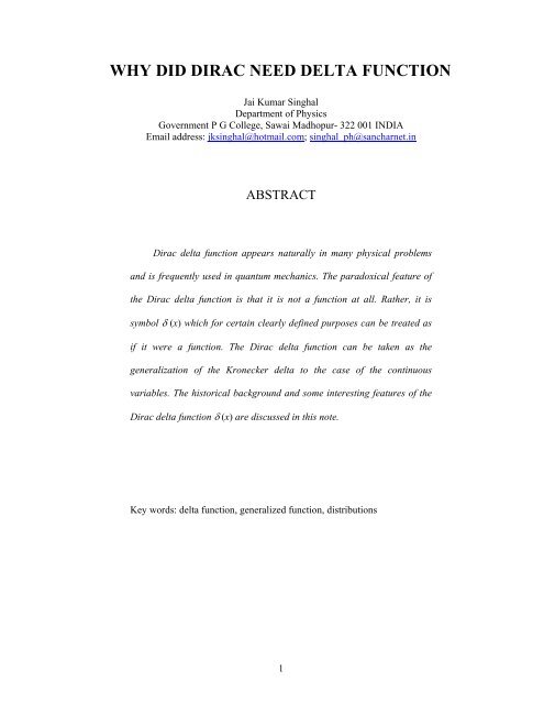
<strong>WHY</strong> <strong>DID</strong> <strong>DIRAC</strong> <strong>NEED</strong> <strong>DELTA</strong> <strong>FUNCTION</strong><br />
Jai Kumar Singhal<br />
<strong>Department</strong> <strong>of</strong> <strong>Physics</strong><br />
Government P G College, Sawai Madhopur- 322 001 INDIA<br />
Email address: jksinghal@hotmail.com; singhal_ph@sancharnet.in<br />
ABSTRACT<br />
Dirac delta function appears naturally in many physical problems<br />
and is frequently used in quantum mechanics. The paradoxical feature <strong>of</strong><br />
the Dirac delta function is that it is not a function at all. Rather, it is<br />
symbol δ (x) which for certain clearly defined purposes can be treated as<br />
if it were a function. The Dirac delta function can be taken as the<br />
generalization <strong>of</strong> the Kronecker delta to the case <strong>of</strong> the continuous<br />
variables. The historical background and some interesting features <strong>of</strong> the<br />
Dirac delta function δ (x) are discussed in this note.<br />
Key words: delta function, generalized function, distributions<br />
1
1. Introduction<br />
The delta functions appeared in the early days <strong>of</strong> 19 th century, in works <strong>of</strong> the<br />
Poission (1815), Fourier (1822) and Cauchy (1823). Subsequently O Heaviside (1883)<br />
and G Kirch<strong>of</strong>f (1891) gave the first mathematical definitions <strong>of</strong> the delta functions.<br />
P A M Dirac (1926) introduced delta function in his classic and fundamental work on<br />
the quantum mechanics. Dirac also listed the useful and important properties <strong>of</strong> the<br />
delta function. The uses <strong>of</strong> the delta function become more and more common<br />
thereafter. We call δ (x) as the Dirac delta function for historical reasons, while it is<br />
not a function <strong>of</strong> x in conventional sense, which requires a function to have a definite<br />
value at each point in its domain. Therefore δ (x) cannot be used in mathematical<br />
analysis like an ordinary function. In mathematical literature it is known as<br />
generalized function or distribution, rather than function defined in the usual sense. A<br />
definitive mathematical theory <strong>of</strong> distributions was given by L Schwartz (1950) in his<br />
Theorie des Distributions.<br />
The Dirac delta function is used to get a precise notation for dealing with<br />
quantities involving certain type <strong>of</strong> infinity. More specifically its origin is related to<br />
the fact that an eigenfunction belonging to an eigenvalue in the continuum is nonnormalizable,<br />
i.e., its norm is infinity.<br />
2. Why did Dirac need the delta function?<br />
Now we discuss why did Dirac need the delta function? Let us consider an<br />
arbitrary quantum mechanical state a . We can represent it by an expansion in a<br />
complete set <strong>of</strong> orthonormal basis states<br />
x i <strong>of</strong> a particular representation that is<br />
assumed to have n discrete basis states<br />
2
a = a1 x1<br />
+ a2<br />
x2<br />
+ ...............<br />
+ a n x n , (1)<br />
where the orthonormality condition is<br />
xi x j<br />
= δ<br />
(2)<br />
ij<br />
( δ ij is Kronecker delta; δ ij = 0 if i ≠ j and δ ij =1 if i = j).<br />
The (probability) amplitude <strong>of</strong> finding the state a in the base state<br />
x i is<br />
ϕ a<br />
(3)<br />
i =<br />
x i<br />
Due to orthonormality <strong>of</strong> the<br />
x i<br />
, Eq. (3) gives<br />
ϕ i = a i<br />
(4)<br />
i.e., the expansion coefficients (a i )defining a state a in a particular representation<br />
are simply amplitudes for finding the arbitrary state in the corresponding basis state.<br />
Eq. (1) can be written as<br />
a = ∑ x a<br />
(5)<br />
i<br />
i x i<br />
We want now to see how these relations must be modified when we are dealing<br />
with a continuum <strong>of</strong> base states. For this, consider the motion <strong>of</strong> a particle along a<br />
line. To describe the state ψ <strong>of</strong> the particle we can use the position representation.<br />
In this representation the basis states x describe a particle to be found at x and are<br />
continuous and non-denumerable. The most general state is<br />
ψ = a x + a x ............................., (6)<br />
1 1 2 2 +<br />
which is in analogy with Eq. (1). Since the states x are continuous we must replace<br />
sum in Eq. (5) by an integral, i.e.,<br />
ψ = ∫ f ( x)<br />
x dx , (7)<br />
where f (x) is the amplitude <strong>of</strong> finding the particle at position x. The amplitude <strong>of</strong><br />
finding the particle at position x’ is<br />
3
f ( x'<br />
) = x'<br />
ψ = ∫ f ( x)<br />
x'<br />
x dx . (8)<br />
This relation must be hold for any state ψ and therefore for any function f (x). This<br />
requirement should completely determine the amplitude f (x’), which is <strong>of</strong> course just<br />
a function that depends on x and x’.<br />
Now problem is to find a function<br />
x' x which when multiplied with f (x) and<br />
integrated over x gives the quantity f (x’). Suppose we take x’ = 0 and define the<br />
amplitude<br />
0 x to be some function <strong>of</strong> x (say g (x)) then Eq. (8) gives<br />
f<br />
( 0) = ∫ f ( x)<br />
g(<br />
x)<br />
dx . (9)<br />
What kind <strong>of</strong> function g (x) could possibly satisfy this? Since the integral must not<br />
depend on what values f (x) takes for values <strong>of</strong> x other than 0, g (x) must clearly be 0,<br />
for all values <strong>of</strong> x except 0. But if g (x) is 0 everywhere, the integral will be 0, too and<br />
Eq. (9) will not satisfied. So we are in a strange situation: we wish a function to be 0<br />
everywhere except at a point, and still to give a finite result. It turns out that there is<br />
no such mathematical function that will do this. Since we can not find such a function,<br />
the easiest way out is just to say the g (x) is defined by the Eq. (9), namely g (x) is that<br />
function, which makes Eq. (9) correct, and this relation must hold for any function<br />
(numerical, vector or linear operator). Dirac first did this and the function carries his<br />
name. It is written as δ (x).<br />
3. How δ (x−x 0 ) look like?<br />
The Dirac delta function is defined not by giving its values at different points but<br />
by giving a rule for integrating its product with a continuous function (Eq. (9)), if the<br />
origin is shifted form 0 to some point x 0 then Eq. (9) will be read as<br />
f ( x0 ) = ∫ δ ( x − x0<br />
) f ( x)<br />
dx . (10)<br />
4
Obviously, the contribution to the integral in Eq. (10) comes only from x = x 0 (i.e.,<br />
only the first term in the Taylor expansion <strong>of</strong> the function f (x) around the origin x 0. ),<br />
as for all other values <strong>of</strong> the function is zero. This relation must hold for any function.<br />
To have an understanding <strong>of</strong> δ (x−x 0 ), let us consider an arbitrary function that is<br />
non-zero everywhere except at point x 0 where it vanishes:<br />
f (x) = 0 at x = x 0<br />
= non-zero, everywhere else x = x 0 (11)<br />
In this case Eq. (10) gives<br />
∫ δ ( x − x0 ) f ( x)<br />
dx = 0<br />
(12)<br />
Since Eq. (12) must hold for any arbitrary form <strong>of</strong> the f (x) outside <strong>of</strong> the point x 0 , we<br />
conclude that δ (x−x 0 ) = 0, if x ≠ x 0 . Also from Eq. (10) δ (x−x 0 ) = ∞, if x = x 0 . Thus,<br />
we have δ (x−x 0 ) = 0 if x ≠ x 0<br />
= ∞ if x = x 0 (13)<br />
If we choose f (x) = 1, then defining relation (10) gives<br />
∫δ ( x − x0 ) dx = 1<br />
(14)<br />
i.e., the delta function is normalized to unity.<br />
All <strong>of</strong> these results show that the δ (x−x 0 ) can not thought <strong>of</strong> as a function in usual<br />
sense. However, it can be thought <strong>of</strong> as a limit <strong>of</strong> a sequence <strong>of</strong> regular functions.<br />
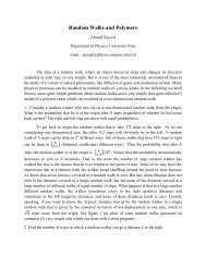
Schematically the delta function looks like a curve shown in Fig. 1, whose width<br />
tends to zero and the peak tends to infinity keeping the area under the curve finite.<br />
This curve represents a function <strong>of</strong> the real variable x, which vanishes everywhere<br />
except inside a small domain <strong>of</strong> length ε about the origin x 0 and which is so large<br />
inside this domain that its integral over the domain is unity; then in the limit ε → 0,<br />
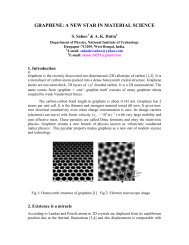
this function becomes δ (x−x 0 ). This curve may be visualized as a limit <strong>of</strong> more<br />
5
familiar curves, e.g., a rectangular curve <strong>of</strong> height 1/ε and width ε or isosceles<br />
triangles <strong>of</strong> height 2/ε and base ε. These are plotted in Fig. 2. The area under both the<br />
curves is 1 for all values <strong>of</strong> ε. In the limit ε → 0, the height becomes arbitrarily large<br />
and width shrinks to zero keeping area still 1. Thus these functions become Dirac<br />
delta function in the limit ε → 0.<br />
4. Representations<br />
As noted earlier, the delta function can be thought <strong>of</strong> a limit <strong>of</strong> a sequence <strong>of</strong><br />
regular functions. An infinite number <strong>of</strong> sequences may be constructed. Here we give<br />
some frequently used simple representations <strong>of</strong> the δ (x−x 0 ).<br />
(1) A representation <strong>of</strong> the δ (x) is given by<br />
⎛ sinLx<br />
⎞<br />
δ ( x)<br />
= Lim<br />
⎜<br />
⎟<br />
(15)<br />
L→<br />
∞ ⎝ π x ⎠<br />
This function for any L looks like a diffraction amplitude with width proportional to<br />
1/L. For any L the function is regular. As we increase the value <strong>of</strong> L the function<br />
peaks more strongly at x = 0, and hence in the limit L → ∞ it behaves like the delta<br />
function. Further, at x = 0,<br />
when x increases.<br />
⎛ sinLx<br />
⎟ ⎞<br />
⎜<br />
⎝ π x ⎠<br />
L 2π<br />
~ and its value oscillate with a period π L<br />
Also<br />
∞<br />
∫<br />
−∞<br />
⎛ sinLx<br />
⎞<br />
⎜<br />
⎟dx<br />
⎝ π x ⎠<br />
= 1<br />
(independent <strong>of</strong> the value <strong>of</strong> the x)<br />
and<br />
Thus the<br />
∞<br />
∫<br />
−∞<br />
⎛ sinLx<br />
⎞<br />
f ( x)<br />
⎜<br />
⎟ dx = f (0) .<br />
⎝ π x ⎠<br />
⎛ sinLx<br />
⎟ ⎞<br />
δ ( x)<br />
= Lim<br />
⎜ has all the properties <strong>of</strong> a δ (x).<br />
L→<br />
∞ ⎝ π x ⎠<br />
6
∞<br />
(2) Let us now consider the integral ∫<br />
e ikx<br />
−∞<br />
dk<br />
: This can be written as<br />
L<br />
Lim ∫ e dk =<br />
L→∞<br />
−L<br />
ikx<br />
Lim<br />
L→∞<br />
⎛ ikx<br />
⎜<br />
e − e<br />
−<br />
⎝ i x<br />
ikx<br />
⎞<br />
⎟<br />
⎠<br />
⎛ sinLx<br />
= ⎟ ⎞<br />
2 π Lim<br />
⎜ = 2π δ (x)<br />
L→∞<br />
⎝ π x ⎠<br />
⇒<br />
∞<br />
∫<br />
−∞<br />
1 ikx<br />
δ ( x)<br />
= e dk<br />
(16)<br />
2π<br />
The above relation is an alternate representation <strong>of</strong> δ (x). Here we immediately note<br />
that δ (x) is simply the Fourier transform <strong>of</strong> the constant<br />
1 .<br />
2π<br />
(3) Separating the real and imaginary parts in Eq. (16) we find<br />
∞<br />
∫<br />
−∞<br />
= 1<br />
δ ( x)<br />
cos kx<br />
2π<br />
dk<br />
(17)<br />
∞<br />
∫<br />
−∞<br />
= 1<br />
0 sin kx<br />
2π<br />
dk<br />
(18)<br />
Eq. (17) is one <strong>of</strong> the most commonly used explicit expressions for δ (x).<br />
(4) A useful representation <strong>of</strong> the δ (x) is<br />
δ ( x)<br />
α 2<br />
−α<br />
x<br />
= Lim e<br />
(19)<br />
α →∞ π<br />
This is the normalized Gaussian function <strong>of</strong> standard deviation<br />
1 , which tends to<br />
2α<br />
zero as α→ ∞. Its height is proportional to √α and it peaks at x = 0.<br />
Some useful representations that are encountered in various applications are<br />
(5) δ ( x ) =<br />
1 ⎛ α ⎞<br />
Lim ⎜ ⎟<br />
α →∞<br />
π 2 2<br />
⎝ x + α ⎠<br />
(20)<br />
(6) δ ( x)<br />
=<br />
d<br />
θ ( x)<br />
,<br />
dx<br />
(21)<br />
where θ (x) is the step function which is defined as a generalized function through<br />
7
θ (x) = 0 for x ≤ 0<br />
= 1 for x ≥ 0<br />
The three-dimensional Dirac delta function can be written by generalizing the onedimensional<br />
function i.e.,<br />
→ →<br />
− 0<br />
δ 3 ( r r ) = δ (x−x 0 ) δ (y−y 0 ) δ (z−z 0 ) (22)<br />
3<br />
→<br />
→<br />
3<br />
with ∫ δ ( r − r0<br />
) d r = ∫∫∫ δ ( x − x0<br />
) δ ( y − y0<br />
) δ ( z − z0<br />
) dxdydz = 1<br />
3<br />
→<br />
→<br />
and ∫ δ ( r − r0<br />
) f ( r ) d r = f ( r0<br />
)<br />
5. Delta function in physical problems<br />
→<br />
3<br />
→<br />
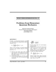
The Dirac delta function arises naturally in many branches <strong>of</strong> science and<br />
engineering. To appreciate this, let us consider the divergence <strong>of</strong> function<br />
→<br />
A =<br />
rˆ<br />
r<br />
2<br />
(a<br />
basic problem <strong>of</strong> electrodynamics)[1]. As shown in Fig. 3 → A is spreading radially<br />
outward and has a large positive divergence, but we get zero by actual calculation as<br />
shown below (in radial coordinates):<br />
→<br />
1 ∂ ⎛ 2 1 ⎞ 1 ∂<br />
∇ .<br />
→ A = ⎜r<br />
⎟ = () 1 = 0<br />
2 ∂ 2 2<br />
r r ⎝ r ⎠ r ∂r<br />
(21)<br />
The surface integral <strong>of</strong> → A over a sphere <strong>of</strong> radius R centered at origin (r = 0) is<br />
→ →<br />
π 2π<br />
1 2<br />
∫ A . ds = ∫ ( R sinθ<br />
dθ<br />
dφ)<br />
= ∫sinθ<br />
dθ<br />
∫dφ<br />
= 4π<br />
(22)<br />
2<br />
R<br />
On the other hand from divergence theorem, we have<br />
→ →<br />
→<br />
→<br />
0<br />
∫ ∇. A dv = ∫ A.<br />
ds = 4π<br />
(23)<br />
0<br />
8
Thus we are in a paradoxical situation, in which ∇ → . →<br />
A = 0 but its integral is 4π. The<br />
source <strong>of</strong> this inconsistency lies at the origin, where the → A blows up, although<br />
∇ → . →<br />
A = 0 everywhere except at the origin. From Eq. (23) it is evident that<br />
∫<br />
∇ → →<br />
→<br />
. A dv = 4π for any sphere centered at origin irrespective <strong>of</strong> its size. Hence<br />
→<br />
∇ . A has a strange property that it vanishes everywhere except at the origin, and yet<br />
its integral is 4π. We also have the similar problem <strong>of</strong> a point particle: density (charge<br />
density) is zero everywhere except at its location, yet it’s integral i.e., mass (charge) is<br />
finite. No mathematical functions behave like this but we note that these are precisely<br />
the defining properties <strong>of</strong> the Dirac delta function (see Eqs 13 and 14). Hence these<br />
contradictions can be avoided by introducing the Dirac delta function; one can write<br />
→<br />
rˆ<br />
∇ .<br />
2<br />
r<br />
3<br />
→<br />
= 4π<br />
δ ( r )<br />
6. Properties <strong>of</strong> the Dirac delta function<br />
We list below some properties <strong>of</strong> the Dirac delta function without assuming any<br />
particular representation. In fact, these properties are equations, which are essentially<br />
rules for manipulations for algebraic work involving δ (x) functions. The meaning <strong>of</strong><br />
these equations is that the left and right hand sides when used as a multiplying factor<br />
under an integrand leads to the same results.<br />
(i)<br />
δ (x) = δ (−x)<br />
(ii)<br />
δ* (x) = δ (x)<br />
(iii) x δ (x) = 0<br />
9
(iv) δ (ax) =<br />
1 δ (x) (a > 0)<br />
a<br />
(v)<br />
f (x) δ (x−a) = f (a) δ (x−a)<br />
(vi) ∫ dxδ ( x)<br />
f ( x)<br />
= f (0)<br />
(vii) ∫ dxδ<br />
( a − x)<br />
δ ( x − b)<br />
= δ ( a − b)<br />
(viii) δ’ (−x) = −δ’ (x) where δ’ (x) =<br />
d δ (x)<br />
dx<br />
(ix) ∫ dxδ '(<br />
x)<br />
f ( x)<br />
= − f '(0)<br />
(x)<br />
2 2 δ ( x − a)<br />
+ δ ( x + a)<br />
δ ( x − a ) =<br />
(a > 0)<br />
2a<br />
Further suggested reading:<br />
1) D J Griffiths, Introduction to Electrodynamics, Prentice Hall <strong>of</strong> India Private<br />
Limited, 1997 p. 46.<br />
2) R P Feynman, R B Leighton and M Sands, The Feynman Lectures on <strong>Physics</strong> Vol.<br />
III Quantum Mechanics, Narosa Publishing Housing, New Delhi, 1986 (See<br />
chapter 16).<br />
3) P A M Dirac, The Principles <strong>of</strong> Quantum Mechanics, Oxford University Press, IV<br />
Edition 1985, p 58.<br />
4) Ashok Das and A C Melissinos, Quantum Mechanics A Modern Introduction,<br />
Gorden and Breach Science Publishers, 1986.<br />
10