8. The Heckscher-Ohlin model - WIF
8. The Heckscher-Ohlin model - WIF
8. The Heckscher-Ohlin model - WIF

You also want an ePaper? Increase the reach of your titles
YUMPU automatically turns print PDFs into web optimized ePapers that Google loves.
<strong>8.</strong> <strong>The</strong> <strong>Heckscher</strong>-<strong>Ohlin</strong> <strong>model</strong><br />
<strong>8.</strong>1. Introduction<br />
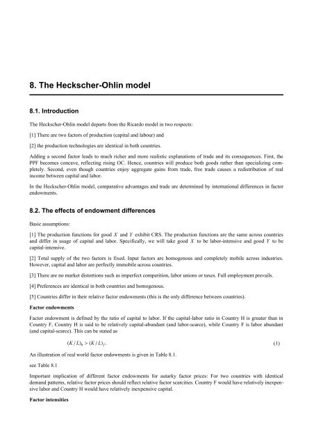
<strong>The</strong> <strong>Heckscher</strong>-<strong>Ohlin</strong> <strong>model</strong> departs from the Ricardo <strong>model</strong> in two respects:<br />
[1] <strong>The</strong>re are two factors of production (capital and labour) and<br />
[2] the production technologies are identical in both countries.<br />
Adding a second factor leads to much richer and more realistic explanations of trade and its consequences. First, the<br />
PPF becomes concave, reflecting rising OC. Hence, countries will produce both goods rather than specializing completely.<br />
Second, even though countries enjoy aggregate gains from trade, free trade causes a redistribution of real<br />
income between capital and labor.<br />
In the <strong>Heckscher</strong>-<strong>Ohlin</strong> <strong>model</strong>, comparative advantages and trade are determined by international differences in factor<br />
endowments.<br />
<strong>8.</strong>2. <strong>The</strong> effects of endowment differences<br />
Basic assumptions:<br />
[1] <strong>The</strong> production functions for good X and Y exhibit CRS. <strong>The</strong> production functions are the same across countries<br />
and differ in usage of capital and labor. Specifically, we will take good X to be labor-intensive and good Y to be<br />
capital-intensive.<br />
[2] Total supply of the two factors is fixed. Input factors are homogenous and completely mobile across industries.<br />
However, capital and labor are perfectly immobile across countries.<br />
[3] <strong>The</strong>re are no market distortions such as imperfect competition, labor unions or taxes. Full employment prevails.<br />
[4] Preferences are identical in both countries and homogenous.<br />
[5] Countries differ in their relative factor endowments (this is the only difference between countries).<br />
Factor endowments<br />
Factor endowment is defined by the ratio of capital to labor. If the capital-labor ratio in Country H is greater than in<br />
Country F, Country H is said to be relatively capital-abundant (and labor-scarce), while Country F is labor abundant<br />
(and capital-scarce). This can be stated as<br />
HK ê LL h > HK ê LL f .<br />
(1)<br />
An illustration of real world factor endowments is given in Table <strong>8.</strong>1.<br />
see Table <strong>8.</strong>1<br />
Important implication of different factor endowments for autarky factor prices: For two countries with identical<br />
demand patterns, relative factor prices should reflect relative factor scarcities. Country F would have relatively inexpensive<br />
labor and Country H would have relatively inexpensive capital.<br />
Factor intensities
2 Class_7.nb<br />
Good Y is relatively capital-intensive and good X is relatively labor-intensive if the capital-labor ratio used in production<br />
is higher in the Y -sector<br />
HK ê LL y > HK ê LL x .<br />
(2)<br />
In equilibrium, both sectors choose capital-labor ratios that minimize costs taking the prevailing relative factor price<br />
w=w ê r into account (the choosen capital-labor ratio is endogenous). In principle, the factor intensities could be<br />
reversed when factor prices change. We assume here that this is not the case (no factor intenstity reversal).<br />
Table <strong>8.</strong>2 presents estimates of capital-labor ratios in certain U.S. manufacturing industries in 1984.<br />
see Table <strong>8.</strong>2<br />
Implications<br />
Consider the endowment represented by point E in Figure <strong>8.</strong>1 (L êê and K êê ). <strong>The</strong> associated maximum quantities of X<br />
and Y are X êêê and Y êê as shown in Figure <strong>8.</strong>2. <strong>The</strong> complete PPF is Y<br />
êê X<br />
êêê . (E will be E f in the argumentation below)<br />
Now consider the endowment E h . Once more, the maximum level of output (isoquants in Figure <strong>8.</strong>1) is indicated by<br />
Y êê<br />
h and X êêê h in Figure <strong>8.</strong>2. <strong>The</strong> corresponding PPF is Y êê h X êêê h . Compared to F, more Y (capital-intensive good) and less<br />
X (labor-intensive good) can be produced.<br />
see Figure <strong>8.</strong>1<br />
see Figure <strong>8.</strong>2<br />
Scale invariance: Notice that the scale of the economies does not influence the basic argument according to which<br />
relative factor endowment is crucial for comparative advantages. This is due to the fact that the production functions<br />
are assumed homogenous.<br />
Figure <strong>8.</strong>3 reproduces the PPFs of the two countries together with a set of (identical) indifferences curves, reflecting<br />
identical and homogenous preferences.<br />
see Figure <strong>8.</strong>3<br />
In addition, the autarky equilibrium points are shown. Notice that in autarky we have<br />
p h > p f .<br />
(3)<br />
Recall that p := p x ê p y , i.e. X is relatively expensive at H and relatively cheap at F (vice versa for Y ).<br />
Because of homogeneity of production functions and preferences, these relative autarky prices would be the same<br />
regardless of country size (equilibrium points would lie along rays 0A h and 0A f generating the same prices). Absolute<br />
size is irrelevant for the determination of comparative advantage in the HO <strong>model</strong>. What matters are relative factor<br />
endowments and factor intensities.<br />
<strong>8.</strong>3. <strong>The</strong> <strong>Heckscher</strong>-<strong>Ohlin</strong> theorem<br />
What are the consequences of opening up the economies in an HO world?<br />
In autarky, p h > p f . With international trade, the residents of H have incentives to purchase X abroad (in F) and,<br />
analoguosly, the residents of F will purchase Y in country H. This applies as long as p h > p f .<br />
This demand shift induces a change in commodity prices and thereby a change in national production structures. <strong>The</strong><br />
production point in H (F) will shift toward the Y (X ) axis. As a result, p h decreases and p f increases. In an international<br />
equilibrium, commodotity prices are equalized in the two countries p * = p h = p f .<br />
An international equilibrium additionally requires that world commodity markets clear. For each good, excess demand<br />
from one country must equal excess supply from the other country. In Figure <strong>8.</strong>4, the trade triangles must be of<br />
identical size.
Class_7.nb 3<br />
see Figure <strong>8.</strong>4<br />
Both economies consume on indifference curves that lie outside their PPF. <strong>The</strong>refore, free trade in the HO <strong>model</strong><br />
provides aggregate gains from trade for each country.<br />
<strong>Heckscher</strong>-<strong>Ohlin</strong> theorem<br />
Given the assumptions of the <strong>model</strong> (stated above), a country will export the commodity that intensively uses its<br />
relatively abandunt factor.<br />
By virtue of exporting the capital-intensive good and importing the the labor-intensive good, Country H implicitly<br />
exports the services of capital. International trade in commodities accomplishes the task of exchanging surplus factor<br />
services between countries.