"Monte Carlo Estimates of the Log Determinant of ... - Spatial Statistics

R.P. Barry, R.K. Pace / Linear Algebra and its Applications 289 (1999) 41±54 49
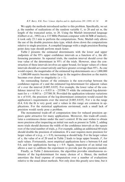
We apply the methods introduced earlier to this problem. Speci®cally, we set
p, the number of realizations of the random variable V i , to 20 and set m, the
length of the truncated series, to 20. Using the Matlab interpreted language
(Gilbert et al., 1992) on a 133 MHz Pentium computer with 64 MB of memory,
it took only 23.1 min to perform the computations. Note, Matlab only allows
the use of the double precision data type, which slows down the computations
relative to single precision. A compiled language with a single precision ¯oating
point data type should perform much faster.
Table 2 presents the estimated determinants with the lower and upper
endpoints of the 95% upper con®dence intervals as a function of a, the differencing
parameter. In repeated trials, the random interval should cover the
true value of the determinant in 95% of the trials. However, since the construction
of these intervals involves an upper bound, for larger values of a these
intervals should act conservatively and have greater coverage than 95%. As one
would expect, the magnitudes of the estimated log-determinants on a 1,000,000
1,000,000 matrix become rather large in the negative direction as the matrix
becomes ever closer to singularity …a ˆ 1†.
An outstanding feature of the estimates is the non-overlap between the
con®dence regions of a and the estimated log-determinant for adjacent values
of a over the interval ‰0:005; 0:835Š. For example, the lower value of the con-
®dence interval for a ˆ 0:835 is 235506:75 while the estimated log-determinant
for a ˆ 0:845 is 237380:58. Provided the application tolerates variations
in a of 0:01, the precision of the log-determinant estimation would exceed the
application's requirements over the interval ‰0:005; 0:835Š. For a in the range
(0.4, 0.6) the ®t is very good, and a values in this range are common in applications.
For the statistical applications envisioned, such a small lack of
precision would rarely pose a problem.
The monumental trade-o€ of computation time for reduced precision appears
quite attractive for many applications. Moreover, this trade-o€ constitutes
a continuous choice under the user's control. If the user wishes to obtain
more precision after inspecting an initial run such as present in Table 2, adding
more trials should decrease the width of the con®dence intervals at the square
root of the total number of trials, p. For example, adding an additional 60 trials
should double the precision of estimation. If a user requires more precision for
larger values of a (e.g., a > 0:9), increasing m should help. For the larger values
of a, the value of m of 20 used in Table 2 leads to large upper bounds, F , for
such values. Fortunately, most empirical applications have a between 0.4 and
0.6, and few applications having a > 0:9. Again, inspection of an initial run
allows a user to calibrate the experiment to provide just the precision needed.
Finally, as Table 2 demonstrates, the algorithm provides simultaneous estimates
of the log-determinant for many choices of a. Hence, the method
amortizes the ®xed expense of computation over a number of evaluations
relative to the usual direct methods. Not only does this greatly save time, but it