1 Differential Forms - Caltech
1 Differential Forms - Caltech
1 Differential Forms - Caltech

You also want an ePaper? Increase the reach of your titles
YUMPU automatically turns print PDFs into web optimized ePapers that Google loves.
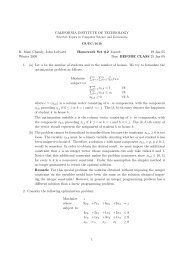
ˆω k<br />
ˆd k<br />
−−−−−→ ˆω k+1<br />
φ k ⏐↓<br />
⏐↓φ k+1<br />
ω k d k<br />
−−−−−→ ω k+1<br />
where ˆω k is a discrete k-form and ω k is a smooth k-form. Consider a simplicial 2-complex K and prove that<br />
this relationship holds in the case of k = 0, i.e., show that<br />
for any discrete 0-form ω on K.<br />
φ 1 ˆd 0 ˆω = d 0 φ 0 ˆω<br />
(Hint: consider a single 2-simplex; the results of the previous three exercises will be useful.)<br />
Coding 2. Write a MATLAB routine that interpolates a discrete 1-form over a single 2-simplex in the plane<br />
using the Whitney 1-form bases, starting with the template below. (In other words, implement the expression<br />
derived in Exercise 3.) This routine will be used to display the vector field decomposition produced in a later<br />
exercise. You may find it useful to use the subroutine A = triangle area( a, b, c ). Additionally, you<br />
should test your routine by running the script draw whitney oneform.m. This script produces an output file<br />
oneform.ps which displays the Whitney 1-form basis for a single edge in a triangle and should match the<br />
appearance of the illustration above. Please include a printout of this output with your written assignment.<br />
function u = oneform( V, omega, p )<br />
% function u = oneform( V, omega, p )<br />
%<br />
% Interpolates a discrete 1-form using the Whitney basis.<br />
%<br />
% INPUT:<br />
% V - 2x3 matrix; columns give vertex coordinates of vertices in triangle {a,b,c}<br />
% omega - 3x1 vector of 1-form values stored on edges (a,b), (b,c), (c,a), resp.<br />
% p - 2x1 vector representing sample location<br />
%<br />
% OUTPUT:<br />
% u - 2x1 vector giving interpolated 1-form at p<br />
%<br />
2.3 Discrete Exterior Derivative<br />
Recall that the smooth exterior derivative d maps a k-form to a (k + 1)-form. In our discrete framework, this<br />
means we want an operator that maps a scalar quantity stored on k-dimensional simplices to a scalar quantity<br />
on (k + 1)-dimensional simplices. The discrete version of the exterior derivative turns out to be a very simple<br />
procedure: to get the scalar value for a particular (k + 1)-simplex, we basically just add up the values stored on<br />
all the k-simplices along its boundary! With one caveat: we need to be careful about orientation. Since the sign<br />
of the scalar value changes depending on the orientation of each simplex (and since this choice is arbitrary),<br />
we need to take orientation into account in our sum. In general this means that if the orientation of a simplex<br />
and one of the simplices on its boundary are opposite, we subtract the value stored on the boundary simplex<br />
from our sum; otherwise, we add this value.<br />
For instance, in the special case of a 0-form (i.e., a scalar function on vertices), the exterior derivative is<br />
incredibly simple to compute: to get the scalar value for an edge whose orientation is from a to b, simply<br />
subtract the value at a from the value at b!<br />
Exercise 6. Let α be the discrete 1-form on the mesh pictured below given by the following table:<br />
e 1 2<br />
e 2 -1<br />
e 3 3<br />
e 4 -4<br />
e 5 7<br />
6