1 Differential Forms - Caltech

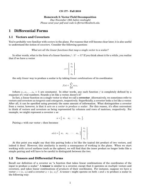
CS 177 - Fall 2010
Homework 3: Vector Field Decomposition
Due November 18th before midnight
Please send your pdf and code to fferrari@caltech.edu
1 Differential Forms
1.1 Vectors and Covectors
You’re probably very familiar with vectors in the plane. For reasons that will become clear later, it is also useful
to understand the notion of covectors. Consider the following question:
What are all the linear functions that map a single vector to a scalar?
In other words, what is the form of a linear function f : R n → R? If you think about it for a while, you realize
that if we have a vector
⎡
x =
⎢⎣
the only linear way to produce a scalar is by taking linear combinations of its coordinates:
n∑
f (x) = α i x i ,
x 1
x 2
.
x n
i=1
(where α 1 , α 2 , . . . , α n ∈ R are constants). In other words, any such function f is completely defined by a
sequence of n real numbers. Sounds a lot like a vector, doesn’t it?
In fact, a linear function on a single vector is what we call a covector. Alternatively, we sometimes refer to
vectors and covectors as tangents and cotangents, respectively. Superficially, a covector looks a lot like a vector.
After all, it can be specified using precisely the same amount of information. What distinguishes a covector
from a vector, however, is that it acts on a vector to produce a scalar. For this reason, it’s often convenient
to think of vectors and covectors as being represented by columns and rows of matrices, respectively. For
example, we might represent a covector α as
Pairing α with our vector x then becomes
,
⎤⎥⎦
α = [ α 1 α 2 · · · α n
]
.
α(x) = [ α 1 α 2 · · · α n
]
At this point you might say that this pairing looks a lot like the typical dot product of two vectors, and
indeed it does! However, this similarity is merely a consequence of working in the plane. When we start
working with curved surfaces (such as the sphere), we will find that the inner product no longer looks like a
simple pairing and will have to be careful to distinguish between the two.
1.2 Tensors and Differential Forms
Recall our definition of a covector as “a function that takes linear combinations of the coordinates of the
input to produce a scalar.” A tensor is similar to a covector, except that it operates on multiple vectors and
covectors, and takes linear combinations of products of their coordinates. For instance, suppose we have a
vector x = [x 1 x 2 ] and a covector α = [α 1 α 2 ] T . A tensor t might operate on both x and α to produce a scalar in
the following way:
⎡
⎢⎣
x 1
x 2
.
x n
.
⎤⎥⎦
1

t(x, α) = 3x 1 α 1 − x 1 α 2 + 4x 2 α 2 .
In this case, we can also express t using matrix notation:
t(x, α) = [ α 1 α 2
] [ 3 0
−1 4
] [ ]
x1
.
x 2
In general, however, a tensor may map many vectors and covectors to a scalar – not just one of each – so we
cannot always express it as a matrix operation. If a tensor maps k vectors and l covectors to a scalar, we call it
a “k-times covariant, l-times contravariant” tensor.
Finally, a differential form or differential k-form is a k-times covariant antisymmetric tensor. In other
words, it’s an object that eats k vectors and spits out a scalar (in a linear way!), and whose sign changes if we
swap any pair of arguments. For instance, if α is a 3-form and u, v, and w are vectors, then
α(u, v, w) = −α(w, v, u),
etc. Note that a differential 1-form is the same thing as a covector! Differential forms play an important
role in geometry and physics, and are often used to represent physical quantities as we’ll see in some of our
applications. Finally, it is important to note that while most authors make a linguistic distinction between a
“vector” and a “vector field,” many do not make the distinction between a “differential form” and a “differential
form field” – the former is simply used interchangeably.
2 Exterior Calculus
You’re probably familiar with vector calculus which consists of operations on “primal” objects such as vector
fields. It is also possible to define an exterior calculus that consists of operations on “dual” objects such
as covectors and differential forms. The duality between the two makes it possible to define any differential
operator from vector calculus using the language of exterior calculus. One reason why this approach is nice
from a practical point of view is that exterior calculus has only a single differential operator, called the exterior
derivative, which is denoted d. In the discrete setting, this means that only one differential operator ever has
to be defined and implemented. Here are a few typical differential operators from vector calculus expressed
using the exterior derivative 1 ∇ f = d f
∇ × F = ⋆dF
∇ · F = ⋆d ⋆ F
The additional map ⋆ is called the Hodge star and introduces another kind of duality within exterior calculus
– we will discuss the Hodge star in more detail later. It is also important to note that covector fields are a
special case of something called a differential form. In particular, covector fields are referred to as 1-forms and
“look” much like vector fields. Another common special case is the 0-form, which can be thought of as a scalar
field. You will often see differential forms written in coordinate notation where the magnitude is given for each
principal direction. For example, a 1-form α = dx − ydz basically looks like a vector field whose magnitude is
1 in the x-direction, 0 in the y-direction, and −y in the z-direction. Much like the gradient operator maps a
scalar field to a vector field, the exterior derivative will map a 0-form to a 1-form. More generally, the exterior
derivative maps a k-form to a (k + 1)-form. Finally, the exterior derivative has the important property that
d ◦ d = 0.
2.1 Discrete Exterior Calculus
In order to actually compute with exterior calculus, we need to define a discrete exterior calculus (DEC) that
operates on quantities defined over some discrete differential geometry. In particular, we will define discrete
differential forms as quantities stored on simplicial meshes 2 , and discrete differential operators that act on
these forms in a way that faithfully mirrors the behavior of the smooth operators.
1 Technically speaking these operators are not identical since the operators from vector calculus operate on the tangent bundle whereas
the operators from exterior calculus operate on the cotangent bundle. Since these two spaces are dual, however, there exists a pair of very
simple operators ♯ (sharp) and ♭ (flat) which can be used to convert an object from vector calculus to exterior calculus and then back again.
For instance, we should really write ∇ × F = [ ⋆ ( dF ♭)] ♯ if we want the two operations to be truly identical maps.
2 Most operations in DEC are well-defined for more general cell complexes, but we will stick to simplicial complexes for simplicity.
2

2.2 Discrete Differential Forms
Discrete differential forms actually have a very simple representation: a k-form is represented by a single
scalar quantity at each k-dimensional simplex of the mesh. So for instance, a 0-form stores a scalar value at
each vertex, a 1-form stores a scalar value at each edge, etc. For 0-forms, you should think of this scalar as
simply a point sample of a scalar-valued function. For 1-forms, you should think of this scalar as the total
circulation along that edge. In other words, if you think of a smooth covector field as passing over an edge,
then the scalar will tell you how much total “stuff” is moving parallel to that edge. In general, you can think
of a discrete k-form as the integral of the evaluation of a smooth k-form over each k-simplex.
In addition to knowing how much stuff is moving through each simplex, we also need to know in which
direction the stuff is moving. In other words, if we have an edge between vertices a and b, we need to know
whether the stuff is flowing from a to b or from b to a. Hence, we give each edge an orientation (either a to
b or b to a) that gives us a canonical direction along which stuff flows. Then a positive scalar on this edge
indicates that stuff is flowing in the canonical direction, and a negative scalar indicates that stuff is flowing in
the opposite direction. It doesn’t matter how we pick this orientation as long as we are consistent.
2.2.1 Discretizing Smooth Forms
Quite often, integration of a smooth form over a simplex is done via numerical quadrature. Numerical quadrature
picks a collection of quadrature points x i and corresponding quadrature weights w i , and approximates an
integral using a weighted sum of function values at the quadrature points. For example, the integral of a
function f over a domain Ω would be approximated as
∫
∑
f (x)dx ≈ V(Ω) w i f (x i )
Ω
where V(Ω) is the volume of Ω.
For functions defined over simplices, there are a number of possible choices for weights and quadrature
points – the choice of which quadrature to use depends on the desired accuracy and the degree of the function
being integrated. For instance, one-point Gaussian quadrature on a simplex places a single quadrature point
of weight one at the barycenter of the simplex; for a linear function f , this choice of quadrature will in fact give
the exact answer.
Exercise 1. Given the oriented simplicial complex depicted below and the smooth 1-form ω = 2xdy − ydx,
compute the corresponding discrete 1-form (i.e., give the value stored on each edge).
i
(0,1)
(1,1)
e 1
e 2
e 3
e 5
e 4
(0,0) (1,0)
Coding 1. Starting with the template below, write a MATLAB routine that discretizes the smooth 1-form
ω(x, y) = 2e −(x2 +y 2) ((x + y)dx + (y − x)dy) .
Approximate the integral over each edge with a single quadrature point located at the edge midpoint.
You can test whether your routine is working properly by temporarily replacing ω with the linear 1-form
ω = 2xdy − ydx and running it on the mesh file test.obj, which corresponds to the discretization perfomed in
the previous exercise.
3

function omega = discretize_oneform( V, E )
% function omega = discretize_oneform( V, E )
%
% INPUT:
% V - dense 2x|V| matrix of vertex positions
% E - dense |E|x2 matrix of edges as 1-based indices into vertex list
%
% OUTPUT:
% omega - |E|x1 vector of discrete 1-form values stored on edges
%
2.2.2 Interpolating Discrete Forms
1
v
0
0
Although we can generally perform all of our computations directly using discrete differential forms, it is
sometimes necessary to construct a smooth form corresponding to a discrete form. One way to construct such
a form is via interpolation. The Whitney forms or Whitney bases provide a set of smooth forms that interpolate
discrete forms defined on a simplicial complex.
The Whitney 0-forms are basis elements for forms defined on vertices, and are denoted φ i where i is the
vertex of interest. In fact, φ i is simply the hat function on vertex i, i.e., the unique function that equals one at
vertex i, zero at all other vertices, and is affine over each 2-simplex (see illustration above, left).
Whitney 1-forms interpolate values stored on edges, and are denoted φ i j where the edge of interest is oriented
away from vertex i and toward vertex j. The 1-form bases can be expressed in terms of the 0-form
bases:
φ i j = φ i dφ j − φ j dφ i
where d is the (smooth) exterior derivative on 0-forms – see the next section for details. Notice that the
orientation of the edge (i to j vs. j to i) does matter here since φ i j is antisymmetric with respect to i and j,
i.e., φ i j = −φ ji . An illustration of a discrete 1-form on a triangle interpolated using the Whitney 1-form basis is
shown above (right). Edge labels indicate the value of the discrete form on each edge and arrows indicate the
direction and magnitude of the interpolated field.
The Whitney 2-forms interpolate values stored on faces, and are denoted φ i jk where the face of interest
contains vertices i, j, and k. The 2-form bases are simply piecewise constant functions that equal 1/A inside
the face (i, j, k) and zero elsewhere, where A is the area of the face.
(Note: you may wish to read the section on the exterior derivative before continuing with the following
exercises.)
4

Exercise 2. The barycentric coordinates for a point p in a simplex σ give, roughly speaking, the proximity of
p to each of the vertices of σ. More specifically, the ith barycentric coordinate function λ i : |σ| → R is the unique
affine function that equals one at vertex i and zero at all other vertices. In other words, λ i (v j ) = δ i j (where δ is
the Kronecker delta). Make a (simple!) argument that on a 2-simplex, λ i (p) is the same as the ratio
f (p) =
〈p, j, k〉
〈i, j, k〉
where j and k are the indices of the other two vertices in the 2-simplex and 〈i, j, k〉 denotes the area of the
triangle with vertices v i , v j , and v k .
v i
p
v j
v k
(Hint: think about the gradient of the area of a triangle. In the remaining exercises, you may find it convenient
to denote the rotation in the plane of a vector v by an angle π/2 by v ⊥ .)
Exercise 3. Derive an expression for Whitney 1-form bases on a simplicial 2-complex that is suitable for
implementation. In particular, for a 2-simplex σ with vertices v i , v j , and v k , give an expression for φ i j (p) purely
in terms of triangle areas and edge vectors, where p is any point inside the simplex.
(Hint: the Whitney 0-form bases restricted to a single simplex are merely the barycentric coordinate functions
for that simplex.)
Exercise 4.
Let e 1 , e 2 , and e 3 be the three edge vectors of a triangle oriented as in the figure below. Show that
(This fact will be useful in the next exercise.)
e ⊥ 2 + e⊥ 3 = −e⊥ 1 .
e 1
e 2
e 3
e 1
e 2
e 3
Exercise 5. One nice property of Whitney forms is that interpolating with Whitney forms and then applying
the (smooth) exterior derivative is the same as applying the (discrete) exterior derivative and then interpolating
with Whitney forms. In other words, the following diagram commutes:
5

ˆω k
ˆd k
−−−−−→ ˆω k+1
φ k ⏐↓
⏐↓φ k+1
ω k d k
−−−−−→ ω k+1
where ˆω k is a discrete k-form and ω k is a smooth k-form. Consider a simplicial 2-complex K and prove that
this relationship holds in the case of k = 0, i.e., show that
for any discrete 0-form ω on K.
φ 1 ˆd 0 ˆω = d 0 φ 0 ˆω
(Hint: consider a single 2-simplex; the results of the previous three exercises will be useful.)
Coding 2. Write a MATLAB routine that interpolates a discrete 1-form over a single 2-simplex in the plane
using the Whitney 1-form bases, starting with the template below. (In other words, implement the expression
derived in Exercise 3.) This routine will be used to display the vector field decomposition produced in a later
exercise. You may find it useful to use the subroutine A = triangle area( a, b, c ). Additionally, you
should test your routine by running the script draw whitney oneform.m. This script produces an output file
oneform.ps which displays the Whitney 1-form basis for a single edge in a triangle and should match the
appearance of the illustration above. Please include a printout of this output with your written assignment.
function u = oneform( V, omega, p )
% function u = oneform( V, omega, p )
%
% Interpolates a discrete 1-form using the Whitney basis.
%
% INPUT:
% V - 2x3 matrix; columns give vertex coordinates of vertices in triangle {a,b,c}
% omega - 3x1 vector of 1-form values stored on edges (a,b), (b,c), (c,a), resp.
% p - 2x1 vector representing sample location
%
% OUTPUT:
% u - 2x1 vector giving interpolated 1-form at p
%
2.3 Discrete Exterior Derivative
Recall that the smooth exterior derivative d maps a k-form to a (k + 1)-form. In our discrete framework, this
means we want an operator that maps a scalar quantity stored on k-dimensional simplices to a scalar quantity
on (k + 1)-dimensional simplices. The discrete version of the exterior derivative turns out to be a very simple
procedure: to get the scalar value for a particular (k + 1)-simplex, we basically just add up the values stored on
all the k-simplices along its boundary! With one caveat: we need to be careful about orientation. Since the sign
of the scalar value changes depending on the orientation of each simplex (and since this choice is arbitrary),
we need to take orientation into account in our sum. In general this means that if the orientation of a simplex
and one of the simplices on its boundary are opposite, we subtract the value stored on the boundary simplex
from our sum; otherwise, we add this value.
For instance, in the special case of a 0-form (i.e., a scalar function on vertices), the exterior derivative is
incredibly simple to compute: to get the scalar value for an edge whose orientation is from a to b, simply
subtract the value at a from the value at b!
Exercise 6. Let α be the discrete 1-form on the mesh pictured below given by the following table:
e 1 2
e 2 -1
e 3 3
e 4 -4
e 5 7
6

Compute the discrete 2-form dα, paying careful attention to orientation.
Exercise 7. The discrete exterior derivative on k-forms can be represented by a matrix d k ∈ R m×n where n is
the number of k-simplices in the complex, m is the number of (k + 1)-simplices. Entry (i, j) of d k equals ±1 if the
ith (k + 1)-simplex contains the jth k-simplex, where the sign is positive if the orientations of the two simplices
agree and negative otherwise. (All other entries in the matrix are zero.) Compute the matrix representations
for d 0 and d 1 on the mesh pictured below, and verify that d 1 d 0 = 0.
v 4
v 3
f 1
f 2
e 1
e 2
e 3
e 4
v 1
e 5
v 2
Coding 3. Write a MATLAB routine that builds (sparse!) matrices representing the discrete exterior derivatives
on 0- and 1-forms, starting with the template below. Edges should be oriented such that each edge points
from the smaller to the larger index. Faces should be oriented according to the input. The input to this routine
is slightly different than in the previous assignment: rather than a pair (V, F) where each row of F is a list
of vertex indices for a face, the routine accepts a triple (V, E, F) where each row of E gives a pair of vertex
indices defining an edge and each row of F gives a triple of edge indices defining a face. Additionally, the sign
of edge indices indicates whether they agree (positive) or disagree (negative) with the orientation of that face.
The routine [V,E,F] = read mesh( filename ) (provided) produces data in this format from a Wavefront
OBJ mesh. You can test your code by running it on the mesh test.obj – this mesh corresponds to the one
used in the previous exercise 3 You should also test that repeated application of the exterior derivative equals
zero, i.e., that d1*d0 yields a matrix of all zeros in MATLAB.
function [d0,d1] = build_exterior_derivatives( V, E, F )
% function [d0,d1] = build_exterior_derivatives( V, E, F )
%
% INPUT:
% V - dense 2x|V| matrix of vertex positions
% E - dense |E|x2 matrix of edges as 1-based indices into vertex list
% F - dense |F|x3 matrix of faces as 1-based indices into edge list
%
% OUTPUT:
% d0 - sparse |E|x|V| matrix representing discrete exterior derivative on 0-simplices
% d1 - sparse |F|x|E| matrix representing discrete exterior derivative on 1-simplices
%
2.3.1 Mesh Traversal
Because the matrices d 0 and d 1 contain indicence information, they can also be used to traverse the mesh. In
MATLAB, these matrices can be used in conjunction with the commands find and unique to iterate over
mesh elements in a number of ways. For instance, suppose we wish to visit each face in the mesh and grab the
indices of its three vertices. We might write something like this:
3 Be warned, however, that depending on how you write your code, edge indices might not match those in the figure! Hence d0 and d1
might have rows and columns (respectively) swapped relative to your answer for the previous exercise.
7

nFaces = size( d1, 1 );
for i = 1:nFaces
end
% initialize an empty list of vertex indices
ind = [];
for j = find( d1( i, : )) % iterate over this face’s edges
for k = find( d0( j, : )) % iterate over this edge’s vertices
end
end
% append the current vertex index to the list
ind = [ ind, k ];
% eliminate redundant vertex indices from the list
I = unique( I );
The find command returns a list of the indices of all non-zero entries in a given vector. So for instance,
since the ith row of d 1 corresponds to the ith face in the mesh, we can run find on this row to get the indices
of all the incident edges. The unique command removes any element of a list that appears more than once.
In our example above every vertex is found in two edges of a given face, so we remove redundant indices with
unique. This type of mesh traversal will be useful in later coding exercises.
2.3.2 Smooth Exterior Derivative on 0-forms
For some of the above exercises it will be necessary to compute the exterior derivative of smooth 0-forms in
coordinates. Such a computation is actually quite simple: for instance, given a (smooth) 0-form f : R 2 → R, its
exterior derivative is given by
d f = ∂ f
∂x dx + ∂ f
∂y dy.
The forms dx and dy can be thought of as standard bases for the (dual) plane. [ It is therefore ] sometimes
∂ f /∂x
convenient to think of d f as being merely the transpose of the column vector ∇ f = . Also note that d
∂ f /∂y
is a linear operator since ∂ ∂x and ∂ ∂y
are both linear operators.
Exercise 8. Compute (in coordinates) the smooth exterior derivative of the 0-form α : R 3 → R given by
α = y cos z + 4 sin x.
8

2.4 Hodge Star
2.4.1 Circumcentric Dual
primal
dual
In addition to the typical mesh used to discretize our geometry, many operations in DEC require that we
define a dual mesh or dual complex. In general, the dual of an n-dimensional simplicial complex identifies
every k-simplex in the primal (i.e., original) complex with a unique (n − k)-cell in the dual complex. In a twodimensional
simplicial complex, for instance, primal vertices are identified with dual faces, primal edges are
identified with dual edges, and primal faces are identified with dual vertices. Note that the dual cells are not
always simplices! However, they can be described as a collection of simplices. (See illustrations above.)
The combinatorial relationship between the two meshes is often not sufficient, however. We may also need
to know where the vertices of our dual mesh are located. In the case of a simplicial n-complex embedded in R n ,
dual vertices are often placed at the circumcenter of the corresponding primal simplex. The circumcenter of a
k-simplex is the center of the unique (k − 1)-sphere containing all of its vertices; equivalently, it is the unique
point equidistant from all vertices of the simplex (this latter definition is perhaps more useful in the case of a
0-simplex). This particular dual is known as the circumcentric dual. The following exercises prove a statement
which can be useful when constructing the circumcentric dual of a given mesh.
Exercise 9. Show that the circumcenter of a triangle is the intersection of the perpendicular bisectors of its
edges.
(Hint: use the symmetry of isosceles triangles.)
Exercise 10. Consider the lines passing through the circumcenters of the faces of a tetrahedron, each one
perpendicular to its associated face. Show that the circumcenter of the tetrahedron is the intersection of these
9

four lines. Generalize your proof to show that the circumcenter of a k-simplex is the intersection of the k + 1
orthogonal lines through the circumcenters of its faces.
Coding 4. Write a MATLAB routine that computes the circumcenters of all 0-, 1-, and 2-simplices in a given
simplicial 2-complex, starting with the template below. Note that the complex is embedded in R 2 , hence each
column of V gives the coordinate of a vertex. Once you have computed the circumcenters, call the routine
write circumcentric subdivision( filename, d0, d1, c0, c1, c2 ) to verify your results. This
routine will produce a PostScript drawing of the circumcentric subdivision of the original simplicial complex –
please turn a printout of this file in with your written exercises.
function [c0,c1,c2] = compute_circumcenters( V, d0, d1 )
% function [c0,c1,c2] = compute_circumcenters( V, d0, d1 )
%
% INPUT:
% V - dense 2x|V| matrix of vertex positions
% d0 - sparse |E|x|V| matrix representing discrete exterior derivative on 0-simplices
% d1 - sparse |F|x|E| matrix representing discrete exterior derivative on 1-simplices
%
% OUTPUT:
% c0 - dense 2x|V| matrix of vertex circumcenters
% c1 - dense 2x|E| matrix of edge circumcenters
% c2 - dense 2x|F| matrix of face circumcenters
2.4.2 Discrete Hodge Star
primal 1-form (circulation)
dual 1-form (flux)
In (smooth) exterior calculus, the Hodge star identifies a k-form with a particular (n k)-form (called its
Hodge dual), and represents a duality somewhat like the duality between vectors and 1-forms. We can of
10

course define an analogous duality in discrete exterior calculus: the discrete Hodge dual of a (discrete) k-form
on the primal mesh is an (n − k)-form on the dual mesh. Similarly, the Hodge dual of an k-form on the dual
mesh is a k-form on the primal mesh. Discrete forms on the primal mesh are called primal forms and discrete
forms on the dual mesh are called dual forms. Given a discrete form α (whether primal or dual), its Hodge
star is typically written as ⋆α. The star is sometimes used to denote a dual cell as well. For instance, if σ is a
simplex in a primal complex, ⋆σ is the corresponding cell in the dual complex.
Unlike smooth forms, discrete primal and dual forms live in different spaces (so for instance, discrete primal
k-forms and dual k-forms cannot be added to each other). In fact, primal and dual forms often have different
(but related) physical interpretations. For instance, a primal 1-form might represent the total circulation along
edges of the primal mesh, whereas in the same context a dual 1-form might represent the total flux through
the corresponding dual edges (see illustration above). Of course, these two quantities are related, and it leads
one to ask, “precisely how should the Hodge star be defined?”
It turns out that there are several ways to define the discrete Hodge star, but most common is the diagonal
Hodge star, which we will use throughout the rest of this assignment. Consider a primal k-form α defined on
a complex K and let K ′ be the corresponding dual complex. If α i is the value of α on the k-simplex σ i , then the
diagonal Hodge star is defined by
⋆α i = | ⋆ σ i|
α i
|σ i |
for all i, where |σ| indicates the volume of σ (note that if σ is a 0-cell then |σ| = 1) and ⋆σ ∈ K ′ . In
other words, to compute the dual form we simply multiply the scalar value stored on each cell by the ratio of
corresponding dual and primal volumes.
If we remember that a discrete form can be thought of as a smooth form integrated over each cell, this
definition for the Hodge star makes perfect sense: the primal and dual quantities should have the same
density, but we need to account for the fact that they are integrated over cells of different volume. We therefore
normalize by a ratio of volumes when mapping between primal and dual. This particular Hodge star is called
diagonal since the ith element of the dual form depends only on the ith element of the primal form. Hence
the Hodge star can be implemented as multiplication by a diagonal matrix whose entries are simply the ratios
described above. Clearly, then, the Hodge star that takes dual forms to primal forms (the dual Hodge star) is
the inverse of the one that takes primal to dual forms (the primal Hodge star).
Coding 5. Write a MATLAB routine that builds (sparse!) diagonal matrices representing the diagonal Hodge
star operators on 0- 1- and 2-forms, starting with the template below. You may find it useful to use the
subroutine A = triangle area( a, b, c ).
function [star0,star1,star2] = build_hodge_stars( d0, d1, c0, c1, c2 )
% function [star0,star1,star2] = build_hodge_stars( d0, d1, c0, c1, c2 )
%
% INPUT:
% d0 - sparse |E|x|V| matrix representing discrete exterior derivative on 0-simplices
% d1 - sparse |F|x|E| matrix representing discrete exterior derivative on 1-simplices
% c0 - dense 2x|V| matrix of vertex circumcenters
% c1 - dense 2x|E| matrix of edge circumcenters
% c2 - dense 2x|F| matrix of face circumcenters
%
% OUTPUT:
% star0 - sparse diagonal |V|x|V| matrix representing Hodge star on primal 0-forms
% star1 - sparse diagonal |E|x|E| matrix representing Hodge star on primal 1-forms
% star2 - sparse diagonal |F|x|F| matrix representing Hodge star on primal 2-forms
%
11

3 Hodge Decomposition
3.1 Decomposition of Vector Fields
= +
+
vector field
curl-free
divergence-free
(harmonic=0)
The Hodge decomposition theorem states that any vector field X : R 3 → R 3 with compact support can be
written as a unique sum of a divergence-free component ∇ f , a curl-free component ∇ × A, and a harmonic part
H:
X = ∇ f + ∇ × A + H. (1)
Here f is called a scalar potential and A is called a vector potential. H is a harmonic vector field, i.e., a
vector field such that both ∇ · H = 0 and ∇ × H = 0. Intuitively, ∇ f accounts for sources and sinks in X, ∇ × A
accounts for vortices, and H accounts for any constant motion. The Hodge decomposition theorem also applies
to two-dimensional vector fields X : R 2 → R 2 , but in this case A is a scalar field which can be thought of as the
signed magnitude of a vector potential sticking out of the plane. The image above gives an example of Hodge
decomposition for a vector field with a zero harmonic component.
Using a little bit of knowledge about vector calculus, we can come up with a simple procedure for actually
finding the Hodge decomposition of a vector field. First, recall that ∇ × ∇ f = 0 and that ∇ · ∇ × A = 0. In
other words, the curl of a curl-free field is zero, and the divergence of a divergence-free field is also zero! Also
remember that both the curl and the divergence of a harmonic vector field are identically zero. Then taking
the divergence of equation (1) gives us
∇ · X = ∇ · ∇ f + ∇ · ∇ × A + ∇ · H
= ∇ 2 f + 0 + 0
= ∇ 2 f
(2)
where ∇ 2 = ∇ · ∇ is the Laplacian operator. Similarly, taking the curl of equation 1 gives us
∇ × X = ∇ × ∇ f + ∇ × ∇ × A + ∇ × H
= 0 + ∇ × ∇ × A + 0
= ∇ × ∇ × A.
We can solve equations (2) and (3) for the potentials f and A, and then use these two quantities to compute
the harmonic part
3.2 Decomposition of Forms
H = X − ∇ f − ∇ × A. (4)
Of course, since vector calculus and exterior calculus are dual, we can translate this procedure into the language
of exterior calculus. By doing so, we will be able to easily compute the Hodge decomposition of a vector
field using our existing DEC framework.
Exercise 11. Using the identities from section 2, rewrite the Hodge decomposition theorem in the language
of exterior calculus, where ω is any 1-form, α is a 0-form representing the scalar potential, β is a 2-form
representing the vector potential, and γ is a harmonic form. Similar to a harmonic vector field, a harmonic
(3)
12

form is any form γ such that ⋆d ⋆ γ = 0 and ⋆dγ = 0 4 . Use this new version of the theorem to show that the
following system of equations (analogous to the vector equations (2), (3), and (4) can be solved for the Hodge
decomposition 5 :
d ⋆ ω = d ⋆ dα (5)
dω = d ⋆ d ⋆ β (6)
γ = ω − dα − ⋆d ⋆ β (7)
You may assume that ⋆ ⋆ ω = ω for any form ω, which is a valid assumption for forms defined on a threedimensional
space.
Coding 6. Write a MATLAB routine that computes the Hodge decomposition of a discrete 1-form in the plane,
starting with the template below. For each instance of d and ⋆ in the system above, you should carefully
consider which operator to use based on the degree of the form and whether the form is primal or dual. For
instance, in the equation used to find the curl-free component, i.e.,
d ⋆ ω = d ⋆ dα,
the first d applied to f is the exterior derivative on primal 0-forms, the ⋆ to its left is then the Hodge star
on primal 1-forms, and the final d is the exterior derivative on dual 1-forms. Note that the exterior derivative
on dual k-forms is simply the transpose of the exterior derivative on primal (n − k − 1)-forms. Similarly, the
Hodge star on dual k-forms is the inverse of the Hodge star on primal k-forms. (Think about why these two
statements are true!) When writing these operators it can also be helpful to consider the dimensions of the
matrices involved. Once you have computed the potentials α and β you will need to apply the appropriate
differential operators to get the return values curlfree and divfree (whereas harmonic is simply equal to
γ).
function [curlfree,divfree,harmonic] = decompose_oneform(omega,d0,d1,star0,star1,star2)
% function [curlfree,divfree,harmonic] = decompose_oneform(omega,d0,d1,star0,star1,star2)
%
% INPUT:
% omega - |E|x1 vector representing input (discrete) 1-form stored on edges
% d0 - sparse |E|x|V| matrix representing discrete exterior derivative on 0-simplices
% d1 - sparse |F|x|E| matrix representing discrete exterior derivative on 1-simplices
% star0 - sparse diagonal |V|x|V| matrix representing Hodge star on primal 0-forms
% star1 - sparse diagonal |E|x|E| matrix representing Hodge star on primal 1-forms
% star2 - sparse diagonal |F|x|F| matrix representing Hodge star on primal 2-forms
%
% OUTPUT:
% curlfree - |E|x1 vector representing curl-free component of omega
% divfree - |E|x1 vector representing divergence-free component of omega
% harmonic - |E|x1 vector representing harmonic component of omega
%
Coding 7. Using several of the routines you have already written, run the following MATLAB script that
discretizes a smooth 1-form, computes its Hodge decomposition, and visualizes the result as a collection
of smooth 1-forms interpolated by the Whitney basis functions. (This script can also be found in the file
hodge decomposition.m.) Run this script on the mesh disk.obj and the 1-form ω described in Coding 1.
Print the output files input.ps, curlfree.ps, divfree.ps, and harmonic.ps.
4 More typically, a harmonic form is defined as any form whose Laplacian vanishes, i.e., any form γ such that (⋆d ⋆ d + d ⋆ d⋆)γ = 0.
However, these two definitions turn out to be equivalent. The implication one way is obvious, since both terms in the Laplacian vanish
immediately. In the other direction, consider that the operators d and δ = ⋆d⋆ are adjoint and let 〈·, ·〉 denote the L 2 inner product on
forms. Then by linearity we have 〈0, γ〉 = 〈(δd + dδ)γ, γ〉 = 〈δdγ, γ〉 + 〈dδγ, γ〉 = 〈δγ, δγ〉 + 〈dγ, dγ〉 = 0, which implies that both dγ and δγ equal
zero since the L 2 norm is non-negative.
5 Note that in three dimensions our system has a nontrivial null space - in particular, any solution of the form β + δκ = β ⋆ + ⋆ d ⋆ κ
is valid for an arbitrary 3-form κ (equivalently, for any co-exact 2-form δκ). However, since we take the curl of this expression to find the
divergence-free field, this component of the solution will vanish in our final decomposition, i.e., δ(β + δκ) = δβ + δδκ = δβ. In MATLAB, the
backslash (\) operator should automatically use a direct solver for singular systems such as these, though in practice you may wish to
augment your system so that you can take advantage of a more efficient solver.
13

Recall that the 1-form ω used in discretize oneform is given by
ω(x, y) = 2e −(x2 +y 2) ((x + y)dx + (y − x)dy) ,
which is depicted at the beginning of this section 6 . The Hodge decomposition of ω can be expressed analytically
as
ω(x, y) = ∇g(x, y) + ∇ × g(x, y)
where g = α = β serves as both the scalar and the vector potential, and is given by
g(x, y) = −e x2 +y 2 .
Hence, the potentials α and β should both look like a Gaussian “bump,” and the curl-free and divergencefree
components ∇α and ∇ × β of ω should look like the source and vortex pictured at the beginning of this
section.
When debugging, you may find it useful to discretize ∇α and ∇ × β directly and compare with the 1-forms
computed via Hodge decomposition. (At the very least, you should verify that your output files roughly match
the appearance of the images above.) Additionally, three alternative definitions for omega are provided to help
verify the correctness of your routines: a purely curl-free omega, a purely divergence-free omega, and a purely
harmonic omega. For each of these cases Hodge decomposition should reproduce the input exactly in one of
the three components (curlfree, divfree, or harmonic) while the other two components should vanish.
(Simply uncomment the appropriate line to use one of these test cases.) Additionally, two meshes are provided
for testing: disk.obj and annulus.obj. The harmonic part of the output should always be zero for the disk,
and you should find a non-zero harmonic part for 1-forms over the annulus.
stderr = 2;
input_filename = ’../meshes/disk.obj’;
fprintf( stderr, ’Reading...\n’ );
[V,E,F] = read_mesh( input_filename );
fprintf( stderr, ’Building exterior derivatives...\n’ );
[d0,d1] = build_exterior_derivatives( V, E, F );
fprintf( stderr, ’Computing circumcenters...\n’ );
[c0,c1,c2] = compute_circumcenters( V, d0, d1 );
fprintf( stderr, ’Writing circumcentric subdivision...\n’ );
write_circumcentric_subdivision( ’subdivision.ps’, d0, d1, c0, c1, c2 );
fprintf( stderr, ’Building Hodge stars...\n’ );
[star0,star1,star2] = build_hodge_stars( d0, d1, c0, c1, c2 );
fprintf( stderr, ’Discretizing smooth 1-form...\n’ );
omega = discretize_oneform( V, E );
% Some test cases:
% omega = d0*rand(size(V,2),1); % curl-free test case
% omega = (star1ˆ-1)*d1’*star2*rand(size(F,1),1); % divergence-free test case
% omega = null( d0*(star0ˆ-1)*d0’*star1 + (star1ˆ-1)*d1’*star2*d1 ); % harmonic test case
fprintf( stderr, ’Decomposing discrete 1-form...\n’ );
[ curlfree, divfree, harmonic ] = decompose_oneform( omega, d0, d1, star0, star1, star2 );
M = max( abs( omega ));
6 Note that this 1-form does not have compact support, which was one of the requirements of the Hodge decomposition theorem!
Numerically, however, the field decays fast enough that we can treat it as compact – in general certain boundary conditions are required
to deal with non-compactness. For more details, see Tong et al, Discrete Multiscale Vector Field Decomposition, in the Proceedings of ACM
SIGGRAPH 2003.
14

fprintf( stderr, ’Interpolating input...\n’ );
write_interpolated_vector_field( ’input.ps’, omega/M, d0, d1, c0, c1, c2 );
fprintf( stderr, ’Interpolating curl-free component...\n’ );
write_interpolated_vector_field( ’curlfree.ps’, curlfree/M, d0, d1, c0, c1, c2 );
fprintf( stderr, ’Interpolating divergence-free component...\n’ );
write_interpolated_vector_field( ’divfree.ps’, divfree/M, d0, d1, c0, c1, c2 );
fprintf( stderr, ’Interpolating harmonic component...\n’ );
write_interpolated_vector_field( ’harmonic.ps’, harmonic/M, d0, d1, c0, c1, c2 );
disp( ’Done.’ );
15