Rayleigh-Taylor instability with magnetic fluids: Experiment and

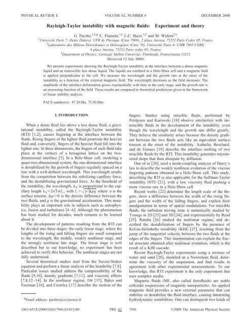
PHYSICAL REVIEW E VOLUME 62, NUMBER 6
DECEMBER 2000
Rayleigh-Taylor instability with magnetic fluids:
Experiment and theory
G. Pacitto, 1,2, * C. Flament, 1,2 J.-C. Bacri, 1,2 and M. Widom 3,1
1 Université Paris 7–Denis Diderot, UFR de Physique (Case 7008), 2 place Jussieu, 75251 Paris Cedex 05, France
2 Laboratoire des Milieux Désordonnés etHétérogènes (Case 78), Université Paris 6–UMR 7603 CNRS,
4 place Jussieu, 75252 Paris cedex 05, France
3 Department of Physics, Carnegie Mellon University, Pittsburgh, Pennsylvania 15213
Received 12 July 2000
We present experiments showing the Rayleigh-Taylor instability at the interface between a dense magnetic
liquid and an immiscible less dense liquid. The liquids are confined in a Hele-Shaw cell and a magnetic field
is applied perpendicular to the cell. We measure the wavelength and the growth rate at the onset of the
instability as a function of the external magnetic field. The wavelength decreases as the field increases. The
amplitude of the interface deformation grows exponentially with time in the early stage, and the growth rate is
an increasing function of the field. These results are compared to theoretical predictions given in the framework
of linear stability analysis.
PACS numbers: 47.20.Ma, 75.50.Mm
I. INTRODUCTION
When a dense fluid lies above a less dense fluid, a gravitational
instability, called the Rayleigh-Taylor instability
RTI 1,2, causes fingering at the interface between the
fluids. Rising fingers of the lighter fluid penetrate the heavier
fluid and, conversely, fingers of the heavier fluid fall into the
lighter one. In three dimensions, the fingers of each fluid take
place at the vertices of a hexagonal lattice on the twodimensional
interface 3. In a Hele-Shaw cell, modeling a
quasi-two-dimensional system, the one-dimensional interface
is destabilized by the growth of fingers regularly spaced on a
line with a well-defined wavelength. This wavelength results
from the competition between the stabilizing capillary force,
and the destabilizing gravitational force. At the threshold of
the instability, the wavelength, 0 is proportional to the capillary
length 0 2)l c , with l c /g where is the
surface tension, 0 is the density difference between the
two fluids, and g is the gravitational acceleration. This instability
plays an important role in subjects such as astrophysics,
fusion and turbulence 4–6. Although the phenomenon
has been studied for decades, much remains to be learned
about it.
The development of patterns resulting from the RTI can
be divided into three stages: the early linear stage, where the
lengths of the rising and falling fingers are small compared
to the wavelength, the middle, weakly nonlinear stage, and
the strongly nonlinear late stage. The linear stage is well
described but to our knowledge, no experiment has been
achieved to verify this behavior. The nonlinear stages are not
fully understood.
Several theoretical studies start from the Navier-Stokes
equation and perform a linear analysis of the instability 7,8.
Particular issues studied address the compressibility of the
fluids 9,10, density gradients 7,11, and viscosity effects
7,8,12–14. In the nonlinear regime, Ott 15, Baker and
Freeman 16, and Crowley 17 describe the motion of the
*Email address: pacitto@ccr.jussieu.fr
fingers. Studies using miscible fluids, performed by
Petitjeans and Kurowski 18 observe similarities with immiscible
fluids in the development of the instability, even
though the wavelength and the growth rate differ greatly.
They believe the similarity arises because the density gradient
between the two fluids acts like an equivalent surface
tension at the onset of the instability. Authelin, Brochard,
and de Gennes 19 describe the interface melting of two
miscible fluids by the RTI. This instability generates micronsized
drops that then dissipate by diffusion.
One of us 20, used a mode-coupling analysis of Darcy’s
law to describe the weakly nonlinear evolution of the viscous
fingering patterns obtained in a Hele-Shaw cell. This study,
describing the RTI is also applicable for the Saffman-Taylor
instability STI 21, with a low viscosity fluid pushing a
more viscous one in a Hele-Shaw cell.
Recent works 22 determine the length scale of the fingers,
show a difference between the width of the rising fingers
and the width of the falling fingers, and explain their
amalgamation in terms of spatial modulations. For miscible
fluids, the turbulent mixing zone is numerically studied by
Youngs in 2D 23 and 3D 24, and experimentally by Read
25. Ratafia 26 studied the nonlinear regime, and described
the destabilization of fingers by the presence of
Kelvin-Helmholtz instability KHI 27, resulting from the
jump of the tangential velocity between the two fluids at the
edges of the fingers. This interpretation can explain the fractal
structure obtained after nonlinear evolution, which is the
result of a KHI cascade.
Recent Rayleigh-Taylor experiments using a mixture of
water and sand 28, modeled as a Newtonian fluid, determine
the viscosity of the suspension, and find results in
agreement with other experimental measurements. To our
knowledge, this RTI experiment is the only experiment that
uses complex media.
Magnetic fluids MF, also called ferrofluids are stable
colloidal suspensions of magnetic nanoparticles. An applied
magnetic field provides a new external parameter that can
stabilize or destabilize the fluid interface, causing interesting
hydrodynamic instabilities. One can distinguish two kinds of
1063-651X/2000/626/79418/$15.00 PRE 62 7941 ©2000 The American Physical Society

7942 G. PACITTO, C. FLAMENT, J.-C. BACRI, AND M. WIDOM
PRE 62
instabilities in ferrofluids: static instabilities caused by the
magnetic field, which are not present in ordinary fluids; and
dynamic instabilities that appear or are modified by applied
fields.
The first static instability observed in MF is the peak instability
29. A static magnetic external field H ext applied
tangent to a free surface generally stabilizes the surface.
However, H ext applied normal to a horizontal surface causes
the peak instability to rise above a critical value of H ext .A
line in 2D or a lattice in 3D of spikes arises from the
competition between the destabilizing magnetic forces and
the stabilizing capillary and gravitational forces.
Now, let the MF be confined in a two-dimensional Hele-
Shaw cell. Another instability can appear if the external field
is applied in the direction perpendicular to the cell. This
phenomenon, called the labyrinthine instability 30,31, occurs
above a critical value of the applied field and with a
critical wavelength. The threshold value of H ext results from
a balance between the destabilizing magnetic dipole-dipole
repulsion and the stabilizing surface tension and possibly
gravity in a vertical cell.
MF can be used as a dynamic system if a time-dependent
magnetic field is applied. Different surface phenomena are
observed such as surface waves 32,33, the Faraday instability
34, or a period doubling in the case of the peak instability
35.
Hydrodynamic instabilities may occur when the MF
flows. For example, Saffman-Taylor fingering has been studied,
both experimentally and theoretically, with an MF. In
this configuration, the external magnetic field can be applied
normal to, or within the plane of the cell. The situation is
stabilizing if H ext is tangent to the interface within the plane
of the cell 36. Experiments performed with a field applied
in a direction perpendicular to a circular Hele-Shaw cell
show a destabilizing behavior 37.
The aim of this paper is to study the influence of a homogeneous
magnetic field applied perpendicular to a vertical
Hele-Shaw cell filled with a dense water-based ferrofluid
above a lighter oil. In a recent paper 38, one of us describes
theoretically the general viscous fingering pattern obtained in
this configuration. In this dynamic situation, the magnetic
force is added to the gravitational force to destabilize the
interface, while the capillary effects stabilize it.
II. LINEAR STABILITY ANALYSIS
Consider a vertical Hele-Shaw cell of gap h filled with oil
of density and viscosity at the bottom and an immiscible
MF of density and viscosity on top. We use a
coordinate system in which the Hele-Shaw cell lies parallel
to the xy plane, the y axis is vertically upward, and the z axis
is perpendicular to the Hele-Shaw cell. Gravity acts downward
parallel to the y axis and a uniform external magnetic
field H ext H ext ẑ, is parallel to the z axis see Fig. 1. We
present equations of motion and boundary conditions and
then we perform a linear stability analysis of these equations.
We show that both gravitational provided ) and
magnetic instabilities deform an initially flat interface.
To begin, we derive Darcy’s law for the flow of MF. The
analysis begins with the basic equation governing the threedimensional
fluid flow v (x,y,z), the Navier-Stokes equation
FIG. 1. The experimental setup consists in a cell located vertically
between two coils. The external magnetic field obtained is
horizontal and perpendicular to the cell. The cell that contains the
both liquids can be rotated around a horizontal axis.
Dv
Dt pg v f m .
From this equation, we derive Darcy’s law assuming sufficiently
high viscosity so that the flow velocity is small, so
the inertial term on the left-hand side may be neglected. The
idea is to average Eq. 1 over the gap, resulting in a 2D flow
equation for the gap-averaged velocity u . The gap average of
the three-dimensional pressure gradient yields a twodimensional
gradient of the gap-averaged pressure, which we
continue to represent as p . As is usual in derivations of
Darcy’s law, the gap average of the viscous drag force, subject
to no-slip boundary conditions imposed at zh/2, is
(12/h 2 )u .
The final term in Eq. 1, f m 0 (M • )H , represents the
magnetic body force on a fluid element, neglecting compressibility
and self-induction of the fluid 39. In this approximation,
M is constant and parallel to z, and the gap
average of f m reduces to ( 0 M/h)H(x,y,h/2)H(x,y,
h/2). Because the applied field H ext is spatially uniform,
it drops out of this difference and the magnetic force arises
entirely from the demagnetizing field H d H H ext caused
by the surface magnetic poles. Express the demagnetizing
field as the gradient of a magnetic scalar potential, H d
(x,y,z), and take as an odd function of z. The gap
average of the magnetic force is f m
(2 0 M/h) (x,y,h/2), where now the gradient acts only
on x and y coordinates 40.
Collect all averaged terms and isolate the velocity u on
the left-hand side,
1
12
2M
h 2 u pgŷ 0
h x,y. 2
Here all vectors lie in the xy plane, and the scalar potential
(x,y)(x,y,h/2) is evaluated at the top plate. Further

PRE 62 RAYLEIGH-TAYLOR INSTABILITY WITH MAGNETIC ...
7943
simplification of Darcy’s law 2 occurs if we exploit the
irrotational flow to introduce the velocity potential u
so that
12
2M
h 2 pgy 0 x,y. 3
h
Now we apply Darcy’s law 3 within each fluid evaluated
at the interface between the two fluids, y(x). Subtract
Eq. 3 for the oil fluid from the same equation for
MF fluid and find
A
2
2
h 2
2M
12
p
p 0
h
h2 g
12
for the viscosity contrast A( )/( ). The
pressure jump across the interface, p p , is the surface
tension times the mean interface curvature . For a thin
gap h, we need only consider the curvature of (x), which
we may approximate 2 /x 2 for the purpose of linear
stability analysis 38.
Represent the net perturbation (x,t) in the form of a
Fourier mode
x,t k tcoskx.
The velocity potentials must obey Laplace’s equation
2 0, because the fluids are incompressible. The boundary
conditions at y→, so that 0. We give the
appropriate wavevector and phase to be consistent with the
perturbation . The general velocity potentials obeying these
requirements are
x,y,t k expkycoskx.
In order to substitute expansions 6 into the equation of
motion 4, we need to evaluate them at the perturbed interface.
To first order in the perturbation, it suffices to simply
set y0 in Eq. 6.
To close Eq. 4 we need additional relations expressing
the velocity potentials in terms of the perturbation amplitudes.
To find these, consider the kinematic boundary condition
that the interface moves according to the local fluid
velocities. To first order in , we simply note /t
i /y 38. Substituting Eq. 6 for and Fourier
transforming yields ˙ kk k k k . Then Eq. 4 reads
1
k
k
t h 2
2M
12
k 2
k 0
h
h2 g
12 k
k
To obtain the Fourier transform of the magnetic scalar
potential, k , we write the magnetic scalar potential
4
5
6
7
x,y M 4
dx
x
1
xx 2 yy 2 h 2.
dy
1
xx 2 yy 2
The expansion of „x,(x)… to first order in is
x 0 M 1
dx
4
2
1
xx 2 xx 2 h
xx
and its Fourier transform k 2MJ(kh) k , where
Jxlnx/2K 0 xC Euler
8
9
10
with where K 0 a Bessel function and C Euler 0.5772 ... is
the Euler constant 41.
Inserting k into Eq. 7 for the growth of the cosine
mode, the differential equation of the interface is
where
˙ kk k ,
kkV c B G 2B M Jkhkh 2
11
12
is the linear growth rate multiplying the first-order term in
with V c /12( ) as the capillary velocity, B G
( )gh 2 / the gravitational Bond number, and
B M
0
4 2M 2 h
is the magnetic Bond number. An asymptotic expression for
kh1 that is more convenient for the data analysis can be
obtained by expanding J(kh) for small kh 42:
Jkh kh2
1C
4
Euler lnkh/2.
III. EXPERIMENTAL SETUP
13
The experimental geometry is sketched in Fig. 1. The cell
is located in a gap between two coils in the Helmholtz configuration
to achieve good axial homogeneity for the magnetic
field H ext . The radial homogeneity of the field is better
than 3%. The amplitude of the external field is nearly constant.
The cell is mounted so it can be rotated around the x
axis, which passes through the middle of the gap.
We use an ionic magnetic fluid made of cobalt ferrite
particles (CoFe 2 O 4 ) dispersed in a mixture of water and
glycerol. This MF is synthesized by Neveu 43 following
the Massart’s method 44. The magnetization of the MF as a
function of H ext is obtained by the use of a calibrated
fluxmeter.
The rectangular cell consists of two parallel plates made
of altuglass Plexiglas with a spacing between the two plates
of h500 m. The cell is initially filled with an oil White
Spirit or WS of low density compared to the MF that wets

7944 G. PACITTO, C. FLAMENT, J.-C. BACRI, AND M. WIDOM
PRE 62
FIG. 2. Several pictures of the destabilizing MF-WS interface
for different times a t0; b t5 s; c t8 s; d t11 s for
H ext 7.9 kA/m. The gray bar equals 1 cm.
the altuglass walls. A thin film of micron width of WS
separates the MF from the walls, avoiding pinning of the
MF-WS contact line on the walls.
The mass density of MF is 168685 kg m 3 , compared
to 800 kg m 3 for WS. The dynamic viscosity of
the MF is 0.14 kg m 1 s 1 at room temperature. The
viscosity of the WS is two orders of magnitude lower, so we
may take 0.
Image processing is used to measure the wavelength and
the growth increment. The images are recorded by a CCD
camera charge-coupled device and digitized by an acquisition
card in a computer. We use the public domain software
NIH Image 45 to analyze the images.
IV. RESULTS
A. Wavelength measurements
The experiments are conceptually simple: the cell is
placed vertically with the heavier liquid MF below. We
rotate the cell by 180° around the x axis and apply the magnetic
field. The selected wavelength depends on how and
when the magnetic field is applied. If H ext is applied during
the rotation, we get a different measurement than if H ext is
switched on at the end of the rotation. The response of the
MF-WS interface to the magnetic field is usually much faster
than its response to a gravitational field. That is, a longer
time is needed to observe the classical RTI without an external
magnetic field than to observe the labyrinthine instability
30,31. IfH ext is applied during rotation when the cell is
momentarily horizontal, the normal field instability 29 appears
before the RTI. To avoid these difficulties, we apply
the field only after the rotation is complete, but before the
RTI appears. The duration of rotation is about 1 s, and the
time constant for ramping up the magnetic field is less than 1
s.
We collected data for 13 different values of H ext , with
two independent runs for each value of H ext . The wavelength
0 2/k 0 , is measured at the onset of the instability
until the amplitude of the interface deformation remains
small: k 0 0.1. We compared two different methods: a FFT
of the interface gives the fundamental mode k 0 , a direct
measurement of the average peak to peak distance gives 0 .
In the second approach, we reject the peaks located close to
the edges of the cell, and we omit certain peaks that are
dominated by others ‘‘finger competition’’. Both methods
give similar results within the errors bars.
FIG. 3. Several destabilizing interfaces for different values of
the applied field a H ext 4.1 kA/m and t8 s; b H ext
11.9 kA/m and t9 s; c H ext 17.8 kA/m and t6 s; H ext
31.6 kA/m and t1 s. The gray bar equals 1 cm.
Figure 2 displays a sequence of pictures of the destabilizing
MF-WS interface for H ext 7.9 kA/m. A comparison of
interfaces for different values of the external field is shown
in Fig. 3. Both the wavelength and the width of the MF
fingers decrease as H ext increases. The experimental values
of 0 as a function of the external field H ext are reported in
Fig. 4.
To compare experimentally observed wavelengths with
the linear stability analysis, consider the growth rate, (k).
Maximizing expression 12 for (k) versus the wavevector,
gives the fastest growing mode k 0 :
k
0⇔ 0 2
.
k
kk 0 0
We get the following nonalgebraic equation:
B G
4 2 x 0 2 B M a 3 2 lnx 0 30,
14
with, a1 3 2 C Euler 3 2 ln()0.79, and x 0 0 /h. To
determine the value of
FIG. 4. Wavelength as a function of the external applied field
H ext . Experimental data are measured by the direct peak-to-peak
method, at the onset of the instability.

PRE 62 RAYLEIGH-TAYLOR INSTABILITY WITH MAGNETIC ...
7945
B M 0 2M 2 h
4
for a given value of H ext , we need to know the MF-WS
surface tension . The value of can be deduced from the
wavelength at the onset of the RTI with H ext 0 using formula
12. Wefind8.63.8 mN m 1 by this method. We
can also determine the value of from the wavelength at the
threshold of the normal field instability, which is linked with
the capillary length 46. This method yields 12.0
1.3 mN m 1 , which is closed to the previous value. The
value of the magnetization M(H ext ) is directly deduced from
the magnetization curve of the MF. Taking the latter value of
, we deduce a capillary length l c 0.12 cm, and the gravitational
Bond number B G 0.18. The roots of Eq. 14 are
reported in Fig. 4 for comparison with the experimental data.
Both are qualitatively coherent. We get a good agreement for
low values and high values of H ext . The discrepancy for the
intermediate values should result from the omission of the
demagnetizing effect in the magnetic forces.
To take into account this demagnetizing effect, we have to
consider an infinite plane with an external field applied perpendicular
to the plane. The demagnetizing factor is equal to
D1. Consequently, the local field is: H H ext DM
H ext M . The magnetization M , is linked to the local
field by the relation M H , it leads to M (/1
)H ext . A local susceptibility can be determined by the
use of the magnetization curve: (H ext )M(H ext )/H ext 47,
and subsequently a magnetic Bond number including the demagnetizing
effect is
B M 0 2M 2 h
4
We can calculate the contribution of the demagnetizing effects
to the theoretical roots. The results are also shown in
Fig. 4. The experimental values are between the theoretical
predictions D0 demagnetizing effects neglected and D
1 demagnetizing effects maximized. An exact calculation
would have to deal with the nonuniform fringe fields at
the edge of a paramagnetic slab.
B. Growth rates
Now, let us study the growth rate of the instability. We
measure the length of the falling fingers, and divided by
0 (tt 0 ); t 0 corresponds to the first time where the interface
deformation is detectable and is actually given by the
resolution of the video recorder. We use a direct measurement
of the length instead of a Fourier analysis since it gives
results with a huge scattering. Moreover, we have checked
that both methods give similar results within the error bars
for the wavelength at the onset of the RTI. Plotting this relative
depth to which the instability penetrates the lighter fluid
as a function of time, we can clearly separate two distinct
stages Fig. 5.
Just after the onset of the instability, when the amplitude
of the growth the length of the spikes is small compared to
the wavelength, we see an exponential growth over time.
This occurs for all values of the external applied field. We
FIG. 5. Growth rates for H ext 23.6 kA/m in the exponential
regime and in the linear regime shown in the inset as a function of
time.
observe an augmentation in the growth rate values as the
field increases, as is predicted by the linear analysis given by
the formula 12. In this equation, the growth rate is a function
of H ext and also a function of x 0 . As we have seen in
the previous part, x 0 is an implicit function of H ext , and we
cannot find an explicit expression of (H ext ). Nevertheless,
Eq. 12 can be written
*
B
˜ M
15
with the growth rate for the mode of wavelength 0 hx 0 in
the absence of magnetic field
* b x 0
B G
4 2 x 0
2
and a characteristic inverse of time
˜ b
2x 0
3 aln x 0 .
We define b2 3 /3 h and a1C Euler ln
0.72, and x 0 is defined previously.
If we insert the theoretical values of the wavelength x 0 th ,
in the expressions of * and ˜ we can compare the theoretical
linear analysis to the experimental measurements of
exp .
These experimental results of the growth rate exp measured
near the onset of the instability for different values of
the external applied field are shown in Fig. 6, where we plot
( exp *)/˜ versus the magnetic Bond number. The theoretical
continuous line results from the linear analysis Eq.
15 and is the first bisectrix of the Fig. 6. The experimental
results are below the theoretical curve, but are included in
the error bars. These experimental uncertainties are large due
to the difficulty of measuring the amplitude .
To reduce the systematic discrepancy between the two
curves, we can, as with the wavelength treatment, take into
account the demagnetizing field effect. The plot of ( exp
*)/˜ versus B M is also reported in Fig. 6. In contrast to
the previous case, the data are above the first bisectrix. Since

7946 G. PACITTO, C. FLAMENT, J.-C. BACRI, AND M. WIDOM
PRE 62
FIG. 6. Magnetic field dependence of the growth rate; black
circles represent the experimental data see text without demagnetizing
effects; white squares maximize the demagnetizing effects in
the expression of the magnetic Bond number.
we have crudely included the demagnetizing fields through a
demagnetizing factor D1, the demagnetizing effects are
naturally overestimated, and this explains the intermediate
position of the theoretical prediction between the points with
D0 and the ones with D1. A fully three-dimensional
calculation is needed to properly treat the demagnetization
fields at the MF-WS interface.
After the initial exponential growth of the disturbances,
we enter a new growth regime shown in the inset of Fig. 5. A
linear growth is observed for each value of the applied magnetic
field. This behavior is observed for long times, up to
the secondary instabilities, where the finger tips split and
start to compete with each other. As the magnetic field increases,
we observe an increase in the linear coefficient. For
example, for H ext 0, we get 0 1.92.0(tt 0 ), and
for H ext 39.3 kA/m, we get 0 10.820.1(tt 0 ).
Saturation of the exponential growth is predicted by weakly
nonlinear analysis 38. Crossover from exponential to linear
has been found in numerical simulations for nonmagnetic
fluids 51.
C. Far from the threshold
This study emphasized the downward propagating MF
fingers, but upward fingers made of WS also exist. As a
matter of fact, the heavier liquid, i.e., the MF, falls down due
to the buoyancy forces and consequently, the lighter liquid
that is the less viscous fluid has to penetrate into the viscous
one. A finger of WS grows between each spike of MF. These
WS fingers rise like the ST finger propagating in a narrow
channel 21. In fact, both instabilities RTI and STI can be
described by the same set of equations 38. The width of the
WS fingers is greater than the MF fingers, but a common
feature is that the width is a decreasing function of the external
magnetic field. Such a symmetry breaking of the interface
is related to the viscosity contrast between MF and
WS 38.
The tip of the WS fingers splits into two fingers the socalled
‘‘tip-splitting’’ phenomenon and the angle between
these new fingers is roughly equal to 90°. The evolution of
the system exhibits a cascade of tip splitting: each new finger
divides itself into two fingers that destabilize themselves
while they remain upward. Let us notice that the finger
FIG. 7. Pictures of the RTI far from the threshold see text and
for high value of the applied field: H ext 40 kA/m. The black bar
equals 1 cm.
changes its direction slightly after each tip splitting: it seems
to undulate like a narrow finger confined in a channel in the
‘‘oscillating-tip’’ regime 48. No other secondary instability
such as the ‘‘side-branching’’ phenomenon is observed. The
tip-splitting cascades acting on a finger give a pattern that
looks like a tree as it is illustrated in Fig. 7. This pattern is
somewhat similar to the radial viscous fingering obtained
with the STI 37 with the difference that the system is anisotropic
due to the gravity field.
The MF fingers always remain stable because the viscosity
contrast is opposite a viscous fluid penetrating a less
viscous one is stable situation. When the MF fingers are
sufficiently far from each other and for high values of the
magnetic field, a bending instability occurs 49. When the
distance between the fingers is comparable to the finger
width, long range magnetic interactions between fingers are
visible: they undulate together for high magnetic field in the
same manner than the MF parallel stripes in the bending
instability 50. Finally, the pattern is very non-symmetric
Fig. 7b because of all these features. For high amplitudes
of the external field and at long times the top of the cell
becomes a labyrinthine and the bottom is rather well organized
as the MF smectic 50.
At very long times, the MF accumulates in the bottom of
the cell, displacing the WS to the top. The limiting pattern is
a conventional MF labyrinth 39 with a reservoir MF at the
bottom of the cell Fig. 8. We investigated whether a hierarchical
dynamical behavior 52 emerges because of the
treelike structure of highly bifurcated fingers of WS. Retraction
of bifurcated fingers cannot occur because their points of
bifurcation represent points of force balance and are therefore
immobile. To undo a bifurcation requires retraction of at
least one of the branches inset of Fig. 8. However, each
branch may itself be bifurcated, further slowing down the
pattern evolution. Only at finger tips are forces unbalanced
and dynamics unfrozen. Hierarchically constrained dynamics
leads to glassy behavior 52. A Kohlrausch stretched expo-

PRE 62 RAYLEIGH-TAYLOR INSTABILITY WITH MAGNETIC ...
7947
V. CONCLUSION
FIG. 8. Final state of the RTI at high fields H ext 40 kA/m. In
the inset, intermediate stage evolution of the RTI at long time: a
Arrow points to branched finger about to disappear. b 0.5 s later,
one branch has retracted. c 4 s later, the entire finger disappears.
The black bar equals 1 cm.
nential law should govern the evolution in this regime. However,
our experiments are consistent with a conventional exponential
behavior, at least at short times. In particular, we
measured the total interface contour length as a function of
time. Over a period of 120 s it fits well to an exponential
relaxation with a time constant of 25 s.
We perform the Rayleigh-Taylor instability experiment
using magnetic fluid. Near the onset of the instability, to
describe the pattern, we measure, for different values of the
magnetic field, the wavelength and the growth rate of the
observed fingers. The magnetic field destabilizes the interface,
decreasing the wavelength and increasing the growth
rate as it is predicted by the linear analysis of the ferrohydrodynamics
equations. We get a good agreement between
experiments and theory. At long times, a comparison with
numerical simulations for different values of the fields will
be of great interest. Other experiments can be performed
using a magnetic field applied parallel to the interface in
order to stabilize the interface.
ACKNOWLEDGMENTS
We are greatly indebted to Sophie Neveu for providing us
with the magnetic fluid and Patrick Lepert for building the
experimental device. We acknowledge useful discussions
with Jose Miranda and support by the National Science
Foundation Grant No. DMR-9732567.
1 Lord Rayleigh, Scientific Papers II Cambridge University
Press, Cambridge, England, 1900, p. 200.
2 G. I. Taylor, Proc. R. Soc. London, Ser. A 201, 192 1950.
3 M. Fermigier, L. Limat, J.-E. Weisfreid, P. Boudinet, and C.
Quilliet, J. Fluid Mech. 236, 349 1992.
4 D. H. Sharp, Physica D 12, 31984.
5 L. Smarr, J. R. Wilson, R. T. Barton, and R. L. Bowers, Astrophys.
J. 246, 515 1981.
6 H. J. Kull, Phys. Rep. 206, 197 1991.
7 S. Chandrasekhar, Hydrodynamic and Hydromagnetic Stability
Oxford University Press, Oxford, 1961, Chap. X.
8 R. Menikoff, R. C. Mjolsness, D. H. Sharp, C. Zemach, and B.
J. Doyle, Phys. Fluids 21, 1674 1978.
9 M. Mitchner and R. K. M. Landshoff, Phys. Fluids 7, 862
1964.
10 M. S. Plesset and D-Y. Hsieh, Phys. Fluids 7, 1099 1964.
11 R. LeLevier, G. J. Lasher, and F. Bjorklund, Lawrence Livermore
Laboratory Report No. UCRL-4459, 1955 unpublished.
12 R. Menikoff, R. C. Mjolsness, D. H. Sharp, and C. Zemach,
Phys. Fluids 20, 2000 1977.
13 K. O. Mikaelian, Phys. Rev. E 47, 375 1993.
14 A. Elgowainy and N. Ashgriz, Phys. Fluids 9, 1635 1997.
15 E. Ott, Phys. Rev. Lett. 29, 1429 1972.
16 L. Baker and J. R. Freeman, Sandia National Laboratories Report
No. Sand80-0700, 1980 unpublished.
17 W. P. Crowley, Lawrence Livermore Laboratory Report No.
UCRL-72650, 1970 unpublished.
18 P. Petitjeans and P. Kurowski, C. R. Acad. Sci. Paris 325, 587
1997.
19 J.-R. Authelin, F. Brochard and P.-G. de Gennes, C. R. Acad.
Sci. Paris 317, 1539 1993.
20 J. A. Miranda and M. Widom, Int. J. Mod. Phys. B 12, 931
1998.
21 P. G. Saffman and Sir G. I. Taylor, Proc. R. Soc. London, Ser.
A 245, 312 1958.
22 S. I. Abarzhi, Phys. Fluids 11, 940 1999.
23 D. L. Youngs, Physica D 12, 321984.
24 D. L. Youngs, Phys. Fluids A 3, 1312 1991.
25 K. I. Read, Physica D 12, 451984.
26 M. Ratafia, Phys. Fluids 16, 1207 1973.
27 P. Gondret and M. Rabaud, Phys. Fluids 9, 3267 1997.
28 A. Lange, M. Schröter, M. A. Scherer, A. Engel, and I. Rehberg,
Eur. Phys. J. B 4, 475 1998.
29 M. D. Cowley and R. E. Rosensweig, J. Fluid Mech. 30, 671
1967.
30 A. Cebers and M. M. Maiorov, Magn. Gidrodin. 1, 127 1980;
3, 151980.
31 R. E. Rosensweig, M. Zahn, and R. Shumovich, J. Magn.
Magn. Mater. 39, 127 1983.
32 T. Mahr and I. Rehberg, Phys. Rev. Lett. 81, 891998.
33 J. Browaeys, J.-C. Bacri, C. Flament, S. Neveu, and R. Perzynski,
Eur. Phys. J. B 9, 335 1999.
34 J.-C. Bacri, A. Cebers, J.-C. Dabadie, S. Neveu, and R.
Perzynski, Europhys. Lett. 27, 437 1994.
35 J.-C. Bacri, U. d’Ortona, and D. Salin, Phys. Rev. Lett. 67, 50
1991.
36 M. Zahn and R. E. Rosensweig, IEEE Trans. Magn. 16, 275
1980.
37 C. Flament, G. Pacitto, J.-C. Bacri, I. Drikis, and A. Cebers,
Phys. Fluids 10, 2464 1998.
38 M. Widom and J. Miranda, J. Stat. Phys. 93, 411 1998.
39 R. W. Rosensweig, Ferrohydrodynamics, Cambridge University
Press, Cambridge, England, 1985.
40 D. P. Jackson, R. E. Goldstein, and A. O. Cebers, Phys. Rev. E
50, 298 1994.
41 A. O. Cebers, Magnetohydrodynamics 16, 236 1980.
42 Handbook of Mathematical Functions, edited by M. Abrahamovitz
and I. A. Stegun Dover, New York, 1965, p. 375.
43 S. Neveu from the Laboratoire des Liquides Ioniques et Interfaces
Chargées, located at University Paris 6.

7948 G. PACITTO, C. FLAMENT, J.-C. BACRI, AND M. WIDOM
PRE 62
44 R. Massart, IEEE Trans. Magn. 17, 1247 1981.
45 NIH Image by Wayne Rasband, National Institutes of Health
available at http://rsb.info.nih.gov/nih-image/.
46 C. Flament, S. Lacis, J.-C. Bacri, A. Cebers, S. Neveu, and R.
Perzynski, Phys. Rev. E 53, 4801 1996.
47 We use (H ext )M/H ext instead of M/H because it is not
possible to measure directly the internal magnetic field.
48 Y. Couder, N. Gerard, and M. Rabaud, Phys. Rev. A 34, 5175
1986.
49 J.-C. Bacri, A. Cebers, C. Flament, S. Lacis, R. Melliti, and R.
Perzynski, Prog. Colloid Polym. Sci. 98, 301995.
50 C. Flament, J.-C. Bacri, A. Cebers, F. Elias, and R. Perzynski,
Europhys. Lett. 34, 225 1996.
51 G. Tryggvason and H. Aref, J. Fluid Mech. 154, 287 1985.
52 R. G. Palmer, D. L. Stein, F. Abrahams, and P. W. Anderson,
Phys. Rev. Lett. 53, 958 1984.