Stochastic Calculus, Week 9 Applications of risk-neutral valuation

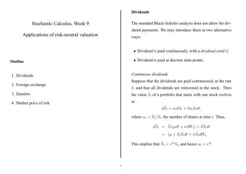
Dividends
Stochastic Calculus, Week 9
Applications of risk-neutral valuation
The standard Black-Scholes analysis does not allow for dividend
payments. We may introduce them in two alternative
ways:
• Dividend is paid continuously, with a dividend yield δ;
Outline
• Dividend is paid at discrete time points.
1. Dividends
2. Foreign exchange
3. Quantos
4. Market price of risk
Continuous dividends
Suppose that the dividends are paid continuously at the rate
δ, and that all dividends are reinvested in the stock. Then
the value ˜S t of a portfolio that starts with one stock evolves
as
d ˜S t = a t dS t + δa t S t dt,
where a t = ˜S t /S t , the number of shares at time t. Thus,
d ˜S t = ˜S t (µdt + σdW t )+δ ˜S t dt
= (µ + δ) ˜S t dt + σ ˜S t dW t .
This implies that ˜S t = e δt S t , and hence a t = e δt .
1

A strategy (φ t ,ψ t ) in terms of (S t ,B t ) may be written as
a corresponding strategy (˜φ t ,ψ t ) in terms of ( ˜S t ,B t ), with
˜φ t = e −δt φ t . The self-financing restriction now is (with V t =
˜φ t ˜St + ψ t B t )
dV t
= ˜φ t d ˜S t + ψ t dB t
= φ t dS t + φ t δS t dt + ψ t dB t .
The essential point is that, whereas the replicating portfolio
is in terms of ˜S t , the derivative is in terms of S t . Note that
the measure Q which makes ˜Z t = Bt
−1 ˜S t a martingale, does
not make Bt
−1 S t a martingale.
We find
This yields, via risk-neutral valuation:
• The forward price of S t : setting e −r(T −t) E Q [(S T −
F t )|F t ]=0and solving for F t gives
F t = e (r−δ)(T −t) S t .
• The price of a call option struck at K. Following the
same steps as in the standard Black-Scholes model, we
find
V t = e −r(T −t) E Q [(S T − K) + |F t ]
= e −δ(T −t) S t Φ( ˜d 1 ) − e −r(T −t) KΦ( ˜d 2 )
= e
{F −r(T −t) t Φ( ˜d 1 ) − KΦ( ˜d
}
2 )
d ˜Z t = (µ + δ − r) ˜Z t dt + σ ˜Z t dW t
= σ ˜Z t d ˜W t ,
where ˜W t = W t + γt, with γ = µ + δ − r , which is a
σ
Brownian motion under the measure Q defined by dQ/dP =
exp(−γW T − 1 2 γ2 T ). Hence
dS t = (r − δ)S t dt + σS t d ˜W t ,
= S 0 exp
([r − δ − 1 2 σ2 ]t + σ ˜W
)
t
S t
with
˜d 1,2 = log(S t/K)+[(r − δ) ± 1 2 σ2 ](T − t)
σ √ T − t
= log(F t/K) ± 1 2 σ2 (T − t)
σ √ .
T − t
2

Discrete dividends
When dividends are paid at discrete time points T 1 ,...,T n ,
then the stock goes ex-dividend, which means its price falls
instantaneously by the amount of the dividend. When these
dividends are immediately reinvested, the value ˜S t of that
strategy of course does not display these discontinuities; i.e.,
we simply may assume
d ˜S t = µ ˜S t dt + σ ˜S t dW t .
(Note: µ here should be compared with µ + δ in the continuous
dividend model).
When the dividend payments are δS t , we obtain
S t =(1− δ) n[t] ˜St ,
where n[t] is the number of dividend payments made by
time t.
This implies
F t =(1− δ) n[T ]−n[t] e r(T −t) S t ,
Foreign exchange
Let C t denote the exchange rate, in US dollar per pound
sterling. We’ll assume a geometric Brownian motion for
C t :
dC t = µC t dt + σC t dW t .
Next, consider a US cash bond B t = e rt and a UK cash bond
D t = e ut ; i.e., the interest rates r and u may be different.
From the perspective of the US investor, there are two assets:
the domestic cash bond with price B t , and the foreign
cash bond with price S t = C t D t . Note that the latter is a
risky asset; its SDE is
dS t = C t dD t + D t dC t
= (µ + u)S t dt + σS t dW t
= rS t dt + σS t d ˜W t ,
where ˜W t = W t + γt, γ = µ + u − r . This again defines
σ
Q, the risk-neutral measure.
and the value of a call option remains the same in terms of
F t .
3

Notice that under this measure,
E Q [C T |F t ] = e −uT E Q [S T |F t ]
= e −uT e r(T −t) S t
= e (r−u)(T −t) C t ,
which yields the uncovered interest rate parity:
(r − u)(T − t) = log E Q[C T |F t ]
,
C t
where the right-hand side is the conditionally expected continuous
depreciation.
The forward exchange rate (for delivery at time T ) F t should
solve
e −r(T −t) E Q [(C T − F t )|F t ]=0,
(
and since C T = C t exp [r − u − 1 2 σ2 ](T − t)+σ[ ˜W T − ˜W
)
t ] ,
this will yield
F t = e (r−u)(T −t) C t ,
which gives the covered interest rate parity:
Again, the value of a call option on the exchange rate struck
at K is the same as before, when expressed in terms of F t .
Change of numeraire
The entire analysis could be repeated from the perspective
of the UK investor, who has the choice between a sterling
cash bond D t and the sterling value of a dollar cash bond,
˜S t = Ct
−1 B t . The discounted price then is Dt
−1 Ct −1 B t =
Z −1
t
, where Z t = Bt
−1 S t . The martingale measure is not
the same as before: a measure which makes Z t a martingale
does not make Zt
−1 a martingale. However, the prices and
hedge ratios are the same, regardless of the choice of the
measure.
Similarly, in the standard Black-Scholes model we may also
work with a measure Q ∗ which makes St
−1 B t a martingale.
The important thing is to make relative prices martingales –
the choice of the numeraire is not important.
(r − u)(T − t) = log F t
C t
.
4

Quantos
Quantos are derivatives which have a payoff in another currency
than the underlying asset, using a fixed, prespecified
exchange rate ¯C (e.g., one dollar per pound sterling). For
example, when S t is a sterling stock price and K is a corrresponding
strike price, then a quanto call has the dollar
payoff
¯C(S T − K) + .
In order to price such a derivative, one has to set up a joint
process for (S t ,C t ), which is a vector diffusion with two
independent Brownian motions (W 1 (t),W 2 (t)):
dS t
= µdt + σ 1 dW 1 (t),
S t
dC t
C t
= νdt + σ 2 dW ∗ 2 (t)
= νdt + ρσ 2 dW 1 (t)+ √ 1 − ρ 2 σ 2 dW 2 (t),
where W2 ∗ (t) = ρW 1 (t) + √ 1 − ρ 2 W 2 (t) is a standard
Brownian motion, which has correlation ρ with W 1 (t), i.e.,
E P [W 1 (t)W2 ∗ (t)] = ρt.
The equivalent martingale measure now should turn both
dollar assets Bt
−1 C t S t and Bt
−1 C t D t into martingale, which
now involves a vector γ =(γ 1 ,γ 2 ) ′ , with
dQ
dP = exp ( −γ ′ W T − 1 2 γ′ γT ) ,
where W T = (W 1 (T ),W 2 (T )) ′ . The actual definition of
γ follows from deriving the SDE for the discounted dollar
assets and setting the drifts to zero.
Note that ¯CSt is not a tradable dollar asset; hence its discounted
value need not be a martingale. In fact its drift is
(u − ρσ 1 σ 2 ) ¯CS t dt, which in general does not equal r ¯CS t dt.
It can be derived that the dollar forward price on ¯CS t will
be
F Qt = ¯C exp(−ρσ 1 σ 2 [T − t])F t ,
where F t is the sterling forward price. The quanto call value
then is the usual, with F t replaced by F Qt , K replaced by
¯CK, and σ replaced by σ 1 .
5

Market price of risk
The fundamental theorem of asset pricing states that the absence
of arbitrage opportunities is equivalent to the existence
of a measure Q under which all asset prices relative
to some numeraire are martingales. The equivalent martingale
measure is unique if markets are complete, i.e., if any
claim is replicable.
Note that only tradable asset need to be martingales under
Q; the previous examples all had a payoff in terms of a nontradable
asset, which was an explicit function of another
tradable.
The existence of Q implies a common market price of risk
γ t , which determines the change of measure via the CMG
theorem. For example, if two tradable asset prices S 1 (t) and
S 2 (t) are driven by the same Brownian motion W t :
then
dS 1 (t) = µ 1t S 1 (t)dt + σ 1t S 1 (t)dW t ,
dS 2 (t) = µ 2t S 2 (t)dt + σ 2t S 2 (t)dW t ,
γ t = µ 1t − r t
σ 1t
= µ 2t − r t
σ 2t
,
where r t is the risk-free interest rate. In models with more
than one driving Brownian motion, there is a vector of market
prices of risk, one for each source of risk (i.e., each
Brownian motion).
Exercises
1. Consider a bivariate geometric Brownian motion of the
form
dS 1 (t) = S 1 (t) {µ 1 dt + σ 11 dW 1 (t)+σ 12 dW 2 (t)} ,
dS 2 (t) = S 2 (t) {µ 2 dt + σ 21 dW 1 (t)+σ 22 dW 2 (t)} ,
where W 1 (t) and W 2 (t) are independent Brownian motions,
and µ i and σ ij are constants, i, j = 1, 2. Find
the vector γ of market prices of risks, and check that
e −rt S 1 (t) and e −rt S 2 (t) are both martingales under the
measure Q defined by this γ.
2. Suppose that S 1 and S 2 are geometric Brownian motions,
driven by the same Brownian motion W t . Show that if
both are tradable asset prices, but with a different market
price of risk, then an arbitrage opportunity exists.
6