Assignment 2 for Stochastic Calculus
Assignment 2 for Stochastic Calculus
Assignment 2 for Stochastic Calculus
You also want an ePaper? Increase the reach of your titles
YUMPU automatically turns print PDFs into web optimized ePapers that Google loves.
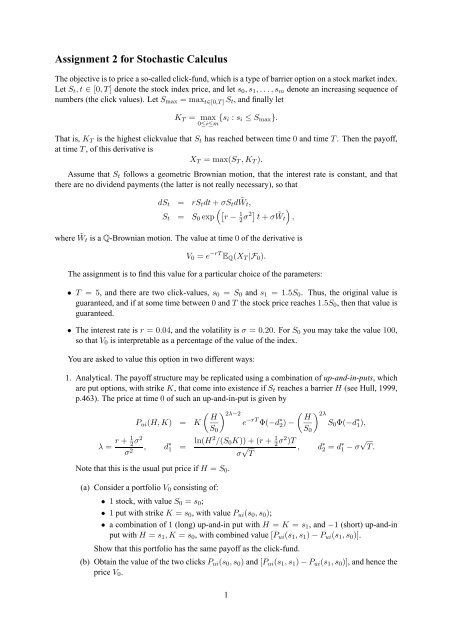
<strong>Assignment</strong> 2 <strong>for</strong> <strong>Stochastic</strong> <strong>Calculus</strong><br />
The objective is to price a so-called click-fund, which is a type of barrier option on a stock market index.<br />
Let S t ,t ∈ [0,T] denote the stock index price, and let s 0 ,s 1 ,...,s m denote an increasing sequence of<br />
numbers (the click values). Let S max = max t∈[0,T ] S t , and finally let<br />
K T = max<br />
0≤i≤m {s i : s i ≤ S max }.<br />
That is, K T is the highest clickvalue that S t has reached between time 0 and time T . Then the payoff,<br />
at time T , of this derivative is<br />
X T = max(S T ,K T ).<br />
Assume that S t follows a geometric Brownian motion, that the interest rate is constant, and that<br />
there are no dividend payments (the latter is not really necessary), so that<br />
dS t = rS t dt + σS t d ˜W t ,<br />
( [r<br />
S t = S 0 exp −<br />
1<br />
2 σ2] t + σ ˜W<br />
)<br />
t ,<br />
where ˜W t is a Q-Brownian motion. The value at time 0 of the derivative is<br />
V 0 = e −rT E Q (X T |F 0 ).<br />
The assignment is to find this value <strong>for</strong> a particular choice of the parameters:<br />
• T =5, and there are two click-values, s 0 = S 0 and s 1 =1.5S 0 . Thus, the original value is<br />
guaranteed, and if at some time between 0 and T the stock price reaches 1.5S 0 , then that value is<br />
guaranteed.<br />
• The interest rate is r =0.04, and the volatility is σ =0.20. ForS 0 you may take the value 100,<br />
so that V 0 is interpretable as a percentage of the value of the index.<br />
You are asked to value this option in two different ways:<br />
1. Analytical. The payoff structure may be replicated using a combination of up-and-in-puts, which<br />
are put options, with strike K, that come into existence if S t reaches a barrier H (see Hull, 1999,<br />
p.463). The price at time 0 of such an up-and-in-put is given by<br />
P ui (H, K) = K<br />
( H<br />
S 0<br />
) 2λ−2<br />
e −rT Φ(−d ∗ 2) −<br />
( H<br />
S 0<br />
) 2λ<br />
S 0 Φ(−d ∗ 1),<br />
λ = r + 1 2 σ2<br />
σ 2 , d ∗ 1 = ln(H2 /(S 0 K))+(r + 1 2 σ2 )T<br />
σ √ , d ∗ 2 = d ∗ 1 − σ √ T .<br />
T<br />
Note that this is the usual put price if H = S 0 .<br />
(a) Consider a portfolio V 0 consisting of:<br />
• 1 stock, with value S 0 = s 0 ;<br />
• 1 put with strike K = s 0 , with value P ui (s 0 ,s 0 );<br />
• a combination of 1 (long) up-and-in put with H = K = s 1 , and −1 (short) up-and-in<br />
put with H = s 1 ,K = s 0 , with combined value [P ui (s 1 ,s 1 ) − P ui (s 1 ,s 0 )].<br />
Show that this portfolio has the same payoff as the click-fund.<br />
(b) Obtain the value of the two clicks P ui (s 0 ,s 0 ) and [P ui (s 1 ,s 1 ) − P ui (s 1 ,s 0 )], and hence the<br />
price V 0 .<br />
1
2. Monte Carlo simulation. If we have N realizations {St,t i ∈ [0,T]},i = 1, 2,...,N, of the<br />
process under Q, then we can calculate the corresponding KT i and hence Xi T<br />
<strong>for</strong> each of those<br />
realizations. The average discounted payoff over those realizations:<br />
N∑<br />
ˆV 0 = e −rT 1 N<br />
i=1<br />
X i T<br />
is an approximation of V 0 : by the law of large numbers, ˆV 0 → V 0 as N →∞. Hence all we need<br />
to do is let the computer simulate these realizations; this is called the Monte Carlo method. Obtain<br />
in this way an estimate ˆV 0 , and compare it to the analytical price V 0 ; explain the difference.<br />
Some hints on simulating S i t:<br />
(a) You will first need a discretized Brownian motion, calculated at times 0=t 0


