a reduced model for internal waves interacting with submarine ...

INSTITUTO NACIONAL DE MATEMÁTICA PURA E APLICADA
A REDUCED MODEL FOR
INTERNAL WAVES INTERACTING
WITH SUBMARINE STRUCTURES
AT INTERMEDIATE DEPTH
Author: Ailín Ruiz de Zárate Fábregas
Adviser: Prof. Dr. André Nachbin
2007

To my family

Acknowledgements
First, I would like to thank Professor Nachbin for his support, encouragement and
guidance along these years and for introducing me to the fascinating world of
water waves. It has been a privilege to work with him.
It has been also a pleasure to study at IMPA, for the institution provides all the
conditions for it. In particular, the Fluid Dynamics Group at IMPA has developed
an excellent atmosphere for work.
I appreciate the effort of my teachers in Brazil and in Cuba. I owe them my
best results, now and ever.
I would like to thank Professor Wooyoung Choi for his useful comments regarding
this work and future extensions and Professor Uri Ascher for his observations
about the stability of numerical schemes.
I would like to express my deepest gratitude to my husband, Rodrigo Morante,
for his support, help and love along these years. Without him I would not have
been able to complete this project. In particular, I thank him for helping me typing,
generating part of the figures and correcting the work presented here.
I thank my Mom for have been always ready to help me, specially in the most
difficult moments.
I thank my friends, they are few but very trustworthy.
I thank Professors Daniel Alfaro, Stefanella Boatto, Roberto Kraenkel, Dan
Marchesin and Jorge Zubelli for kindly accepting to participate in my thesis committee.
I thank the ANP/PRH-32 scholarship program and CAPES for financial support.

Contents
Abstract 1
Resumo 2
1 Introduction 3
2 Derivation of the reduced model 8
2.1 Reducing the upper layer dynamics to the interface . . . . . . . . 11
2.2 Connecting the upper and lower layers . . . . . . . . . . . . . . . 18
2.3 Dispersion relation for the linearized model . . . . . . . . . . . . 27
2.4 Unidirectional wave regime . . . . . . . . . . . . . . . . . . . . . 29
2.5 Solitary wave solutions . . . . . . . . . . . . . . . . . . . . . . . 34
3 A higher-order reduced model 36
3.1 Higher-order upper layer equations . . . . . . . . . . . . . . . . . 36
3.2 Improved approximation for pressure at the interface . . . . . . . 41
3.3 Dispersion relation for the higher-order model. Comparison with
the previous model . . . . . . . . . . . . . . . . . . . . . . . . . 47
4 Numerical results 52
i

4.1 Hierarchy of one-dimensional models . . . . . . . . . . . . . . . 52
4.2 Method of lines . . . . . . . . . . . . . . . . . . . . . . . . . . . 53
4.3 Flat bottom experiments . . . . . . . . . . . . . . . . . . . . . . 66
4.4 Periodic topography experiments . . . . . . . . . . . . . . . . . . 75
4.5 Computing solitary waves solutions . . . . . . . . . . . . . . . . 81
Conclusions and future work 86
A
Approximation for the horizontal derivatives at the unperturbed interface
88
B The Dirichlet-to-Neumann operator 91
C The periodic counterpart of the operatorT 93
Bibliography 98
ii

Abstract
A reduced one-dimensional strongly nonlinear model for the evolution of internal
waves over an arbitrary bottom topography is derived. The reduced model is
aimed at obtaining an efficient numerical method for the two-dimensional problem.
Two layers containing inviscid, immiscible, irrotational fluids of different
densities are defined. The upper layer is shallow compared with the characteristic
wavelength at the interface of the two-fluid system, while the depth of the bottom
region is comparable to the characteristic wavelength. The nonlinear evolution
equations obtained describe the behaviour of the internal wave elevation and mean
upper-velocity for this water configuration. The system is a generalization of the
one proposed by Choi and Camassa for the flat bottom case in the same physical
settings. Due to the presence of topography a variable coefficient accompanies
each space derivative. These Boussinesq-type equations contain the Intermediate
Long Wave (ILW) equation and the Benjamin-Ono (BO) equation when restricted
to the unidirectional wave regime. We intend to use this model to study the interaction
of waves with the bottom profile. The dynamics include wave scattering,
dispersion and attenuation among other phenomena. The research is relevant in
oil recovery in deep ocean waters, where salt concentration and differences in
temperature generate stratification in such a way that internal waves can affect
offshore operations and submerged structures.
1

Resumo
É obtido um modelo reduzido unidirecional fortemente não linear para a evolução
de ondas internas sobre topografias de fundo arbitrário. Com o modelo reduzido
busca-se obter métodos numéricos eficientes para resolver o problema bidimensional.
São consideradas duas camadas contendo dois fluidos invíscidos, imiscíveis
e irrotacionais de densidades diferentes.
A camada superior é delgada
se comparada à longitude de onda característica. As equações de evolução não
lineares obtidas descrevem o comportamento da elevação da onda interna e a
velocidade superior média para esta configuração da água.
O sistema é uma
generalização daquele proposto por Choi e Camassa para o caso de fundo plano
nas mesmas condições físicas. Devido à presença da topografia, cada derivada espacial
está acompanhada por um coeficiente variável. Estas equações de Boussinesq
contêm a equação da Onda Longa Intermediária (Intermediate Long Wave,
ILW) e a equação de Benjamin-Ono (BO) se restritas ao regime unidirecional de
propagação de ondas. Pretendemos utilizar este modelo para estudar a interação
das ondas com o perfil do fundo. A dinâmica inclui reflexão, dispersão e atenuação
das ondas entre outros fenômenos. A pesquisa é de importância na recuperação de
petróleo em águas profundas oceânicas onde a concentração de sal e as diferenças
de temperatura geram estratificação de tal forma que as ondas internas podem
afetar as operações offshore e as estruturas submersas.
2

Chapter 1
Introduction
Modelling waves is of great interest in the study of ocean dynamics. Internal
ocean waves, for example, appear when salt concentration and differences in temperature
generate stratification. They can interact with the bottom topography and
submerged structures as well as with surface waves. In particular, in oil recovery
in deep ocean waters, internal waves can affect offshore operations and submerged
structures. Accurate reduced models are a first step in producing efficient computational
methods for engineering problems in oceanography. This was the goal in
[24, 1].
To describe this nonlinear wave phenomenon in deep waters there are several
bidirectional models containing the Intermediate Long Wave (ILW) equation and
the Benjamin-Ono (BO) equation, starting from works such as [3, 9, 25, 14, 17]
to more recent papers such as [20, 6, 7, 8, 13]. In these models two fundamental
mechanisms, nonlinearity and dispersion, are responsible for the main features
of the propagating wave. One of the most interesting behaviours observed is the
existence of solitary wave solutions with permanent shape. They are observed
3

when the steepening of a given wave front due to the nonlinearity and the attenuation
and flattenning promoted by the dispersion are balanced on a particular scale.
Usually the contribution of nonlinearity is quantified by the non-dimensional nonlinearity
parameterα, which is the ratio between the wave amplitude and the fluid
layer thickness. It appears as a small non-zero parameter in the so-called weakly
nonlinear regime, and accompanies the nonlinear terms. On the other hand, the
dispersion parameterβis the squared ratio between the fluid layer thickness and
the typical wavelength. It appears in the dispersion relation, making the phase
velocity a function of the wavenumber k. The balance that creates a solitary wave
is commonly obtained through a scaling relation betweenαandβ, in the form of
a power law, for asymptotic valuesα≪1 andβ≪1. In the water configuration
considered here, it is the scalingα=O( √ β) that leads to the ILW [14, 17]. In
the limit when one layer thickness tends to infinity, the ILW equation becomes the
BO equation [3, 9, 25].
For all these models, the dependence on the vertical coordinate has been eliminated
by focusing on specific regimes and using systematic asymptotic expansion
methods in small parameters. This results in a considerable simplification of the
original Euler equations that leads to more efficient computational methods than
the integration of the Euler system in the presence of a free interface. However,
the approximation needs to be accurate even for large values of the parameters
α andβ. In other words, the model needs to be robust enough to cover several
regimes in which the viscosity effects are negligible, justifying the use of the Euler
equations. In [8], the authors compared weakly nonlinear models with experimental
data obtained by Koop and Butler in [16]. They found a divergence. This
motivated them to propose a strongly nonlinear model for flat bottom that shares
4

the simplicity of the weakly nonlinear ones and extends its domain of validity.
The numerical results agree very well with the experimental data. This model is
generalized in the present work to consider an arbitrary sea bottom. We also improve
the asymptotic expansion to the next order of approximation in the pressure
term by taking a nonhydrostatic correction term. The resulting strongly nonlinear
model of higher order is more complicated than the previous one mentioned here,
but it has a weakly nonlinear version very similar to the strongly nonlinear model
of lower order. This fact implies that the weakly nonlinear higher-order model
should serve as a good model for moderate amplitude internal waves in a deep
water configuration. We remark that the new models support bidirectional wave
propagation, so they are able to capture the reflected wave from the propagation
over a nonuniform sea bottom.
The models found in the literature consider flat or slowly varying bottom topography.
Here, the model of Choi and Camassa is generalized to the case of
an arbitrary bottom topography by using the conformal mapping technique described
in [24]. We obtained a strongly nonlinear long-wave model like Choi and
Camassa’s, which is able to describe large amplitude internal solitary waves. A
system of two layers constrained to a region limited by a horizontal rigid lid at the
top and an arbitrary bottom topography is considered, as described in Fig. 2.1. The
upper layer is shallow compared with the characteristic wavelength at the interface
of the two-fluid system, while the lower region is deeper. The nonlinear evolution
equations describe the behaviour of the internal wave elevation and mean uppervelocity
for this water configuration. These Boussinesq-type equations contain
the ILW equation and the BO equation in the unidirectional wave regime. We
intend to use this model to study the interaction of waves with the bottom profile,
5

in particular that of solitary waves. This is part of our future goals. The dynamics
described include wave scattering, dispersion and attenuation among other phenomena.
The work is organized as follows. In Chapter 2 the physical setting is presented
and as the main result, a reduced strongly nonlinear one-dimensional model is proposed.
Section 2.1 is devoted to obtaining a set of upper layer averaged equations
that will be completed with information provided by the lower layer in order to
derive the reduced model. The continuity of pressure at the interface establishes
a connection between both layers, as shown in Section 2.2. Through this condition
we add the topography information to the averaged upper layer system. The
case when the depth of the bottom layer approaches infinity is also considered. In
Section 2.3 the dispersion relations for the linearized models are computed. An
ILW equation with variable coefficient and the BO equation are obtained from
the reduced models as unidirectional wave propagation models in Section 2.4. In
Section 2.5 theoretical solitary wave solutions are presented for the ILW equation
and for the Regularized ILW equation. The purpose of Chapter 3 is to exhibit a
model that improves the order in the asymptotic approximation in the pressure
term of the reduced model obtained in Chapter 2. To that end, in Section 3.1
one more term of the asymptotic expansion of the mean horizontal derivative of
pressure is added to the upper layer averaged equations. Then, in Section 3.2, the
approximation of the pressure at the interface is improved and a reduced strongly
nonlinear one-dimensional model of higher-order is obtained. The dispersion relations
for the higher-order model and for the previous model are compared with
the full dispersion relation originating from the Euler equations in Section 3.3.
Chapter 4 is devoted to the numerical resolution of the reduced model obtained
6

in Chapter 2. A hierarchy of one-dimensional models can be derived from this
strongly nonlinear model as shown in Section 4.1 by considering the different
regimes (linear, weakly nonlinear or strongly nonlinear) as well as the flat or corrugated
bottom cases. Numerical schemes based on the method of lines for all
models are described in Section 4.2 together with the study of their stability properties.
The results from the Matlab implementations are shown in Sections 4.3, 4.4
and 4.5, including periodic topography experiments and solitary wave solutions.
Technical justifications for the manipulations done in Section 2.4 are provided in
Appendix A. The relation between the Hilbert transform on the strip (involved
in the models considered) and the Dirichlet-to-Neumann operator is presented in
Appendix B. Due to the nonlocal definition of the Hilbert transform on the strip,
it must be redefined on the periodic domain used for numerical implementations,
as done in Appendix C.
7

Chapter 2
Derivation of the reduced model
In this chapter we generalize the work by Choi and Camassa [8]. Their asymptotic
technique for reducing a pair of two-dimensional (2D) systems of nonlinear partial
differential equations (PDEs) to a single one-dimensional (1D) system of PDEs
at an interface, is generalized to include very general submarine structures and
topographies at the bottom of the lower fluid layer.
We start with a two-fluid configuration. Define the density of each inviscid,
immiscible, irrotational fluid asρ 1 for the upper layer andρ 2 for the lower layer.
For a stable stratification,ρ 2 >ρ 1 . Similarly, (u i , w i ) denotes the velocity components
and p i the pressure, where i=1, 2. The upper layer is assumed to have
an undisturbed thickness h 1 , much smaller than the characteristic wavelength of
the perturbed interface L>0, hence the upper layer will be in the shallow water
regime. At the lower layer the irregular bottom is described by z=h 2 (h(x/l)−1).
The function h needs not to be continuous neither univalued, see for example
Fig. 2.1 where a polygonal shaped topography is sketched. We can assume that
h has compact support so the roughness is confined to a finite interval. More-
8

z
x
η(x, t)
ρ 1
h 2
ρ 2
h 1
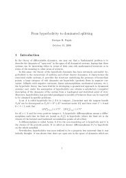
Figure 2.1: Two-fluid system configuration.
over h 2 is the undisturbed thickness of the lower layer outside the irregular bottom
region and it is comparable with the characteristic wavelength L, that characterizes
an intermediate depth regime. In the slowly varying bottom case we define
ε=L/l≪1; when a more rapidly varying bottom is of concern, the horizontal
length scale for bottom irregularities l is such that h 1 < l≪L. The coordinate
system is positioned at the undisturbed interface between layers. The displacement
of the interface is denoted byη(x, t) and we may assume that initially it has
compact support.
The corresponding Euler equations are
u ix + w iz = 0,
u it + u i u ix + w i u iz =− p ix
ρ i
,
w it + u i w ix + w i w iz =− p iz
ρ i
− g,
for i = 1, 2. Subscripts x, z and t stand for partial derivatives with respect to
spatial coordinates and time. The continuity condition at the interface z=η(x, t)
9

demands that
η t + u i η x = w i , p 1 = p 2 ,
namely, a kinematic condition for the material curve and no pressure jumps allowed.
At the top we impose a rigid lid condition,
w 1 (x, h 1 , t)=0,
commonly used in ocean and atmospheric models, while at the irregular impermeable
bottom
− h 2
l
h ′ ( x
l
)
u 2 + w 2 = 0.
Introducing the dimensionless dispersion parameterβ= ( )
h 1 2,
L it follows from
the shallowness of the upper layer that
O (√ β ) = O
( )
h1
≪ 1.
L
From the continuity equation for i=1we have,
w 1
u 1
= O
( )
h1
= O (√ β ) .
L
Let U 0 = √ gh 1 be the characteristic shallow layer speed. According to these
scalings, physical variables involved in the upper layer equations are non-dimen-
10

sionalized as follows:
x=L ˜x, z=h 1˜z, t= L U 0
˜t, η=h 1 ˜η,
u 1 = U 0 ũ 1 , w 1 = √ βU 0 ˜w 1 , p 1 = (ρ 1 U 2 0 ) ˜p 1.
In a weakly nonlinear theory,ηis usually scaled by a small parameter. Note that
here we have an O(1) scaling. This will lead to a strongly nonlinear model.
2.1 Reducing the upper layer dynamics to the interface
The dimensionless equations for the upper layer (the tilde has been removed) are:
u 1x + w 1z = 0,
u 1t + u 1 u 1x + w 1 u 1z =−p 1 x,
β ( w 1t + u 1 w 1x + w 1 w 1z
) =−p1 z− 1. (2.1)
The boundary conditions are
η t + u 1 η x = w 1 and p 1 = p 2 at z=η(x, t), (2.2)
w 1 (x, 1, t)=0.
Focusing on the upper shallow region, consider the following definition: for any
11

function f (x, z, t), let its associated mean-layer quantity f be
f (x, t)= 1 ∫ 1
f (x, z, t) dz.
1−η
η
By averaging we will reduce the 2D Euler equations to a 1D system.
Letη 1 = 1−η. From the horizontal momentum equation we have
η 1 u 1t +η 1 u 1 u 1x +η 1 w 1 u 1z =−η 1 p 1 x. (2.3)
We need to express each of these mean-layer quantities in terms of u 1 andη.
The difficulty at this stage is breaking up the mean of square, and other general
quadratic terms, into individually averaged terms. To begin with, note that
∫ 1
(η 1 u 1 ) t = u 1t dz−η t u 1 (x,η, t),
η
=η 1 u 1t −η t u 1 ,
where u 1 is evaluated at the interface (x, z, t)=(x,η(x, t), t). So,
η 1 u 1t = (η 1 u 1 ) t +η t u 1 . (2.4)
Similarly
η 1 u 1x = u 1 η x + (η 1 u 1 ) x , (2.5)
and
2η 1 u 1 u 1x =η x u 2 1 + (η 1 u 2 1
)
x
. (2.6)
12

Therefore at z=η(x, t),
η 1 (u 1t + u 1 u 1x )=(η 1 u 1 ) t + u 1 η t + 1 2 η xu 2 1 + 1 2
( )
η 1 u 2 1
.
x
From the kinematic condition Eq. (2.2)
u 1 η t + 1 2 η xu 2 1 = u 1w 1 − 1 2 η xu 2 1 ,
and by substitution,
η 1 (u 1t + u 1 u 1x )=(η 1 u 1 ) t + u 1 w 1 − 1 2 η xu 2 1 + 1 2
( )
η 1 u 2 1
. (2.7)
x
On the other hand, integration by parts and incompressibility give
∫ 1 ∫ 1
η 1 w 1 u 1z =−w 1 u 1 − w 1z u 1 dz=−w 1 u 1 + u 1x u 1 dz.
η
η
From Eq. (2.6),
η 1 w 1 u 1z =−w 1 u 1 + 1 2 η xu 2 1 + 1 2
( )
η 1 u 2 1
. (2.8)
x
Substituting Eqs. (2.7) and (2.8) in Eq. (2.3), the following mean-layer equation
is derived
(η 1 u 1 ) t +
( )
η 1 u 2 1
=−η 1 p 1 x. (2.9)
x
The incompressibility condition gives w 1 =η 1 u 1x at z=η(x, t). This, together
with Eq. (2.5) shows that
w 1 = u 1 η x + (η 1 u 1 ) x .
13

Substitution of w 1 into Eq. (2.2) leads toη t + u 1 η x = u 1 η x + (η 1 u 1 ) x and
−η 1 t= (η 1 u 1 ) x . (2.10)
As pointed in [8], the system of Eqs. (2.9)–(2.10) was already considered in
[31, 5] for surface waves. In reducing (averaging) the 2D Euler equations to this
1D system no approximations have been made up to this point. Nevertheless, the
quantities u 1· u 1 and p 1 x prevent the closure of the system of Eqs. (2.9)–(2.10).
These quantities will be expressed in terms ofηand u 1 up to a certain order in
the dispersion parameterβ. Note that until now, we still have not used the vertical
momentum equation and the continuity of pressure boundary condition. We start
by approximating p 1 x and then proceed to do the same for u 1· u 1 .
The vertical momentum equation over a shallow layer suggests the following
asymptotic expansion in powers ofβ
f (x, z, t)= f (0) +β f (1) + O(β 2 )
for any of the functions u 1 , w 1 , p 1 . In fact, from Eq. (2.1), p 1 z
=−1+O(β).
Integrating fromηto z we have that
p 1 (x, z, t)− p 1 (x,η, t)=−(z−η)+O(β),
and the pressure continuity across the interface gives
p 1 (x, z, t)= p 2 (x,η, t)−(z−η)+O(β).
14

The pressure p 2 (x,η, t) should be non-dimensionalized in the same fashion as p 1 ,
that is,
p 2 =ρ 1 U 2 0 ˜p 2.
Define P(x, t)= p 2
( x,η(x, t), t
) . Then
p 1 = P(x, t)−(z−η)+O(β),
which immediately yields
p 1 x=P x (x, t)+η x + O(β).
By averaging we get
p 1 x= 1 ∫1
η 1
η
P x (x, t) dz+η x + O(β),
= P x (x, t)+η x + O(β),
(
( ) ) = p 2 x,η(x, t), t x + O(β). (2.11)
x+η
An approximation for P x will be obtained later from the Euler equations for
the lower fluid layer. We now approximate the mean squared horizontal velocity
in terms of u 1 andη.
In order to express u 1· u 1 as a function of u 1 andη, it should be pointed out
that the irrotational condition in non-dimensional variables is
U 0
h 1
u 1z = √ β U 0
L w 1x,
15

i. e. u 1z =βw 1x . Hence ( )
u (0)
1
= 0 and as expected for shallow water flows u(0)
z 1
is
independent from z:
u (0)
1
= u (0) (x, t). (2.12)
1
We now correct this first order approximation. By using
u 1 = u (0)
1
+βu (1)
1
+ O(β 2 ) (2.13)
and Eq. (2.12) it is straightforward that
∫ 1
η
∫1
u 2 1 dz=
u 2 1 = u(0)
2
1 + 2βu
(1)
1 u(0) 1
+ O(β 2 ),
η
u (0)
1
∫1
2
dz+2β
η
u (1)
1 u(0) 1
dz+O(β 2 ),
and
η 1 u 1· u 1 = u (0) 2
1 (1−η)+2η1 βu (0)
1 u(1) 1
+ O(β 2 ),
so that
Also from Eq. (2.13),
u 1· u 1 = u (0)
1
· u (0)
1
+ 2βu (0)
1 u(1) 1
+ O(β 2 ). (2.14)
∫1
1
u 1 dz=u (0)
1
+βu (1)
1
+ O(β 2 ),
η 1
η
u 1 = u (0)
1
+βu (1)
1
+ O(β 2 ),
u 1· u 1 = u (0)
1
· u (0)
1
+ 2βu (0)
1 u(1) 1
+ O(β 2 ). (2.15)
16

Thus Eqs. (2.14) and (2.15) lead to our desired approximation, namely that
η 1 u 1· u 1 =η 1 u 1· u 1 + O(β 2 ). (2.16)
Using Eq. (2.16), the nonlinear interfacial system (2.9) becomes
η 1 tu 1 +η 1 u 1t + ( η 1 u 1· u 1 + O(β 2 ) ) x =−η 1p 1 x,
η 1 tu 1 +η 1 u 1t + u 1 (η 1 u 1 ) x +η 1 u 1· u 1x =−η 1 p 1 x+ O(β 2 ).
From Eq. (2.10) one obtains that
η 1 u 1t +η 1 u 1· u 1x =−η 1 p 1 x+ O(β 2 ). (2.17)
After substitution of Eq. (2.11), the following set of approximate equations for the
upper layer was derived from Eqs. (2.9), (2.10):
η 1 t+ (η 1 u 1 ) x = 0,
u 1t + u 1· u 1x =−η x −
(
p 2
( x,η(x, t), t
) ) x+ O(β),
or equivalently,
⎧
⎪⎨
−η t + ( (1−η)u 1
)x = 0,
⎪⎩ u 1t + u 1· u 1x =−η x −
(
p 2
( x,η(x, t), t
) ) x+ O(β).
(2.18)
We have almost closed our system of PDEs. Now we need to get an expression
for p 2 in order to close the system and also to establish a connection with the lower
17

fluid layer.
2.2 Connecting the upper and lower layers
The coupling of the upper and lower layers is done through the pressure term. To
(
( ) ) get an approximation for P x (x, t)= p 2 x,η(x, t), t from the Euler equations for
x
the lower fluid layer, notice that out of the shallow water approximation
h 2
L = O(1),
so that the following scaling relation
w 2
u 2
= O
( )
h2
= O(1)
L
follows from the continuity equation. At the interface, from the kinematic conditions
and the relations above, we have that
w 2
u 1
= O (√ β ) ,
u 2
u 1
= O (√ β ) ,
at z=η. Following these scalings introduce the dimensionless variables for the
lower region (with a tilde)
x=L ˜x, z=L˜z, t= L U 0
˜t, η=h 1 ˜η,
p 2 = (ρ 1 U 2 0 ) ˜p 2, u 2 = √ βU 0 ũ 2 , w 2 = √ βU 0 ˜w 2 .
18

This naturally suggests that we introduce the velocity potencialφ= √ βU 0 L ˜φ.
Note that the definition for ˜z is different from the one for the upper region, since
it involves the characteristic wavelength L instead of the vertical scale h 2 . This is
consistent since both scales are of the same order.
In these dimensionless variables, the Bernoulli law for the interface reads
√
βφt + β ( φ
2
2 x +φ 2 ρ 1
z) +η+ P=C(t),
ρ 2
where the tilde has been ignored.C(t) is an arbitrary function of time. Then, up
to orderβ, the pressure derivative P x is
P x =− ρ (
2 ηx + √ β ( φ t (x, √ βη, t) ) )
+ O(β), (2.19)
ρ 1
x
whereφsatisfies the Neumann problem with a free upper surface boundary condition,
given as
⎧
φ xx +φ zz = 0, on− h 2
L + h 2h(Lx/l)
L
≤ z≤ √ βη(x, t),
⎪⎨
φ z =η t + √ βη x φ x ,
at z= √ βη(x, t),
(2.20)
⎪⎩
− h 2
l h′ (Lx/l)φ x +φ z = 0, at z=− h 2
L + h 2h(Lx/l)
.
L
19

Furthermore,
[√ ( √ )]
βφt x, βη, t =√ ( √ ) ( √ )
βφ tx x, βη, t +βφtz x, βη, t ηx ,
x
= √ ( √ )
βφ tx x, βη, t + O(β),
= √ βφ tx (x, 0, t)+O(β),
where a Taylor expansion about z=0 was performed.
Therefore,
P x =− ρ 2
ρ 1
(
ηx + √ βφ tx (x, 0, t) ) + O(β). (2.21)
As in the flat bottom case [8], from Eq. (2.21) it is clear that it is sufficient to
find the horizontal velocityφ x at z=0 in order to obtain P x at the interface. Due
to the presence of the small parameter √ β in problem (2.20),φ x (x, 0, t) can be
approximated by the horizontal velocity at z=0 that comes from the linearized
problem around z=0,
⎧
φ xx +φ zz = 0, on− h 2
L + h 2h(Lx/l)
L
≤ z≤0,
⎪⎨
φ z =η t ,
at z=0,
(2.22)
⎪⎩
− h 2
l h′ (Lx/l)φ x +φ z = 0, at z=− h 2
L + h 2h(Lx/l)
.
L
In this systematic reduction we use Taylor expansion to ensure that
φ z (x, 0, t)=φ z
(
x,
√
βη, t
)
+ O
(√
β
)
,
=η t + √ βη x φ x + O (√ β ) ,
20

z=0
h 2
L
z=− h 2
L + h 2
L h(Lx/l)
ζ= 0
h 2
L
ζ=− h 2
L
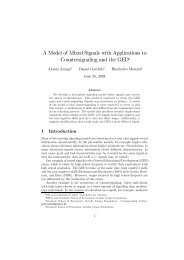
Figure 2.2: Conformal mapping, (x, z)= ( x(ξ,ζ), z(ξ,ζ) ) .
and therefore,
φ z (x, 0, t)=η t + O (√ β ) .
To find the horizontal velocityφ x (x, 0, t) in problem (2.22), a conformal mapping
between the flat stripζ∈ [ − h 2
L , 0] and the lower layer at rest is performed.
See Fig. 2.2.
21

The problem in conformal coordinates is
⎧
φ ξξ +φ ζζ = 0, on− h 2
L
≤ζ≤ 0,
⎪⎨
⎪⎩
( )
φ ζ (ξ, 0, t)= M(ξ)η t x(ξ, 0), t , atζ= 0,
(2.23)
φ ζ = 0, atζ=− h 2
L ,
where the previous Neumann condition at the top is now modified by M(ξ)=
z ζ (ξ, 0) which is the nonzero element of the Jacobian of the conformal mapping at
the unperturbed interface. As shown in [24], its exact expression is:
M(ξ 0 )=1− π 4
L
∫∞
h 2
−∞
h ( Lx(ξ,−h 2 /L)/l )
cosh 2( πL
2h 2
(ξ−ξ 0 ) ) dξ.
Moreover, the Jacobian along the unperturbed interface is an analytic function.
Hence a highly complex boundary profile has been converted into a smooth
variable coefficient in the equations.
To obtain the Neumann condition at the unperturbed interface in problem
(2.23), consider
φ ζ =φ x x ζ +φ z z ζ
evaluated at z=0 (equivalentlyζ= 0):
φ ζ (ξ, 0, t)=φ x (x, 0, t) x ζ (ξ, 0)+φ z (x, 0, t) z ζ (ξ, 0).
The Cauchy-Riemann relations and the fact that z(ξ, 0)=0 and z ξ (ξ, 0)=0 imply
22

that x ζ (ξ, 0)=0, which leads to the Neumann condition in problem (2.23).
Since a conformal mapping was used in the coordinate transformation and
z ξ (ξ, 0)=0, it is guaranteed that z ζ (ξ, 0)=x ξ (ξ, 0) is different from zero. From
φ ξ (ξ, 0, t)=φ x (x, 0, t) x ξ (ξ, 0), the velocityφ x (x, 0, t) is recovered as
φ x (x, 0, t)= φ ξ(ξ, 0, t)
.
M(ξ)
The bottom Neumann condition is trivial in these new coordinates.
Notice that the terrain-following velocity componentφ ξ (ξ, 0, t) is a tangential
derivative on the boundary for problem (2.23). Hence it can be obtained as the
Hilbert transform on the strip (see [15]) applied to the Neumann data. Namely
φ ξ (ξ, 0, t)=T [ φ ζ (˜ξ, 0, t) ] (ξ),
and substituting the Neumann data from problem (2.23),
φ ξ (ξ, 0, t)=T [ M(˜ξ)η t
( x(˜ξ, 0), t ) ]
(ξ),
where
T [ f ](ξ)= 1 2h
π
)
f (˜ξ) coth(
2h (˜ξ−ξ)
d ˜ξ (2.24)
is the Hilbert transform on the strip of height h. In this case, h=h 2 /L. The
singular integral must be interpreted as a Cauchy principal value. The effect of
the two-dimensional undisturbed layer below the interface is being collapsed onto
a one-dimensional singular integral without any approximation. The results above
are used in (2.21) by noting thatφ tx is obtained after taking the time derivative of
23

problem (2.22). Therefore,
P x =− ρ (
2
η x + √ 1
β
ρ 1 M(ξ) T[ (
M(˜ξ)η tt x(˜ξ, 0), t ) ]
)
(ξ) + O(β). (2.25)
Now,φ x (x, 0, t) is a tangential derivative on the flat upper boundary for problem
(2.22), whose domain is a corrugated strip. Hence, it is also expressed as a
Hilbert transform acting on Neumann data. Since
φ x (x, 0, t)=
L
2h 2 M ( ξ(x, 0) )
(
M(˜ξ)η t x(˜ξ, 0), t ) ( πL
coth
(˜ξ−ξ(x, 0) )) d ˜ξ,
2h 2
a Hilbert-like transform on the corrugated strip has been identified as:
T c [ f ](x)=
L
2h 2 M ( ξ(x, 0) )
M(˜ξ) f ( x(˜ξ, 0) ) ( πL
coth
(˜ξ−ξ(x, 0) )) d ˜ξ,
2h 2
which is not a convolution operator, unlike Eq. (2.24).
Finally, substituting the expression for P x obtained in Eq. (2.25) in the upper
layer averaged equations (2.18) gives
⎧
η t − [ (1−η)u 1
]x
(
= 0,
⎪⎨ u 1t + u 1 u 1x + 1− ρ )
2
η x =
ρ 1
√
L ρ 2 1
⎪⎩ β
2h 2 ρ 1 M ( ξ(x, 0) ) (
M(˜ξ)η tt x(˜ξ, 0), t ) ( πL
coth
(˜ξ−ξ(x, 0) )) d ˜ξ+ O(β).
2h 2
In a compact notation this becomes
⎧
η
⎪⎨ t − [ (1−η)u 1
]x
(
= 0,
⎪⎩ u 1t + u 1 u 1x + 1− ρ )
2
η x = √ β ρ 2 1
ρ 1 ρ 1 M(ξ) T[ ( )]
M(·)η tt x(·, 0), t (ξ)+O(β),
24

where the dot indicates the variable on which the operatorT is applied.
It remains to make a few manipulations with this set of equations: eliminate
the second order derivative in time and write all spatial derivatives in the
ξ-variable.
Note that the first equation is exact. According to itη tt = ( (1−η)u 1
)xt
so
only the first time derivative of u 1 needs to enter the right-hand side of the second
equation.
In conclusion, the reduced one-dimensional internal wave model is:
⎧
η
⎪⎨ t − [ (1−η)u 1
]x
(
= 0,
⎪⎩ u 1t + u 1 u 1x + 1− ρ )
2
η x = √ β ρ 2 1
ρ 1 ρ 1 M(ξ) T[ M(·) ( ) )]
(1−η)u 1 xt(
x(·, 0), t .
(2.26)
The transform in the forcing term is in curvilinear coordinates. For practical
purposes both sides must be in the same coordinate system, which is readily adjusted
via the conformal mapping: every x-derivative is equal to aξ-derivative
divided by the Jacobian M(ξ). Therefore, system (2.26) in the terrain-following
coordinates reads
⎧
η t − 1 [ ] (1−η)u1
⎪⎨ M(ξ)
⎪⎩
ξ = 0,
u 1t + 1
M(ξ) u 1 u 1ξ + 1
M(ξ)
(
1− ρ )
2
η ξ = √ β ρ 2 1
ρ 1 ρ 1 M(ξ) T[ ( ) ] (2.27)
(1−η)u1
ξt .
This is a Boussinesq-type system with variable (time independent) coefficients
depending on M(ξ) for the perturbation of the interfaceηand the mean-layer
horizontal upper velocity u 1 . We will show that this is a dispersive model, where
the dispersion term comes in through the Hilbert transform. Since no smallness
25

assumption was made on the wave amplitude up to now, the model derived is
strongly nonlinear. It involves a Hilbert transform on the strip characterizing the
presence of harmonic functions (hence the potential flow) below the interface.
System (2.27) is a reduction of the original Euler equations constituted by
a pair of 2D-systems of PDEs to a single 1D-system of PDEs at the interface.
Instead of the integration of the Euler equations in the presence of a free interface,
a single 1D-system of PDEs is to be solved. Efficient computational methods can
be produced for this accurate reduced model which governs, to leading order, a
complex two-dimensional problem.
Remarks:
1. If the bottom is flat, M(ξ)=1 and the same system derived in [8] is recovered,
which is a nice consistency check.
2. When the lower depth tends to infinity (h 2 →∞) the limit for this model
is the same one obtained in [8] because the bottom is not seen anymore
(M(ξ)→1 and x(˜ξ, 0)→ ˜ξ). Therefore
φ xt (x, 0, t)→ 1 π
( ) ( )
(1−η)u1
xt ˜x, t
˜x− x
[ ((1−η)u1 )
]
d ˜x=H
xt
(x),
whereH is the usual Hilbert transform defined as
H[ f ](x)= 1 π
f ( ˜x)
˜x− x d ˜x.
In this (shallow upper layer) infinite lower layer regime, system (2.26) be-
26

comes
⎧
η
⎪⎨ t − [ (1−η)u 1
]x = 0,
⎪⎩ u 1t + u 1 u 1x +
(
1− ρ )
2
η x = √ β ρ 2
H
ρ 1 ρ 1
[ ((1−η)u1 )
]
xt.
(2.28)
3. The Fourier Transform (FT) of a Hilbert transform is easily computed. We
now make a comment regarding the use of FTs in numerical schemes. The
operatorsT [ f ] andH[ f ] have Fourier transforms
) kh2
̂T [ f ]=i coth(
f, ˆ
L
Ĥ[ f ]=i sgn(k) ˆ f,
where the operator symbol multiplies the transform of f , which is ˆ f . Therefore
in Eqs. (2.27) and (2.28) a pseudospectral scheme would apply a DFT
to the terms inside the square brackets. FFTs are only aplicable directly
when M(ξ)=1 and the waves are weakly nonlinear.
2.3 Dispersion relation for the linearized model
Consider the flat bottom case in system (2.26), that is, M≡ 1:
⎧
η
⎪⎨ t − [ (1−η)u 1
]x
(
= 0,
⎪⎩ u 1t + u 1 u 1x + 1− ρ )
2
η x = ρ √ [
2 ((1−η)u1 )
]
βT
xt
+ O(β).
ρ 1 ρ 1
27

Its linearization around the undisturbed stateη=0, u 1 = 0 gives:
⎧
η
⎪⎨ t − u 1x = 0,
(
⎪⎩ u 1t + 1− ρ )
2
η x = ρ √
2 [ ] βT u1xt .
ρ 1 ρ 1
By differentiating once in t,ηcan be eliminated from the second equation:
u 1tt +
(
1− ρ )
2
u 1xx = ρ √
2 [ ] βT u1xtt .
ρ 1 ρ 1
Let u 1 = Ae i(kx−ωt) and substituting above,
e i(kx−ωt) (−ω 2 −
(
1− ρ ) )
2
k 2 = ρ √
2 β kω 2 e −iωt T [ −ie ikx] .
ρ 1 ρ 1
SinceT [e ikx ]=i coth ( )
kh 2
L e ikx ,
ω 2 =
(
ρ2
ρ 1
− 1 ) k 2
1+ ρ √ (
2
ρ 1
βk coth
kh2
L
), (2.29)
which is the correct approximation for the full dispersion relation
ω 2 =
(
ρ2
ρ 1
− 1 ) k 2
kh 1
coth( )
kh 1
L L +
ρ 2
√ (
ρ 1
βk coth
kh2
)
L
when kh 1 is near zero. A nonvanishing value of the parameterβin the dispersion
relation makes the phase velocity a function of the wave number k. Observe that
ω 2
k 2
→ 0 as k→∞, so bounded phase velocities are obtained as k becomes large.
This is a good property for numerical schemes.
In the limit h 2 →∞ the operatorT becomesH. SinceH[e ikx ]=i sgn(k)e ikx ,
28

the dispersion relation for system (2.28) is
ω 2 =
(
ρ2
ρ 1
− 1 ) k 2
1+ ρ √
2
ρ 1
β|k|
and ω2
k 2
→ 0 as k→∞.
2.4 Unidirectional wave regime
For weakly nonlinear unidirectional waves and slowly varying topography, our
model reduces to a single ILW equation with variable coefficients.
Consider again system (2.26), except for the Jacobian of the conformal mapping
which now is
M(ξ 0 )=1− π 4
L
∫∞
h 2
−∞
h ( εx(ξ,−h 2 /L) )
cosh 2( πL
2h 2
(ξ−ξ 0 ) ) dξ,
since we assume a slowly varying bottom topography described in non-dimensional
coordinates as z=− h 2
+ h 2
L L
h(εx), withε≪1. The restriction to a slowly
varying topography is consistent with the objective of the present Section, which
is to find equations to model the unidirectional wave propagation. Hence there will
be no reflection nor any backward evolution opposite to the propagation direction.
To study the weakly nonlinear regime, we introduce the typical amplitude a for
the perturbation of the interface and introduce the nonlinearity parameterα= a h 1
of
order O ( √ β
)
. As usual in a weakly nonlinear theory we setη=αη ∗ . With this, the
original dimensional perturbationηis non-dimensionalized asη=αh 1 η ∗ = aη ∗ .
We also state that u 1 =αc 0 u 1 ∗ , t= t∗
c 0
where c 2 0 =( ρ 2
ρ 1
− 1 ) . Depending on the root
29

c 0 chosen, there will be a right- or left-travelling wave.
Then, dropping the asterisks, Eq. (2.26) becomes
⎧
η ⎪⎨ t − [ (1−αη)u 1
]x = 0,
⎪⎩ u 1t +αu 1 u 1x −η x = √ β ρ 2 1
ρ 1 M(ξ) T[ M(˜ξ) [ ] ] (2.30)
(1−αη)u 1 xt + O(β).
Note that
η t = u 1x + O(α); η x = u 1t + O ( α, √ β ) . (2.31)
As in [8], we look for a solution, up to a first order correction inαand √ β, in
the form
η=A 1 u 1 +αA 2 u 1 2 + √ β A 3
1
M(ξ) T[ M(˜ξ)u 1t
]
. (2.32)
Substituting in the system of Eqs. (2.30) up to orderα, √ β, two equations for
u 1 are obtained:
0=A 1 u 1t + 2αA 2 u 1 u 1t + 2αA 1 u 1 u 1x − u 1x + √ β A 3
1
M(ξ) T[ M(˜ξ)u 1tt
]
and
0=u 1t +αu 1 u 1x −
[
A 1 u 1x + 2α A 2 u 1 u 1x + √ β A 3
1
M(ξ) T[ M(˜ξ)u 1xt
] ] −
− √ β ρ 2
ρ 1
1
M(ξ) T[ M(˜ξ)u 1xt
]
+ O
(
α 2 ,β,α √ β ) .
For compatibility A 1 =±1 and to choose a right-going wave we take A 1 =−1.
Therefore
η x =−u 1x + O ( α, √ β ) , (2.33)
30

so u 1t =−u 1x + O ( α, √ β ) and u 1tt =−u 1xt + O ( α, √ β ) and the two equations are
consistent if A 1 =−1, A 2 =− 1 4 and A 3=− ρ 2
2ρ 1
. As a result, the evolution equation
for u 1 is
u 1t + 3 2 αu 1 u 1x + u 1x − ρ √
2 β 1
ρ 1 2 M(ξ) T[ ] (
M(˜ξ)u 1xt = O β,α 2 ,α √ β ) .
For the elevation of the interfaceηasimilar equation can be obtained through
asymptotic relations which permit (to leading order) to exchange derivatives inη
by derivatives in u 1 , as well as time derivatives for spatial derivatives. This is a
consequence of (2.32). To begin with, use that
u 1xt =−η xt + O ( α, √ β )
so
√ β
2
ρ 2 1
ρ 1 M(ξ) T[ ]
√ β
M(˜ξ)u 1xt =−
2
ρ 2
1
ρ 1 M(ξ) T[ ] (
M(˜ξ)η xt + O α 2 ,β,α √ β ) . (2.34)
In virtue of Eqs. (2.33) and (2.32)
3
2 αu 1 u 1x = 3 2 α( −η x + O ( α, √ β ))( −η+O ( α, √ β )) ,
= 3 2 αηη x+ O ( α 2 ,α √ β ) , (2.35)
31

and for similar reasons
η t +η x =− (u 1t + u 1x )− α 2 u 1(u 1t + u 1x )−
√ β
2
ρ 2 1
ρ 1 M(ξ) T[ M(˜ξ)(u 1tt + u 1xt ) ] ,
=− (u 1t + u 1x )+O ( α 2 ,α √ β,β ) . (2.36)
Substituting all these expressions in the evolution equation for u 1 we obtain
the evolution equation for the elevation of the interface,
η t +η x − 3 2 αηη x− ρ √
2 β 1
ρ 1 2 M(ξ) T[ ] (
M(˜ξ)η xt = O β,α 2 ,α √ β ) .
Finally, in curvilinear coordinates we have
η t + 1
M(ξ) η ξ− 3 2
α
M(ξ) ηη ξ− ρ √
2 β
ρ 1 2
1
M(ξ) T [η ξt]=0. (2.37)
This is an ILW equation with variable coefficients accounting for the slowly
varying bottom topography. Instead of the usual Hilbert transform on the halfspace,
a Hilbert transform on the strip appears. The dispersion relation for the flat
bottom case (M(ξ)=1) is
ω=
k
1+ ρ √
2 β
k coth( ). (2.38)
kh 2
ρ 1 2 L
The equation reduces to a regularized dispersive model in analogy with the Benjamin-
Bona-Mahony equation (BBM), [4].
Remarks:
1. The constant coefficient version of Eq. (2.37) differs from the ILW consid-
32

ered in [8], Eq. (4.33), page 23, in that the latter has a dispersion term with
spatial derivatives only, as in the KdV equation. Both constant coefficient
equations are equivalent up to the order considered since we can substituteη
ξt by−η ξξ in the dispersion term up to order O ( β,α √ β ) . There are
two advantages for our choice. First, for every change from a Cartesian
x-derivative to a curvilinearξ-derivative we need the presence of the metric
term M(ξ). Hence for the Camassa-Choi model with the second order
x-derivative we would end up with a variable coefficient within the nonlocal
operator. Second, the regularized dispersive operator (namely with an
xt-derivative) leads to the stable dispersion relation (2.38) regarding numerical
schemes. Short waves have bounded propagation speeds. This does not
happen with the ILW equation considered in [8], whose dispersion relation
is
ω=k− ρ √ ( )
2 β kh2
ρ 1 2 k2 coth .
L
2. One step remains to be explained in the substitution of Eq. (2.32) into the
second equation of system (2.30), namely why it is valid (for slowly varying
topography) that
( √ β
M(ξ) T[ ] )
M(˜ξ)u 1t =
x
√ β
M(ξ) T[ M(˜ξ)u 1tx
]
+ O(β). (2.39)
This approximation was not presented in [8] since the present work contains
for the first time the conformal mapping technique used for the lower
layer. The approximation (2.39) is justified through the construction of an
auxiliary PDE problem. See Appendix A for details.
33

3. For system (2.28) a similar unidirectional reduction can be obtained leading
to
η t +η x − 3 2 αηη x− ρ 2
ρ 1
√ β
2 H[η xt]=0,
which is a regularized Benjamin-Ono (BO) equation over an infinite bottom
layer.
Hence Eq. (2.37) is a generalization of the BO equation for intermediate
depth and the presence of a topography. This equation is valid only when
backscattering is negligible.
2.5 Solitary wave solutions
The ILW equation we referred to in Section 2.4 and derived in [8, 14, 17] is of the
form
η t +η ξ + c 1 ηη ξ + c 2 T [η ξξ ]=0 (2.40)
where c 1 =− 3 2 α and c 2= ρ 2
√ β
ρ 1 2
solitary wave solutions [14, 8]
. Eq. (2.40) admits a family in the parameterθof
η(x)=
a cos 2 θ
, x=ξ− ct, (2.41)
cos 2 θ+sinh 2 (x/λ)
where
a= 4c 2θ tanθ
h 2 c 1
, λ= h 2
θ , c=1− 2c 2
h 2
θ cot(2θ),
with 0≤θ≤π/2. Alternatively, we consider a Regularized Intermediate Long
Wave equation
η t +η ξ + c 1 ηη ξ − c 2 T [η ξt ]=0 (2.42)
34

to the same order of approximation. It also admits the solitary wave solution
Eq. (2.41) with
a= 4c 2
h 2 c 1
θ tanθ
1+ 2c 2
h 2
θ cot(2θ) , λ= h 2
θ , c= 1
1+ 2c 2
h 2
θ cot(2θ) .
In the numerical section we will present a few experiments with solitary waves
over a flat bottom. In the near future we intend to study solitary waves interacting
with highly varying topography and submarine structures.
35

Chapter 3
A higher-order reduced model
Since we want to study wave interaction with highly variable topographies and
submarine structures, we need to be able to account for higher order (vertical)
coupling terms between the two layers. Namely we want to investigate if these
higher order terms do indeed play a role in the dynamics. Hence in this chapter
we improve the model from the previous chapter regarding the pressure term by
allowing nonhydrostatic terms to come into play.
3.1 Higher-order upper layer equations
The purpose of this chapter is to improve the order of approximation of system
(2.27) by using higher precision approximations for the pressure term with
respect to the dispersion parameterβ. Instead of orderβ, we seek order O(β 3/2 ).
We start with the mean-layer equations (2.10) and (2.17) obtained in Section 2.1.
36

For convenience they are repeated here:
η 1 t+ (η 1 u 1 ) x = 0, (3.1)
u 1t + u 1· u 1x =−p 1 x+ O(β 2 ). (3.2)
term:
To approximate p 1 x with orderβ 3/2 we need to expand p 1 (x, z, t) with one more
so its vertical derivative is expanded as
p 1 (x, z, t)= p (0)
1
+βp (1)
1
+ O(β 2 ),
p 1 z(x, z, t)= p (0)
1 z +βp(1) 1 z + O(β2 ). (3.3)
Again, from the vertical momentum equation
p 1 z=−1−β(w 1t + u 1 w 1x + w 1 w 1z )
we have that
p (0)
1 z =−1.
This is the hydrostatic contribution to the pressure. We also have that
p (1)
1 z =−(w(0) 1 t + u(0) 1 w(0) 1 x + w(0) 1 w(0) 1 z ).
Even though the upper layer is shallow, through p 1 we can compute the leading
order nonhydrostatic correction.
Let D 1 =∂t+u (0)
1∂x be the leading order material derivative. We rewrite the
37

expression above as
Let us express the quantities w (0)
1 z
expanding the incompressibility equation to obtain
p (1)
1 z =−D 1w (0)
1
− w (0)
1 z w(0) 1 . (3.4)
and w(0)
1
in terms ofηand u 1 . We begin by
w (0)
1 z =−u(0) 1
(x, t). (3.5)
x
Integrating Eq. (3.5) fromηto z≤1 and taking into account the z-independence
expressed by Eq. (2.12) we have that
w (0)
1
(x, z, t)=−u(0)
1
(x, t)(z−η)+w(0) ∣
x 1 z=η(x,t)
.
Now, from the kinematic condition in Eq. (2.2), to leading order
w (0)
1
∣ z=η(x,t)
=η t + u (0)
1 η x
so
that is,
w (0)
1
(x, z, t)=−u(0)
1 (x, t)(z−η)+η x t+ u (0)
1 η x,
w (0)
1
(x, z, t)=−u(0)
1 (x, t)(z−η)+ D x 1η. (3.6)
Substituting Eqs. (3.6) and (3.5) in Eq. (3.4):
p (1)
1 z = (z−η) (
D 1 (u (0)
1 x )−u(0)
2
1 x
)
− D 2 1 (η).
38

Since
u 1 = u (0)
1
+ O(β), (3.7)
it is also valid that
p (1)
1 = (z−η)( )
2
D
z 1 (u 1x )−u 1 x − D
2
1 (η)+O(β).
Recall thatη 1 = 1−η and now define
G 1 (x, t)= 1 η 1
(D 2 1 η).
It can be shown 1 that
G 1 (x, t)=D 1 (u 1x )−u 1
2
x+ O(β).
Therefore,
p (1)
1 z = (z−η)G 1(x, t)−η 1 G 1 (x, t)+O(β)
1 Write the conservation of mass Eq. (2.10) in the form
(∂t+u 1 ∂x)η 1 +η 1 u 1x = 0,
which together with the approximation (3.7) leads to
D 1 η 1 +η 1 u 1x = O(β),
which is the same as D 1 η=η 1 u 1x + O(β). Apply D 1 to it,
Expanding the right-hand side above we have
D 2 1 η=D 1(η 1 u 1x )+O(β).
D 1 (η 1 u 1x )+O(β)=η 1 (u 1xt + u 1 u 1xx )+u 1x (η 1t + u 1 η 1x )+O(β),
=η 1 (u 1xt + u 1 u 1xx − u 1x u 1x )+O(β),
=η 1
(
D1 (u 1x )−u 1
2
x
)
+ O(β).
Then D 2 1 η=η ( )
2
1 D1 (u 1x )−u 1x + O(β) as desired.
39

and substituting in the asymptotic expansion Eq. (3.3) for p 1 z we have
p 1 z(x, z, t)=−1+β(z−1)G 1 (x, t)+O(β 2 ).
Integrating from z=η(x, t) to z≤1 we obtain
( )
(z−1)
2
p 1 (x, z, t)=P(x, t)−(z−η)+βG 1 (x, t) − (η−1)2 + O(β 2 ).
2 2
Differentiating once in x,
( ( ))
(z−1)
2
p 1 x=η x + P x (x, t)+β G 1 (x, t) − (η−1)2 + O(β 2 )
2 2
x
and taking means
p 1 x=η x + P x (x, t)− β ( ) 1
η 1 3 η3 1 G 1(x, t) + O(β 2 ).
x
Substituting in Eq. (3.2) we have
(
u 1t + u 1· u 1x =− η x + P x (x, t)− β ( ))
1
η 1 3 η3 1 G 1(x, t) + O(β 2 ). (3.8)
x
If the lower fluid layer is neglected and P is regarded as the external pressure
applied to the free surface, Eqs. (3.1) and (3.8) are the complete set of evolution
equations for one homogeneous layer derived by Su and Gardner in [27] and
independently by Green and Naghdi in [11].
40

3.2 Improved approximation for pressure at the interface
Now we want an approximation of order O(β 3 2 ) for Px (x, t)=
(
p 2
( x,η(x, t), t
) ) x
from the Euler equations for the lower fluid layer. This order of approximation
is sufficient to make the nonhydrostatic orderβterms explicit in the asymptotic
expansion. Again, the scale √ β comes from the lower layer reduction.
From the Bernoulli law for the lower layer:
P(x, t)=− ρ ( √βφt
2
+ β )∣ ∣∣∣∣z=
ρ 1 2 (φ2 x+φ 2 z)+η+ C(t) .
√ βη(x,t)
Using a Taylor expansion about z=0 we obtain that
P(x, t)=− ρ (
2
η+ √ β ( φ t |
ρ z=0 + √ ) β
βηφ tz | z=0 +
1 2
(
φ
2
x
∣ ∣∣z=0
+φ 2 z∣
∣ z=0
)
+ C(t)
)+O(β 3 2 ).
Since from Eq. (2.20) we have thatφ z =η t + √ βη x φ x =η t + O ( √ β
)
at z=
√ βη(x, t), it follows that
φ z | z=0 =φ z | z=
√ βη + O (√ β ) =η t + O (√ β )
and
φ tz | z=0 =φ tz | z=
√ βη + O (√ β ) =η tt + O (√ β ) .
Therefore
P(x, t)=− ρ 2
(η+ √ βφ t |
ρ z=0 +βηη tt + β ( ∣
φ
2 ∣∣z=0
) )
1 2 x +η 2 t + C(t) + O(β 2 3 )
41

and it is easy to take x-derivatives since all quantities are evaluated at z=0:
P x (x, t)=− ρ (
2
η x + √ (
βφ tx |
ρ z=0 +β ηη tt + 1
1 2 η2 t+ 1 ))
2 φ2 x∣ z=0
+ O(β 2 3 ).
Note from the previous chapter thatφ x | z=0 is already known up to order √ β,
namely that
φ x
( x(ξ, 0), 0, t
) =
1
M(ξ) T [
M(˜ξ)η t
( x(˜ξ, 0), t )] (ξ)+O (√ β ) (3.9)
which is all we need to approximate 1 2 φ2 x∣ z=0
.
We will obtainφ x | z=0 with order of approximationβvia the Hilbert transform
on the corrugated strip. Assuming that our potential problem for the lower deep
layer is defined in a region surrounding the physical domain containing the interface
at rest z=0, we restrict our potential problem to the unperturbed region.
There the potential problem satisfies a certain upper Neumann boundary condition
(φ z | z=0 ) to be determined up to orderβ. This order of approximation is sufficient
to obtain an x-derivative of orderβbecause we are solving a linear problem and
we have the Hilbert transform connecting these two derivatives. The calculation
is as follows.
To obtainφ z | z=0 a Taylor expansion is used as before:
x
φ z
(
x,
√
βη
)
=φz (x, 0)+ √ βηφ zz (x, 0)+O(β).
Since the boundary conditionφ z
(
x,
√ βη
)
is known we have
φ z (x, 0)=η t + √ βη x φ x (x, 0)− √ βηφ zz (x, 0)+O(β)
42

and due to the Laplace equation,
φ z (x, 0)=η t + √ βη x φ x (x, 0)+ √ βηφ xx (x, 0)+O(β)
which is the same as
φ z (x, 0)=η t + √ β ( ηφ x (x, 0) ) x + O(β).
Using Eq. (3.9) in the expression above,
φ z (x, 0)=η t + √ (
β η 1
=η t +
√ β
M(ξ)
)
M(ξ) T [M(˜ξ)η t ]
(
η 1
M(ξ) T [M(˜ξ)η t ]
x
+ O(β),
)
+ O(β).
Thus by means of the Hilbert transform on the corrugated strip,
ξ
φ x (x, 0)= 1
M(ξ) T[ M(˜ξ)φ z (x, 0) ] ,
= 1
⎛ √ β
M(ξ)
⎡⎢⎣ T M(˜ξ) ⎜⎝ η t+
M(˜ξ)
= 1
M(ξ) T ⎡⎢⎣ M(˜ξ)η t + √ β
(
η 1
)
M(˜ξ) T [M(ξ′ )η t ]
ξ
) ⎤
(
η 1
M(˜ξ) T [M(ξ′ )η t ]
ξ
⎞⎤
⎟⎠⎥⎦ + O(β),
⎥⎦ + O(β).
It is easy to take a time-derivative of this expression since the coefficient M is
independent of t:
φ tx (x, 0)= 1
M(ξ)
⎡⎢⎣ T M(˜ξ)η t + √ (
β η 1 )
M(˜ξ) T [M(ξ′ )η t ]
ξ
⎤
⎥⎦ + O(β),
t
43

which together with
η tt = ( (1−η)u 1
)
xt =( (1−η)u 1
)ξt /M(ξ)
leads to
√
√ β
βφtx | z=0 =
M(ξ) T[ ( ) ]
[
β
(1−η)u1
ξt +
M(ξ) T η
M(˜ξ) T[ ( )] ]
(1−η)u1
ξ
+ O(β 3 2 ),
ξt
and as we saw
layer is
β( ∣
φ
2 ∣∣z=0
)
2
=β x x 2
=
=
⎛{ 1
⎜⎝
β
2M(ξ)
β
2M(ξ)
M(ξ) T[ ] } 2 ⎞
M(˜ξ)η t + O(β 2 ⎟⎠x
3 ),
⎛{ 1
⎜⎝
M(ξ) T[ ] } 2 ⎞
M(˜ξ)η t + O(β ⎟⎠ξ
3 2 ),
⎛{ 1
⎜⎝
M(ξ) T[ ( ) (1−η)u1 ξ] } 2 ⎞ ⎟⎠ + O(β 3 2 ).
ξ
Summarizing, the higher order pressure term connecting the top and lower
√ β
M(ξ) T[ ( ) (1−η)u1
ξt]
+
+ β [
M(ξ) T η
M(ξ) T[ ( )] ]
(1−η)u1
ξ
+
ξt
⎛{ β 1
+ ⎜⎝
2M(ξ) M(ξ) T[ ( ) (1−η)u1 ξ] } 2 ⎞ ⎟⎠ +
ξ
(
ηη tt + 1 2 η2 t)⎞⎟⎠ + O(β 3 2 ).
P x (x, t)=− ρ 2
ρ 1
⎛⎜⎝ η x+
+ β
M(ξ)
This order of approximation is compatible with the nonhydrostatic corrections
44

added to the upper shallow water layer model since it makes the orderβterms
explicit.
Notice that composition of the Hilbert operatorT arises in this case. A similar
situation also occurred in the fully dispersive Boussinesq model obtained by
Matsuno in [19] and Artiles and Nachbin in [1] for surface gravity waves.
The above pressure term is substituted into the system of Eqs. (3.1) and (3.8)
in curvilinear coordinates, that is,
⎧
⎪⎨
⎪⎩
η t = 1 ( ) (1−η)u1
ξ
M(ξ)
,
u 1t + 1
M(ξ) u 1 u 1ξ =− 1
M(ξ) η ξ+
β 1
(1−η) 3M(ξ)
( (1−η) 3 G 1
)
ξ − P x+ O(β 2 )
where
G 1 (ξ, t)= 1
M(ξ) u 1ξt+ u ( )
1 1
M(ξ) M(ξ) u 1ξ
ξ
−
1
M(ξ) 2 u 1ξu 1ξ .
As a result, the strongly nonlinear model of orderβ 3 2
is:
⎧
⎪⎨
⎪⎩
η t = 1 ( ) (1−η)u1
ξ
M(ξ)
,
u 1t + 1
M(ξ) u 1 u 1ξ + 1 (
1− ρ )
2
η ξ = ρ √
2 β
M(ξ) ρ 1 ρ 1 M(ξ) T[ ]
(1−η)u 1 ξt +
+ β ⎛
1 ( )
(1−η) 3 G 1
1−η 3M(ξ)
+ρ 2 β η ( (1−η)u 1
)ξt
⎜⎝ + 1 ⎞
) 2 (1−η)u1
ξ ξ⎟⎠
+
ρ 1 M(ξ) M(ξ) 2(
ξ
+ β [ ]
ρ 2 η
T
M(ξ) ρ 1 M(ξ) T[ ]
(1−η)u 1 ξ
+
ξt
{
β ρ 2 1
+
⎛⎜⎝
2M(ξ) ρ 1 M(ξ) T[ ( ) (1−η)u1 ξ] } 2 ⎞ ⎟⎠ + O(β 3 2 ),
ξ
45

For the weakly nonlinear model of orderβ 3 2 introduceη ∗ , u ∗ 1 such that
η=αη ∗ , u 1 =αu 1 ∗ ,
withα=O ( √ β
)
, a typical scaling used for solitary waves. After dropping the
asterisks we have
⎧
⎪⎨
⎪⎩
η t = 1 [ ] (1−αη)u1
ξ
M(ξ)
,
(
1− ρ )
2
η ξ = ρ 2
ρ 1 ρ 1
u 1t + α
M(ξ) u 1 u 1ξ + 1
M(ξ)
( )
β 1
+
3M(ξ) M(ξ) u 1ξt + O(β 2 3 ).
ξ
√ β
M(ξ) T[ (1−αη)u 1
]
ξt +
The higher-order weakly nonlinear model has exactly the same form as the
lower-order strongly nonlinear model when the last term, namely,
( )
β 1
3M(ξ) M(ξ) u 1ξt
of the weakly nonlinear model is neglected. This implies that the weakly nonlinear
higher-order model should serve as a good model for moderate amplitude internal
waves in a deep water configuration. Furthermore, when the additional term
from the upper layer is included, the linear dispersion relation for the higher-order
weakly nonlinear model becomes the closest to the exact linear dispersion relation
when compared to lower-order models, as will be shown in the next Section. In
other words, the weakly nonlinear higher-order model might have a large domain
of validity so that the model can be used for a moderate (although still large) ra-
ξ
46

tio of h 2 /h 1 , where the effects of bottom topography are more pronounced. This
might be a justification for using a higher-order weakly nonlinear model and will
be thoroughly explored in the near future.
3.3 Dispersion relation for the higher-order model.
Comparison with the previous model
To obtain the dispersion relation for the improved model, consider its linearization
around the undisturbed state so that
⎧
⎪⎨
⎪⎩
η t = u 1ξ ,
u 1t +
(
1− ρ )
2
η ξ = ρ √
2 βT[u1 ] ξt + β ρ 1 ρ 1 3 u 1ξξt,
in the presence of a flat bottom.
Taking derivatives once in t,ηcan be eliminated from the second equation,
u 1tt +
(
1− ρ )
2
u 1ξξ − ρ √
2 βT[u1 ] ξtt − β ρ 1 ρ 1 3 u 1ξξtt= 0.
Let u 1 = Ae i(kx−ωt) . Substituting above and using again thatT [e ikx ]=i coth ( )
kh 2
L e
ikx
we get
(
ω 2 1+ β 3 k2 + ρ ( )) ( )
√
2 kh2 ρ2
β k coth = − 1 k 2 ,
ρ 1 L ρ 1
that is,
ω 2 =
(
ρ2
ρ 1
− 1 ) k 2
1+ β 3 k2 + ρ √ (
2
ρ 1
β k coth
kh2
L
). (3.10)
47

Again, ω2
k 2
large.
→ 0 as k→∞, so bounded phase velocities are obtained as k becomes
Now, let us make a comparison between the different dispersion relations obtained
throughout this work. Initially, we have the dimensional full dispersion
relation
ω 2 f=
g(ρ 2 −ρ 1 )k 2
ρ 1 k coth(kh 1 )+ρ 2 k coth(kh 2 )
(3.11)
that comes from the linearized Euler equations around the undisturbed state, see
for example [18]. To compare it with the dimensionless dispersion relations (2.29)
and (3.10) it must be taken into account that because of the non-dimensionalization,
k= k L , ω= U 0
L ω.
Therefore, (2.29) in dimensional form becomes
ω 2 g(ρ 2 −ρ 1 )k 2
r= ρ 1
h 1
+ρ 2 k coth(kh 2 ) . (3.12)
As it has been stated, the reduced model (2.27) captures the dispersion relation for
the shallow water (long waves) regime in the upper layer since
ρ 1 k coth(kh 1 )→ ρ 1
h 1
,
as kh 1 → 0.
On the other side, the relation (3.10) in dimensional form is
ω 2 h = g(ρ 2 −ρ 1 )k 2
ρ 1
h 1
+ 1h 3 1ρ 1 k 2 +ρ 2 k coth(kh 2 ) .
48

Notice that both approaches are fully dispersive regarding the bottom layer, since
the second coth is completely retained. For the shallow water upper layer regime
(kh 1 near zero) we obtain again the correct approximation of the full dispersion
relation, but here the termρ 1 k coth(kh 1 ) in the denominator is expanded with one
more term, namely
ρ 1
kh 1 coth(kh 1 )= ρ (
1
1+ (kh 1) 2
+ O ( (kh 1 ) 4)) ,
h 1 h 1 3
and consequently
ω 2 f=ω 2 h + O( (kh 1 ) 4) ,
while
ω 2 f=ω 2 r+ O ( (kh 1 ) 2) .
This means that the linear dispersion relation from the higher-order nonlinear
modelω 2 h is closer to the full (exact) linear dispersion relationω2 f
than the linear
dispersion relation from the lower-order modelω 2 r is. See Fig. 3.1 and a detail
in Fig. 3.2 where the corresponding phase velocities are depicted.
The inclusion of the higher order pressure term has improved the accuracy of
the phase speed over a much wider wavenumber band. This is very important in
reflection-transmission problems as shown by Muñoz and Nachbin in [23].
49

2.6
2.4
2.2
ω/k
2
1.8
1.6
1.4
1.2
0 0.2 0.4 0.6 0.8 1 1.2 1.4 1.6 1.8 2
k
Figure 3.1: Phase velocities forρ 1 = 1,ρ 2 = 2, h 1 = 1, h 2 = 2,β=0.01. Dotted
line: full phase velocity, dashed line: phase velocity for the higher order model,
solid line: phase velocity for the lower order model.
50

2.25
2.2
2.15
ω/k
2.1
2.05
2
0 0.05 0.1 0.15 0.2 0.25 0.3 0.35 0.4 0.45 0.5
k
Figure 3.2: Detail from Fig. 3.1.
51

Chapter 4
Numerical results
4.1 Hierarchy of one-dimensional models
For numerical implementations, we first normalize the shallow water velocity c 2 0 =
(
ρ2
ρ 1
− 1 ) of system (2.27) by settingη=η ∗ , u 1 = c 0 u ∗ 1 , t= t∗
c 0
. Dropping the
asterisks, the following Strongly Nonlinear Corrugated Bottom Model (SNCM) is
obtained,
⎧
η t − 1 [ ] (1−η)u1
ξ ⎪⎨ M(ξ)
= 0,
⎪⎩
u 1t + 1
M(ξ) u 1 u 1ξ − 1
M(ξ) η ξ= √ β ρ 2
ρ 1
1
M(ξ) T [0,2l]
[ (1−η)u1
]
ξt . (4.1)
We will work on the periodic domainξ ∈ Π[0, 2l], so that instead of the
operatorT its periodic versionT [0,2l] appears above. See Appendix C for the
definition ofT [0,2l] . The choice of a computational periodic domain was made to
be able to use spectral methods. To avoid the influence of the boundaries on the
evolution of the perturbationηinteracting with the bottom profile we added two
52

homogeneuous (flat) regions at the extremes and keep the dynamics away from
these regions. Hence both profile and initial disturbance will be defined and kept
away fromξ=0=2l.
From system (4.1), a hierarchy of one-dimensional models can be derived by
considering the different regimes (linear, weakly nonlinear or strongly nonlinear)
as well as the flat or corrugated bottom cases. The Weakly Nonlinear Corrugated
Bottom Model (WNCM) was already obtained in (2.30). In curvilinear coordinates
for a periodic domain it reads
⎧
η t − 1 [ ] (1−αη)u1
ξ ⎪⎨ M(ξ)
= 0,
⎪⎩
u 1t + α
M(ξ) u 1 u 1ξ − 1
M(ξ) η ξ= √ β ρ 2
ρ 1
1
M(ξ) T [0,2l]
Settingα=0 we obtained the Linear Corrugated Bottom Model (LCM)
⎧
η t − 1
⎪⎨ M(ξ) u 1ξ= 0,
⎪⎩
u 1t − 1
M(ξ) η ξ= √ β ρ 2
ρ 1
1
M(ξ) T [0,2l]
[
u1
]
ξt . (4.2)
[
u1
]
ξt . (4.3)
The flat bottom versions are obtained by simply taking M(ξ)=1 for allξ∈
Π[0, 2l]. To fix a notation, let us use the abbreviations in Table 4.1 to refer to each
model.
4.2 Method of lines
To find the solution for the initial value problem of systems SNCM, WNCM,
SNFM, WNFM, LCM is a nontrivial task. That is why we resort to numerical
methods to find approximate solutions.
53

Linear Weakly nonlinear
Strongly nonlinear
Flat bottom LFM WNFM SNFM
Rough
bottom
LCM WNCM SNCM
Table 4.1: Abbreviations for the six different models.
In order to use the method of lines to solve numerically the systems of equations
(4.1, 4.2, 4.3) and their flat bottom versions, let us rewrite them in a more
convenient way,
η t = E(η, u 1 ),
⎧⎪⎨⎪⎩ V t = F(η, u 1 ),
(4.4)
where V is an auxiliary variable defined for each model in Table 4.2. The corresponding
vector field (E, F) is defined in Table 4.3. The mean-layer horizontal
upper velocity u 1 can be recovered fromηand V by inverting the relations in Table
4.2 in a way to be specified later on for each case. For the time being, let us
assume that u 1 =Ψ(η, V), given a certain operatorΨ.
According to the method of lines, we can discretize in space and solve a coupled
system of ODEs by a finite difference formula in t like, for example, a Runge-
Kutta integration scheme or a predictor-corrector solver with an Adams-Bashforth
predictor and an Adams-Moulton corrector.
First, an approximation scheme for theξ-derivatives involved in the right-hand
side of the systems above must be used for the discretization in space. A choice
54

V Flat bottom Rough bottom
Linear u 1 − √ β ρ [ ]
2
ρ 1
T [0,2l] u1 ξ u 1 − √ β ρ 2 1
T [ ]
ρ 1 M(ξ) [0,2l] u1 ξ
Weakly
Nonlinear
Strongly
Nonlinear
u 1 − √ β ρ [ ]
2
ρ 1
T [0,2l] u1 ξ u 1 − √ β ρ 2 1
T [ ]
ρ 1 M(ξ) [0,2l] u1 ξ
u 1 − √ β ρ [ ]
2
ρ 1
T [0,2l] (1−η)u1 ξ u 1 − √ β ρ 2 1
T [ ]
ρ 1 M(ξ) [0,2l] (1−η)u1 ξ
Table 4.2: The auxiliary variable V.
(E, F) Flat bottom Rough bottom
( ) ( )
Linear
u1ξ ,η ξ u1ξ ,η ξ
1
M(ξ)
Weakly
Nonlinear
Strongly
Nonlinear
([ (1−αη)u1
]ξ ,η ξ−αu 1 u 1ξ
)
([ (1−η)u1
]ξ ,η ξ− u 1 u 1ξ
)
1
([ (1−αη)u1
M(ξ)
]ξ ,η )
ξ−αu 1 u 1ξ
1
([ (1−η)u1
M(ξ)
]ξ ,η )
ξ− u 1 u 1ξ
Table 4.3: The field (E, F).
55

is to approximate theξ-derivative of a function f (ξ) by the fourth order, five point
formula
f ξ (ξ j )= 8( f j+1− f j−1 )+ f j−2 − f j+2
12∆ξ
+ O(∆ξ 4 ), (4.5)
where f j = f (ξ j ),ξ j = j∆ξ,∆ξ=2l/N, j=1,..., N. So the spatial discretization
for the LFM withβ=0 (which is just the wave equation) leads to the system of
Ordinary Differential Equations (ODEs)
⎧
⎪⎨ η t = Cu 1 ,
⎪⎩ u 1t = Cη,
whereη=[η 1 ,...,η N ] t , withη j =η( j∆ξ, t) and u 1 = [u 11 ,...,u 1N ] t , with u 1 j =
u 1 ( j∆ξ, t), j=1,..., N. C is the skew-symmetric, circulant matrix,
⎡
0 2/3 −1/12 0 ··· 0 1/12 −2/3
⎤
−2/3 0 2/3 −1/12
1/12 −2/3 0 2/3
... 1/12
... 0
C= 1 ∆ξ
0 1/12 −2/3 0
.
. . .
. . .
...
. . .
...
. . .
. . .
.
0
...
... 0 2/3 −1/12
−1/12
...
... −2/3 0 2/3
⎢⎣
2/3 −1/12 0 1/12 −2/3 0
⎥⎦
Since it is a skew-symmetric matrix, it has imaginary eigenvalues. The same is
true for the block matrix
⎡⎢⎣
C
C
⎤
⎥⎦ ,
56

which has the same eigenvalues of C with double multiplicity.
Another choice to approximate theξ-derivatives is to use the spectralξ-derivative,
whose corresponding matrix is
D=
⎡
⎢⎣
− 1 2
− 1 2
0 − 1 2
cot(
1∆ξ
2 ) ...
cot(
1∆ξ
2 )
...
1 2∆ξ
cot( )
2 2
1 2∆ξ
cot( ) ... − 1 3∆ξ
cot( )
2 2 2 2
− 1 2
3∆ξ
cot( ) ...
2
.
...
... − 1 2
cot(
(N−1)∆ξ
2
) 0
.
cot(
(N−1)∆ξ
2
)
⎤
⎥⎦
.
Here we also have a skew-symmetric, Toeplitz, circulant matrix with imaginary
eigenvalues ik, k=−N/2+1,..., N/2−1, with zero having multiplicity 2. With
it, the discretization of the non-dispersive LFM leads to an ODEs system forηand
u 1 involving the block matrix
⎡
⎢⎣
D
D
⎤
⎥⎦ .
This block matrix has the same imaginary eigenvalues of D with double multiplicity.
The rule of thumb for stability (valid for normal matrices) is [28]: the method
of lines is stable if the eigenvalues of the linearized spatial discretization operator,
scaled by∆t, lie in the stability region of the time-discretization operator.
In Fig. 4.1 we depict the stability regions for the fourth order Runge-Kutta integration
scheme (RK4), the fifth order, four step Adams-Moulton scheme (AM4)
and the fourth order, three step Adams-Moulton scheme (AM3). Along the imag-
57

inary axis (where the eigenvalues of the linearized spatial discretization operators
lie), RK4 is less restrictive, allowing larger time steps and numerical evolution
over longer time intervals, as we will see in the experiments below. For a better
visualization, in Fig. 4.2 we compute the amplification factor|R(z)| where z=λ∆t
andλrepresents the largest (in the sense of absolute value) eigenvalue of the linearized
spatial discretization operator, see for example [2]. The AM3 scheme
has the smallest stability interval along the imaginary axis since the amplification
factor becomes greater than one very quickly. This implies a more restrictive
stability condition when using the AM3 scheme to solve the bidirectional wave
equation, for example. However, for the regularized dispersive systems considered
here, we obtained less instability since the phase velocity actually decreases
as the wavenumber grows accommodating high wave-numbers better than in the
hyperbolic case (see the dispersion relation in Section 2.3). Dispersion comes in
as a physical regularization in comparison with its underlying hyperbolic counterpart.
Still, the classical fourth order Runge-Kutta seems to be the best choice.
The spectral approximation of theξ-derivative is more accurate than the five
point formula exhibited above. However, we cannot use numerical velocity one
(∆t = ∆ξ) with it, in correspondence with the theoretical velocity, because of
stability restrictions of the method of lines already discussed. The reason for
choosing the Courant number as one is to avoid a numerical delay of the travelling
wave speed that could interfere with the expected delay that may result from the
interaction of the wave with a rapidly-varying bottom profile. This particular issue
will be investigated in the near future. For the time being, we choose the five point
formula (4.5) in all the numerical experiments presented in this chapter.
The time domain is discretized as t n = n∆t, n=0,...,T final with∆t=∆ξ.
58

3
RK4
AM3
AM4
2
1
Im(z)
0
−1
−2
−3
−3 −2 −1 0 1 2 3
Re(z)
Figure 4.1: Stability regions for RK4, AM4, AM3.
59

2.4
2.2
RK4
AM3
AM4
2
1.8
1.6
|R(z)|
1.4
1.2
1
0.8
0.6
0.4
0 0.5 1 1.5 2 2.5 3
|z|
Figure 4.2: Amplification factor along the imaginary axis for RK4, AM3, AM4.
60

So the numerical velocity equals the theoretical one in the LFM above and the
Courant numberσ=1×∆t/∆ξ equals one. This choice is maintained throughout
the numerical experiments with the different systems.
The time evolution step forηand V using RK4 is
η n+1 =η n + ∆t ( )
K1+2K2+2K3+ K4
6
V n+1 = V n + ∆t ( ) KK1+2KK2+2KK3+ KK4 ,
6
whereη n and V n are N× 1 vectors with componentsη n j=η( j∆ξ, n∆t) and V n =
V( j∆ξ, n∆t) respectively. After each evolution step the N× 1 vector u 1 n with
components u 1
n
j = u 1 ( j∆ξ, n∆t) must be recovered fromη n and V n via u 1 n =
Ψ(η n , V n ).
61

Also, recall that
K1=E(η n , u n 1 ),
KK1=F(η n , u n 1 ),
u 1k1 =Ψ(η n + 0.5∆tK1, V n + 0.5∆tKK1),
K2=E(η n + 0.5∆tK1, u 1k1 ),
KK2=F(η n + 0.5∆tK1, u 1k1 ),
u 1k2 =Ψ(η n + 0.5∆tK2, V n + 0.5∆tKK2),
K3=E(η n + 0.5∆tK2, u 1k2 ),
KK3=F(η n + 0.5∆tK2, u 1k2 ),
u 1k3 =Ψ(η n +∆tK3, V n +∆tKK3),
K4=E(η n +∆tK3, u 1k3 ),
KK4=F(η n +∆tK3, u 1k3 ).
Notice that the projection from (η, V) back to u 1 must be done after each stage.
These intermediate values are denoted by u 1ki , i=1, 2, 3.
Now we will specify how to deal with the operatorΨin order to recover u 1 in
terms of V andη. Since the Fast Fourier Transform (FFT) of a Hilbert transform
is easily computed, as well as the FFT for aξ-derivative, we can go to frequency
space and solve u 1 in terms of V for the linear and constant coefficients relation
that appears in Table 4.2 for both LFM and WNFM. In Fourier space we have
̂V(k)=
(
1+ √ β ρ ( ))
2 kπ
ρ 1 l coth kπh2
û 1 (k)
lL
62

for k=−N/2+1,..., N/2. Therefore,
û 1 (k)=
̂V(k)
( √ 1+ β
ρ 2 kπ
coth( )),
kπh 2
ρ 1 l lL
since the denominator is always different from zero.
The remaining models are essentially different from the previous ones, as well
as from the terrain following Boussinesq system obtained in [24] and solved numerically
in [22] and the extended Boussinesq equations derived by Nwogu and
solved numerically in [29]. This is due to the fact that in the present work, either
the dispersive term has a nonlinear dependence betweenηand u 1 , or it has a variable
coefficient accompanying it. The use of the FFT is no longer straightforward,
so we use a matrix formulation to find u n 1 in terms of V n andη.
For the SNCM (4.1) we have
V= u 1 − √ β ρ 2 1
ρ 1 M(ξ) T [ ]
[0,2l] (1−η)u1 ξ . (4.6)
Note a nonlinear term with theT operator and also a variable coefficient in
front of it. The discrete version in matrix form of Eq. (4.6) reads
V=
(
1− √ β ρ )
2
M −1 T DA u 1 , (4.7)
ρ 1
where the N× N matrices involved are
• M j j = M(ξ j ), and zero elsewhere,
• A j j = 1−η(ξ j ), and zero elsewhere,
• D is the Fourier spectral spatial differentiation matrix,
63

• T is the convolution matrix forT [0,2l] . The composition of convolution and
differentiation can be computed with the help of the Fourier transform matrix
F,
F jl = w ( j−1)(l−1) , w=e 2πi/N ,
leading to the operator with symbol matrix
⎧
⎪⎨
Λ i j =
⎪⎩
− jπ coth( )
jπh 2
l lL , i= j=1,..., N/2,
− ( j−N)π coth ( ( j−N)πh 2
l lL
0 elsewhere,
)
, i= j=N/2+1,..., N− 1,
where
T D=DT= 1 N FΛF.
Although the original expression (4.6) is nonlinear, the relation (4.7) is a linear
algebraic system to be solved for u 1 sinceηand V are already known at the current
time step n+1. So at this stage, by using a spectral matrix instead of an FFT, we
are only paying a price in complexity but not in accuracy. Table 4.4 sumarizes the
discretizations used for each model, including the discretizations for the LFM and
WNFM cases. These cases were implemented with the help of the FFT and also
using a matrix formulation as a way to validate the method for the other models.
We also implemented in Matlab two predictor-corrector schemes, one that uses
a third order, three step, explicit Adams-Bashforth solver (AB3) as predictor and
a fourth order, three step implicit Adams-Moulton (AM3) as corrector. The other
scheme uses a fourth order, four step Adams-Bashforth solver (AB4) as predictor
and a fifth order, four step implicit Adams-Moulton (AM4) as corrector.
64

V Flat bottom Rough bottom
Linear
Weakly
Nonlinear
(
1−
√ β
ρ 2
ρ 1
T D ) u 1
(
1−
√ β
ρ 2
ρ 1
M −1 T D ) u 1
(
1−
√ β
ρ 2
ρ 1
T D ) u 1
(
1−
√ β
ρ 2
ρ 1
M −1 T D ) u 1
Strongly
Nonlinear
(
1−
√ β
ρ 2
ρ 1
T DA ) u 1
(
1−
√ β
ρ 2
ρ 1
M −1 T DA ) u 1
Table 4.4: Discretizations for the relations in Table 4.2.
The AB3 scheme used is:
η n+1
j
V n+1
j
=η n j +∆t ( 23E
n
12 j − 16E n−1
j
= V n j+ ∆t ( 23F
n
12 j − 16F n−1
j
+ 5E n−2 )
j ,
+ 5F n−2 )
j ,
where E n j= E( j∆ξ, n∆t) and F n j= F( j∆ξ, n∆t). The AM3 scheme used is:
η n+1
j
V n+1
j
The AB4 scheme used is:
=η n j +∆t ( 9E
n+1
j + 19E n j
24
− 5En−1 j
= V n j+ ∆t ( 9F
n+1
j + 19F n j
24
− 5Fn−1 j
+ E n−2 )
j ,
+ F n−2 )
j .
η n+1
j
V n+1
j
=η n j +∆t ( 55E
n
24 j − 59E n−1
j + 37E n−2
j
= V n j+ ∆t ( 55F
n
24 j − 59F n−1
j + 37F n−2
j
− 9E n−3 )
j ,
− 9F n−3 )
j ,
65

The AM4 scheme used is:
η n+1
j
V n+1
j
=η n j + ∆t ( 251E
n+1
j + 646E n j
720
− 264En−1 j + 106E n−2
j
= V n j+ ∆t ( 251F
n+1
j + 646F n j
720
− 264Fn−1 j + 106F n−2
j
− 19E n−3 )
j ,
− 19F n−3 )
j .
To initialize both predictor-corrector schemes, the RK4 described above is
employed.
4.3 Flat bottom experiments
Example 4.1. We first consider the LFM for the non dispersive caseβ=0,
⎧
⎪⎨ η t = u 1ξ ,
⎪⎩ u 1t =η ξ .
(4.8)
This is just the bidirectional wave equation forη
η tt −η ξξ = 0
with initial contidions
η(ξ, 0)=η 0 (ξ),
⎧⎪⎨⎪⎩
η t (ξ, 0)=u 10ξ (ξ).
This model (whose exact solution is well known) is useful for validating and comparing
the numerical schemes, since it is more demanding than the dispersive
models regarding numerical stability, as we commented in the previous Section.
66

Consider the initial condition
η 0 (ξ)=0.5e −a(ξ−2π)2 /64 , ξ ∈ Π[0, 16π],
with a=50,η t (ξ, 0)=u 10ξ (ξ)=−η 0 ξ(ξ), whereΠ[0, 16π] is the interval [0, 16π]
with periodic boundary conditions. If we set u 1 initially to−η 0 (ξ) then the Riemann
invariants for the nondispersive LFM, A=η+u 1 and B=η−u 1 , will be
A(ξ, t)=0 and B(ξ, t)=η(ξ− t, 0). Therefore
η= A+ B
2
=η(ξ− t, 0)
will be a right-travelling wave as shown in Fig. 4.3, where the numerical solution
obtained with the AM4 scheme is shown until time t=39.2699. The solution for
the final time is also plotted in Fig. 4.4, the absolute error is 0.00098872, a little
less than with RK4 (0.0013). Nevertheless, with RK4 we are able to advance much
more in time, until t=151.1891, while with AM4 instabilities set for t=49.0874.
AM3 is unstable as early as t=9.8175.
Example 4.2. Another interesting example from the wave equation is that of the
fission of the wave. Take the initial condition forηas
η 0 (ξ)=0.5e −50(ξ−8π)2 /64 , ξ ∈ Π[0, 16π],
and u 10
= 0. If we set u 1 initially to zero then the Riemann invariants will be
A(ξ, t)=η(ξ+ t, 0) and B(ξ, t)=η(ξ− t, 0). Therefore
η= A+ B
2
=
η(ξ+ t, 0)+η(ξ− t, 0)
2
67

0.6
0.4
0.2
η
0
−0.2
40
35
30
25
20
15
10
t
5
0
0 5 10 15 20 25 30 35 40 45 50
ξ
Figure 4.3: Travelling wave on a periodic domainΠ[0, 16π]. The numerical
solution was obtained using AM4 with N = 512,∆ξ = 2π/N = 0.098175,
∆t=∆ξ=0.098175.
0.6
0.5
0.4
0.3
η
0.2
0.1
0
−0.1
0 10 20 30 40 50 60
ξ
Figure 4.4: Travelling wave. Dotted line: numerical solution for the nondispersive
LFM using AM4 for t=39.2699 and N= 512,∆ξ=2l/N= 0.098175,∆t=
∆ξ=0.098175, dashed line: initial condition, solid line: exact solution.
68

0.6
0.4
0.2
η
0
−0.2
60
50
40
30
20
t
10
0
0 10 20 30 40 50 60
ξ
Figure 4.5: Fission of the wave on a periodic domainΠ[0, 16π].
and the amplitude is half of the original one, see Fig. (4.5). This is consistent
with D’Alembert’s solution for the wave equation. When the two travelling waves
coincide (overlap) in space and time the initial condition is recovered with an
error of 0.00374 by the RK4 method with N = 512,∆ξ = 2l/N = 0.098175,
∆t = ∆ξ = 0.098175, see Fig. 4.6. This is a nice consistency check for the
numerical conservation of mass of two waves colliding.
Example 4.3. Let us study the numerical solutions for the LFM for the dispersive
caseβ0. The initial value problem for this case can be solved explicitly by
means of Fourier Series as follows.
Consider the initial value problem (IVP) for the LFM on the periodic domain
69

0.6
0.5
0.4
0.3
η
0.2
0.1
0
−0.1
0 10 20 30 40 50 60
ξ
Figure 4.6: Fission of the wave. Dotted line: numerical solution for the nondispersive
LFM using RK4 for t=50.2655 and N= 512,∆ξ=2l/N= 0.098175,
∆t=∆ξ=0.098175, dashed line: initial condition, solid line: exact solution.
ξ ∈ Π[0, 2l],
⎧
η t − u 1ξ = 0,
⎪⎨
u 1t −η ξ = √ β ρ 2
ρ 1
T [0,2l]
[
u1
]
ξt ,
η(ξ, 0)=η 0 (ξ),
⎪⎩ u 1 (ξ, 0)=u 10 (ξ).
(4.9)
First, let us perform the change of variablesξ=πξ/l, t=πt/l to the standard
periodic domainξ ∈ Π[0, 2π]. The time variable is modified in order to maintain
the wave velocity as one for the hyperbolic regime (β=0). In these coordinates
70

the IVP reads
η t − u 1 ξ = 0,
u 1t −η ξ
= √ β ρ 2
ρ 1
T [0,2l]
[
u1
]
ξt ,
η(ξ, 0)=η 0 (ξ),
(4.10)
⎧⎪⎨⎪⎩
u 1 (ξ, 0)=u 10 (ξ).
The symbol of the operatorT [0,2l] [·] ξ (that is the composition of one spatial derivative
with the Hilbert transform) in the new coordinates is
− kπ l coth ( kπ
l
)
h 2
,
L
see Appendix C. Applying Fourier Transform (see Appendix C, Eq. (C.2) for its
definition) to problem (4.10) we have
⎧
ˆη t = ikû1,
⎪⎨
û 1t
(
1+ √ β ρ 2
ρ 1
kπ
l coth ( kπ
l
ˆη(k, 0)=̂η 0 (k),
))
h 2
= ikˆη, for k0
L
(4.11)
⎪⎩ u 1 (k, 0)=û10(k).
Substitute û1 from the first equation into the second:
ˆη t t =−
k 2
1+ √ β ρ 2
ρ 1
kπ
The general solution for this ODE is
coth( kπ
l l
) ˆη=−ω 2 (k)ˆη.
h 2
L
ˆη(k, t)=c 1 exp ( iω(k)t ) + c 2 exp ( −iω(k)t ) , k0,
71

where c 1 and c 2 are two functions of the wavenumber k. Using Fourier Series we
can write the general solution forη, at least in a formal manner, as
η(ξ, t)= 1
2π
∞∑
k=−∞
c 1 (k) exp ( iω(k)t ) e ikξ + 1
2π
∞∑
c 2 (k) exp ( −iω(k)t ) e ikξ .
k=−∞
Each term represents one wave mode, see [30]. Since the dispersion relationω(k)
is odd, each wave propagates in one direction: the first wave travels to the left, the
second one to the right. Returning to Fourier space, from the initial condition in
(4.11) we have,
Therefore,
and
⎧
c ⎪⎨ 1 (k)+c 2 (k)=̂η 0 (k),
⎪⎩ c 1 (k)−c 2 (k)= k
ω(k)û10(k).
(
c 1 (k)=0.5 ̂η 0 (k)+ k )
ω(k)û10(k)
(
c 2 (k)=0.5 ̂η 0 (k)− k )
ω(k)û10(k) .
(4.12)
For one propagation direction we set c 1 = 0, then
2c 1 =̂η 0 (k)+kû10(k)/ω(k)=0,
which implies the following relation between each amplitude of the initial condition
for u 1 and the amplitude of the initial condition forη:
û 10 (k)=− ω(k)
k ̂η 0(k), k0.
We use this relation to provide the initial condition for u 10 (by means of an FFT)
72

forηto propagate in only one direction. Moreover, c 2 (k)=̂η 0 (k)= ˆη(k, 0). The
exact solution is
⎧
⎪⎨ ̂η 0 (0),
k=0,
ˆη(k, t)=
⎪⎩ ̂η 0 (k) exp ( −iω(k)t ) , k0.
Although the amplitude of each mode is preserved as time advances, each component
of the wavetrain travels with its own phase velocityω(k)/k. As a result,
an initial Gaussian shape will disperse into an oscillatory train as shown in the
numerical experiments. The exact solution can be employed to test the numerical
scheme precision and stability properties. We consider the following Gaussian
function as the initial perturbation of the interface,
η 0 (ξ)=0.5e −a(ξ−4π)2 /128
with a=50. The LFM parameters arel=16π,ρ 1 = 1,ρ 2 = 2,β=0.05,α=0.
The numerical parameters are N= 256,∆ξ=2l/N= 0.3927,∆t=∆ξ=0.3927 .
See Fig. 4.7 were the numerical solution for t=78.5398 is depicted together with
the initial condition. The numerical solution shows very good agreement with the
exact solution. The same experiment with a finer grid, N= 512,∆ξ=2l/N=
0.19635,∆t=∆ξ=0.19635 is depicted in Fig. 4.8. The result is the same as the
one obtained in the first experiment, which indicates convergence of the numerical
method.
73

0.5
0.4
0.3
0.2
η
0.1
0
−0.1
−0.2
0 20 40 60 80 100 120
ξ
Figure 4.7: Pulse propagating over a flat bottom in the linear dispersive regime.
Dotted line: numerical solution for the LFM using RK4 for t = 78.5398 and
N= 256, dashed line: initial condition, solid line: exact solution.
0.5
0.4
0.3
0.2
η
0.1
0
−0.1
−0.2
0 20 40 60 80 100 120
ξ
Figure 4.8: Pulse propagating over a flat bottom in the linear dispersive regime.
Dotted line: numerical solution for the LFM using RK4 for t = 78.5398 and
N= 512, dashed line: initial condition, solid line: exact solution.
74

4.4 Periodic topography experiments
When the bottom is flat, the topography dependent coefficient M(ξ) is identically
one. For the time being, we avoid the computation of M(ξ) from the variable depth
bottom, which can be costly even using Driscoll’s package [10]. Let us assume
that it is a function of the form M(ξ)=1+n(ξ) where n(ξ) describes periodic fluctuations.
This choice is not far from the real coefficient that comes from mapping
a periodic piecewise linear topography, see [21, 24, 22]. This strategy will prove
useful for testing the models and observing the phenomena we are interested in.
Example 4.4. As a first example of a rough bottom let us consider a periodic
slowly-varying coefficient M(ξ) defined on the domain [0, 16π] as
⎧
⎪⎨ 1+0.5 sin(5ξ), for 6π≤ξ≤12π,
M(ξ)=
⎪⎩ 1, elsewhere.
The bottom irregularities are located in the region 6π≤ξ≤12π. There are 15
oscillations. The period of the bottom irregularities is l=1.2566. The initial
perturbation of the interface is the Gaussian function
η 0 (ξ)=0.5e −a(ξ−π)2 /64
with a = 200, therefore its effective width is L = 2.4 and the ratio inhomogeneities/wavelength
is about 0.5236. For the mean velocity u 1 we choose the
corresponding initial condition that gives one propagation direction for the LFM
withβ=0.0001,α=0, as done in Section 4.3. See Fig. 4.9 where the numerical
solution for t=36.3247 is depicted together with the solution for the flat bottom
75

0.5
0.4
0.3
0.2
η
0.1
0
−0.1
−0.2
−0.3
0 10 20 30 40 50 60
ξ
Figure 4.9: Pulse propagating over a synthetic periodic slowly-varying topography.
Dotted line: numerical solution for the LCM using RK4 for t=36.3247 and
N= 1024, dashed line: initial condition, solid line: flat bottom exact solution.
and the initial condition. The other parameters areρ 1 = 1,ρ 2 = 2, N= 1024,
∆ξ=2l/N= 0.0491,∆t=∆ξ=0.0491.
A detailed analysis of Fig. 4.9 shows that twice the period of the bottom oscillations
(2.5133) is in very good agreement with the reflected wavelength, as
expected from Bragg’s phenomenon theory [12]. See Fig. 4.10 where vertical
bars marking spatial intervals of size 2.5133 fall together with the end of each
period of the reflected signal. A comparison between the solutions for the flat and
periodic bottoms suggests that the attenuation in the wave amplitude is mainly
due to the dispersive term. It is also patent that the oscillations behind the pulse
correspond to the reflected wave due to the topography.
Example 4.5. The present example adds the nonlinearity ingredient to the previous
example. We consider again the periodic slowly-varying coefficient M(ξ)
76

0.5
0.4
0.3
0.2
η
0.1
0
−0.1
−0.2
−0.3
0 10 20 30 40 50 60
ξ
Figure 4.10: Pulse propagating over a synthetic periodic slowly-varying topography.
Dashed line: initial condition. Dotted line: numerical solution for the LCM
using RK4 for t=36.3247 and N= 1024, vertical bars mark spatial intervals of
size 2.5133 that fall together with the end of each period of the reflected signal.
defined on the domain [0, 16π] as
⎧
⎪⎨ 1+0.5 sin(5ξ), for 6π≤ξ≤12π,
M(ξ)=
⎪⎩ 1, elsewhere.
The initial perturbation of the interface is the Gaussian function
η 0 (ξ)=0.5e −a(ξ−π)2 /64
with a=200 and effective width L=2.4. The ratio inhomogeneities/wavelength
is about 0.5236. The physical parameters areρ 1 = 1,ρ 2 = 2,β=0.0001,α=
0.01. We employ N= 1024,∆ξ=2l/N= 0.0491,∆t=∆ξ=0.0491. In Fig. 4.11
the numerical solution for t=32.3977 is depicted together with the exact solution
77

0.5
0.4
0.3
0.2
η
0.1
0
−0.1
−0.2
−0.3
0 10 20 30 40 50 60
ξ
Figure 4.11: Pulse propagating over a synthetic periodic slowly-varying topography.
Dotted line: numerical solution for the WNCM using RK4 for t=32.3977
and N = 1024, dashed line: initial condition, solid line: exact solution for the
LFM.
for the LFM and the initial condition. Again, twice the period of the bottom
oscillations (2.5133) is in very good agreement with the reflected wavelength. In
Fig. 4.12 vertical bars marking spatial intervals of size 2.5133 fall together with
the end of each period of the reflected signal.
Example 4.6. Let us consider now a periodic rapidly-varying coefficient M(ξ)
defined on the domain [0, 16π] as
⎧
⎪⎨ 1+0.5 sin(15ξ), for 6π≤ξ≤12π,
M(ξ)=
⎪⎩ 1, elsewhere.
The bottom irregularities are located in the region 6π≤ξ≤12π. The period of
the bottom irregularities is l=0.4189. The initial perturbation of the interface is
78

0.4
0.3
0.2
0.1
η
0
−0.1
−0.2
−0.3
0 10 20 30 40 50 60
ξ
Figure 4.12: Pulse propagating over a synthetic periodic slowly-varying topography.
Dotted line: numerical solution for the WNCM using RK4 for t=32.3977
and N= 1024, vertical bars mark spatial intervals of size 2.5133 that fall together
with the end of each period of the reflected signal.
now the Gaussian function
η 0 (ξ)=0.5e −a(ξ−2π)2 /64
with a = 50, therefore its effective width is L = 4.8 and the ratio inhomogeneities/wavelength
is about 0.0873. For the mean velocity u 1 we choose the
corresponding initial condition to ensure one propagation direction for the LFM
withβ=0.0001,α=0, as done in Section 4.3. See Fig. 4.13 where the numerical
solution for t=35.3429 is depicted together with the solution for the flat bottom
and the initial condition. The other parameters areρ 1 = 1,ρ 2 = 2, N= 1024,
∆ξ=2l/N = 0.049087,∆t=∆ξ=0.049087. Note that the solution is very
similar to that of the flat bottom case. The wave is not modified by the rapidlyvarying
topography and no reflections are generated. Only the propagation speed
79

0.6
0.5
0.4
0.3
η
0.2
0.1
0
−0.1
0 10 20 30 40 50 60
ξ
Figure 4.13: Pulse propagating over a synthetic periodic rapid-varying topography.
Dotted line: numerical solution for the LCM using RK4 with N= 1024 for
t=35.3429, dashed line: initial condition, solid line: flat bottom exact solution.
should be slightly decreased as predicted in Rosales and Papanicolaou [26]. But
this change is only noticeable over very large distances.
Example 4.7. Let us add the nonlinearity ingredient (α=0.005) to the previous
example. We consider again the periodic rapidly-varying topography defined in
Example 4.6, together with the same Gaussian shape of effective width L=4.8.
Therefore the ratio inhomogeneities/wavelength is kept at 0.0873. In Fig. 4.14 the
numerical solution for t=35.3429 is depicted together with the exact solution for
the LFM and the initial condition. The other parameters areβ=0.0001,ρ 1 = 1,
ρ 2
= 2, N = 1024,∆ξ = 2l/N = 0.049087,∆t = ∆ξ = 0.049087. Again,
the solution is very similar to that of the LFM. The wave is not modified by the
rapidly-varying topography and no reflections are generated.
80

0.6
0.5
0.4
0.3
η
0.2
0.1
0
−0.1
0 10 20 30 40 50 60
ξ
Figure 4.14: Pulse propagating over a synthetic periodic rapid-varying topography.
Dotted line: numerical solution for the WNCM using RK4 with N= 1024 for
t=35.3429, dashed line: initial condition, solid line: flat bottom exact solution.
4.5 Computing solitary waves solutions
Now we present two examples of internal solitary waves from the Regularized
ILW equation evolving according to the WNFM. That is, we take as initial condition
for the WNFM a solitary wave from its unidirectional reduction. We expect
the wave to behave almost like a solitary wave. In particular, the balance between
nonlinearity and dispersion should be maintained and the wave should travel without
a significant change of shape. The velocity of propagation should be similar
to that in the ILW equation. The numerical solutions are obtained by the RK4
numerical solver for the WNFM withρ 1 = 1,ρ 2 = 2,β=0.0001,α=0.01,
N= 256,∆ξ=2l/N= 0.1963,l=8π,∆t=∆ξ=0.1963.
Example 4.8. In Fig. 4.15 the evolution of an approximate solitary wave solution
is shown. As initial condition forη, the parametersθ = π/8, a = −0.09953
81

0.1
0.09
0.08
0.07
0.06
0.05
0.04
0.03
0.02
0.01
0
0 10 20 30 40 50 60
Figure 4.15: Numerical solution of the WNFM withβ=0.0001,α=0.01 for the
propagation of a single solitary wave.
andλ = 0.3323 are selected in the solitary wave solution of Eq. (2.42); u 1 is
taken to be the corresponding dispersive solution for one propagation direction,
see Section 4.3.
The expected behaviour of the wave is captured by the numerical method for
long times as shown in Fig. 4.16. The pulse propagates with an approximate
velocity of 0.9884 in conformity with its propagation velocity c=0.9961 in the
Regularized ILW equation (2.42). The shape of the solitary wave is preserved for
long times as shown in Fig. 4.17. The error between the initial condition and the
solution that returns to the original position at approximate time t=50.8545 is
0.0047. Taking into account that the choice of u 1 is an approximation from the
linear case (α=0), the result is satisfactory.
Example 4.9. In Fig. 4.18 the fission of a single approximate solitary wave solution
is simulated. As initial condition forη, the same parametersθ = π/8,
a=−0.099536 andλ=0.3323 are used, while u 10 = 0. We observe two waves
82

0.1
0.05
−η
0
−0.05
60
50
40
30
20
t
10
0
0 5 10 15 20 25 30 35 40 45 50
ξ
Figure 4.16: Propagation of a single solitary wave until t=50.8545.
0.1
0.09
0.08
0.07
0.06
−η
0.05
0.04
0.03
0.02
0.01
0
0 10 20 30 40 50 60
ξ
Figure 4.17: A single solitary wave, dashed line: initial condition, dotted line:
numerical solution for t=50.8545.
83

−η
0.1
0.08
0.06
0.04
0.02
0
60
50
40
30
20
t
10
0
0 5 10 15 20 25 30 35 40 45 50
ξ
Figure 4.18: Numerical solution of the WNFM for the fission of a single solitary
wave.
traveling in opposite directions with approximate speed 0.9846. When they coincide
(overlap) in space and time, the initial condition is recovered with an error
of 9.8510×10 −4 , see Fig. 4.19. This behaviour of the wave is observed for long
times as shown in Fig. 4.20.
The examples in this chapter suggest that the model proposed in Chapter 2
can be implemented numerically and that its basic qualitative properties are well
captured by the numerical solutions.
84

0.1
0.09
0.08
0.07
0.06
−η
0.05
0.04
0.03
0.02
0.01
0
0 10 20 30 40 50 60
ξ
Figure 4.19: Dashed line: initial condition, dotted line: initial wave recovered at
t=51.0509, error=9.8510×10 −4 .
0.1
0.05
−η
0
−0.05
120
100
80
60
40
t
20
0
0 5 10 15 20 25 30 35 40 45 50
ξ
Figure 4.20: Fission of a single solitary wave until t=102.1018.
85

Conclusions and future work
In the present work, a one-dimensional strongly nonlinear variable coefficient
Boussinesq-type model for the evolution of internal waves in a two-layer system
is derived. The regime considered is a shallow water configuration for the
upper layer and an intermediate depth for the lower layer. The bottom has an arbitrary,
not necessarily smooth nor single-valued profile generalizing the flat bottom
model derived in [8]. This arbitrary topography is dealt with by performing a conformal
mapping as in [24]. In the unidirectional propagation regime the model
reduces to an ILW equation when a slowly varying topography is assumed. The
adjustment for the periodic wave case and its computational implementation are
also performed. We study the interaction of internal waves with periodic bottom
profiles and the evolution of approximate solitary wave solutions. The expected
qualitative behaviour is captured. A higher-order reduced one-dimensional model
is also obtained, though it has not being implemented computationally yet. Both
reduced models have dispersion relations that reproduce correctly the limit from
the Euler equations for the shallow water (long waves) regime in the upper layer.
The higher-order model, by taking into account the nonhydrostatic correction term
for the pressure, approximates better the full dispersion relation. It will be interesting
to study numerically the behaviour of the weakly nonlinear higher-order
86

model regarding this property.
The work initiated here points out some lines of research. We intend to use the
strongly nonlinear model and the weakly nonlinear higher order model to study
the interaction of large amplitude internal waves with multiscale topography profiles.
The refocusing and stabilization of solitary waves for the large levels of
nonlinearity allowed by these models is the goal of current research. A difficulty
arises to this end, due to the nonlocal dispersive term: it is not easy to find explicit
solitary wave solutions for the strongly nonlinear system, and the solitary
waves suggested by the weakly one-directional lower-order theory steepen with
higher nonlinearity. In [8] the strategy to overcome this difficulty is to use the
weakly one-directional solitary wave from the ILW equation as an initial guess
for the solitary wave profile. Then find a numerical solitary wave iteratively via
the Newton-Raphson method. The profile obtained will serve as initial data for
the propagating model.
87

Appendix A
Approximation for the horizontal
derivatives at the unperturbed
interface
We want to justify the use of
√ β
M(ξ) T[ M(˜ξ)u 1tx
]
instead of
( √ β
M(ξ) T[ M(˜ξ)u 1t
])x in
the substitution ofη x in system (2.30), in the case of slowly varying topography.
Hence we identify 1
M(ξ) T[ M(˜ξ)u 1t
]
as the tangential derivative of the solution of
the Laplace equation with Neumann conditions defined in the auxiliary problem
⎧
⎪⎨
⎪⎩
Φ xx +Φ zz = 0, on− h 2
L + h 2
L h(εx)≤z≤0,
Φ z = u 1t ,
at z=0,
Φ z −ε h 2
L h′ (εx)Φ x = 0, at z=− h 2
L + h 2
L h(εx),
(A.1)
88

whereεis the small parameter defined at the beginning of this text as L/l. It was
already shown that
Φ x (x, 0, t)= 1
M(ξ) T[ M(˜ξ)u 1t
]
via conformal mapping. Now we seek an approximation ofΦ xx (x, 0, t), our term of
interest, where t is kept frozen. Letω(x, z)=Φ x (x, z, t). The tangential derivative
ofωat z=0 is our goal. From Eqs. (A.1),ωsatisfies
⎧
⎪⎨
⎪⎩
ω xx +ω zz = 0, on− h 2
L + h 2
L h(εx)≤z≤0,
ω z = u 1xt ,
at z=0,
ω z −ε h 2
L h′ (εx)ω x −ε 2 h 2
L h′′( εx ) ω=0, at z=− h 2
L + h 2
L h(εx).
A conformal mapping taking a flat strip into the corrugated strip above transforms
this problem into
⎧
⎪⎨
⎪⎩
ω ξξ +ω ζζ = 0, on− h 2
≤ζ≤ 0,
L
( )
ω ζ = M(ξ) u 1xt x(ξ, 0), t , atζ= 0,
ω ζ −ε 2 h 2
L h′′( ε x(ξ, 0) ) ω=0, atζ=− h 2
L .
Note that a mixed boundary condition (Robin condition) is set onζ =− h 2
L
instead of a Neumann condition as in all previous problems. Because of the Robin
condition, the tangential derivativeω ξ (ξ, 0, t) is no longerT [ M(˜ξ)u 1xt
( x(˜ξ, 0), t ) ]
,
but it can be approximated by this term up to a certain order inε. Following a
perturbation approach, consider
ω=ω 0 +εω 1 +ε 2 ω 2 +···
89

thenω 0 satisfies the Neumann problem
⎧
⎪⎨
⎪⎩
ω 0ξξ +ω 0ζζ = 0, on− h 2
≤ζ≤ 0,
L
( )
ω 0ζ = M(ξ) u 1xt x(ξ, 0), t , atζ= 0,
ω 0ζ = 0, atζ=− h 2
L ,
with tangential derivativeω 0ξ (ξ, 0) = T [ M(˜ξ)u 1xt
( x(˜ξ, 0), t ) ]
(ξ). Thusω0x =
ω 0ξ /M(ξ). The subsequent term isω 1 = 0 because both boundary conditions are
homogeneous to O(ε). Nextω 2 satisfies
⎧
⎪⎨
⎪⎩
ω 2ξξ +ω 2ζζ = 0, on− h 2
≤ζ≤ 0,
L
ω 2ζ = 0, atζ= 0,
ω 2ζ − h 2
L h′′( ε x(ξ, 0) ) ω 0 = 0, atζ=− h 2
L .
Therefore
ω=ω 0 + O(ε 2 ).
(A.2)
If we establish a relation betweenα,βandεof the typeε 2 = O(β q ), with q≥ 1 2 ,
Eq. (A.2) leads to
(
1
M(ξ) T[ ] )
M(˜ξ)u 1t = 1
x
M(ξ) T[ ] (√ )
M(˜ξ)u 1tx + O β ,
which justifies the approximation done in Eq. (2.39).
90

Appendix B
The Dirichlet-to-Neumann operator
Due to the importance of the Dirichlet-to-Neumann operator (DtN 0 ) in modelling
water waves we pointed here its relation with the Hilbert transform on the flat strip
used througout this work.
Given the problem
⎧
⎪⎨
⎪⎩
z υυ + z ωω = 0, −h≤ω≤0,
z ω = g(υ), ω=0,
z ω = 0, ω=−h,
the operatorT returns the tangential derivative z υ (υ, 0) from the Neumann data
z ω (υ, 0)=g(υ), that is
T [g]=z υ (υ, 0).
Therefore, its inverseT satisfies
g(υ)=z ω (υ, 0)=T [z υ (υ, 0)].
(B.1)
91

The inverseT ofT has a symbol−i tanh (kh). Alternatively it can be defined
by the principal value integral
T [ f ]=− 1 2h
f (v)
sinh ( π(v−υ)/2h ) dv.
(B.2)
The DtN 0 for the problem
⎧
⎪⎨
⎪⎩
z υυ + z ωω = 0, −h≤ω≤0,
z(υ, 0)= f (υ),
z(υ,−h)=0,
returns the normal derivative (Neumann condition) from the Dirichlet data. In
light of (B.1) we have
DtN 0 [ f ]=T [ f ′ ].
It means that the Dirichlet-to-Neumann operator applies one differentiation plus
the inverse operatorT to the Dirichlet data in order to obtain the Neumann condition.
92

Appendix C
The periodic counterpart of the
operatorT
Due to the nonlocal definition of the Hilbert transform, it is necessary to redefine
it when restricting our problem to the periodic domain for numerical implementations.
To that end we keep in mind its geometrical interpretation, that is, the
operator that takes a harmonic function’s normal derivative at the boundary and
transforms it into its tangential derivative at the boundary.
Consider the following problem for periodicξ∈Π[0, 2l],
⎧
⎪⎨
φ ξξ +φ ζζ = 0, −h 2 /L≤ζ≤ 0, 0≤ξ≤2l,
φ(0,ζ)=φ(2l,ζ),
φ ζ (ξ, 0)=g(ξ),
⎪⎩
φ ζ (ξ,−h 2 /L)=0.
93

Setξ=πξ/l. In the new coordinatesφ(ξ,ζ)=φ(ξ,ζ) satisfies
⎧
) 2φξξ
+φ ζζ = 0, −h 2 /L≤ζ≤ 0, 0≤ξ≤2π,
( π
2
⎪⎨
⎪⎩
φ(0,ζ)=φ(2π,ζ),
φ ζ (ξ, 0)=g(ξ),
φ ζ (ξ,−h 2 /L)=0.
(C.1)
We consider the Fourier Series inξ∈[0, 2π] with its coefficients given by
ˆ f (k)=
∫ 2π
0
f (ξ)= 1
2π
f (ξ)e −ikξ dξ,
∞∑
k=−∞
ˆ f (k)e ikξ .
(C.2)
The Discrete Fourier Transform (DFT) inξ is
ˆ f (k)=∆ξ
N∑
j=1
f (ξ j )e −ikξ j
, ξ j = j∆ξ, ∆ξ= 2π
N ,
exactly the same one used by Trefethen [28] together with the inverse
f (ξ j )= 1
2π
∑N/2
k=−N/2+1
ˆ f (k)e ikξ j
, j=1,..., N,
where k∈{−N/2+1,..., N/2} because in the discrete domain e ik j∆ξ = e ik j2π/N so
there is no difference for k=k 0 mod N.
94

Apply the Fourier Transform to problem (C.1):
⎧
⎪⎨
⎪⎩
(−ik) 2 ( π
l)2
ˆφ+ ˆφζζ = 0, on−h 2 /L≤ζ≤ 0,
ˆ
φ ζ (k, 0)=ĝ(k),
ˆ
φ ζ (k,−h 2 /L)=0.
(C.3)
The solution for problem (C.3) is
φ(k,ζ)=
ˆ ĝ(k) cosh ( kπ
l
πk/l
Therefore, for C 1 initial Neumann data g,
φ(ξ,ζ)= 1
2π
= 1
2π
∞∑
k=−∞
∞∑
k=−∞
k0
sinh ( kπ
l
ˆ
φ(k,ζ)e ikξ ,
ĝ(k) cosh ( kπ
l
πk/l
( ))
ζ+
h 2
L
) , k0.
h 2
L
sinh ( kπ
l
( ))
ζ+
h 2
L
) e ikξ +
h 2
L
ˆ
φ(0)
2π ,
the convergence is uniform in 0≤ξ≤2π and also in−h 2 /L≤ζ≤ 0 since
∣
cosh ( kπ
l
for all integer k0.
sinh ( kπ
l
( ))
ζ+
h 2
∣ ∣∣∣∣∣∣∣
L
)
∣ ≤ cosh ( kπ
l
sinh ( kπ
We wantφ ξ ; returning to the original variables
φ(ξ,ζ)= 1
2π
h 2
L
∞∑
k=−∞
k0
ĝ(k) cosh ( kπ
l
πk/l
l
h 2
L
h 2
L
sinh ( kπ
l
)
∣ ∣∣∣∣∣
)
π coth( ∣ = l
( ))
ζ+
h 2
L
) e ikξπ/l +
h 2
L
)∣
h ∣∣∣∣∣
2
, (C.4)
L
ˆ
φ(0)
2π .
95

Takingξ-derivatives,
φ ξ (ξ,ζ)= 1
2π
∞∑
k=−∞
k0
ĝ(k) i cosh( kπ
l
sinh ( kπ
l
( ))
ζ+
h 2
L
) e ikξπ/l .
The tangential derivative at the boundary is obtain makingζ→ 0:
φ ξ (ξ, 0)= 1
2π
∞∑
k=−∞
k0
ĝ(k) i cosh( kπ
l
sinh ( kπ
l
h 2
L
h 2
L
h 2
L
)
) e ikξπ/l .
The convergence is still uniform because of Eq. (C.4).
Therefore,
T [0,2l] [ f ](ξ)= 1
2π
∞∑
k=−∞
k0
( kπ
i coth
l
)
h 2
e ikξπ/l ˆf (k),
L
where
∫2π
ˆf (k)=
f (ξ)e −ikξ dξ, ξ=πξ/l,
0
that is, the Fourier coefficients inΠ[0, 2π].
It is also convenient to write the composition of one spatial derivative with
the Hilbert transformT [0,2l] [·] because they always come together in the models
considered here,
T [0,2l] [ f ] ξ (lξ/π)= 1
2π
∞∑
− kπ ( kπ
l coth l
k=−∞
k0
)
h 2
e ikξ ˆf (k).
L
Finally, for the discretization of the periodic domain (ignoring the aliasing
96

effect) we have that
T [0,2l] [ f ] ξ (ξ j )≈ 1
2π
∑N/2
k=−N/2+1
k0
− kπ l coth ( kπ
l
)
h 2
e ikξ j
ˆf (k), j=1,..., N,
L
where
N∑
ˆf (k)=∆ξ f (ξ j )e −ikξ j
.
j=1
In conclusion, the symbol of the operatorT [0,2l] [·] ξ (that is the composition of
one spatial derivative with the Hilbert transform) in the new coordinateξ is
− kπ l coth ( kπ
l
)
h 2
.
L
97

Bibliography
[1] Artiles, W. & Nachbin, A., 2004. “Nonlinear evolution of surface gravity
waves over highly variable depth,” Physical Review Letters, vol. 93,
pp. 234501–1–234501–4.
[2] Ascher, U. M. & Petzold, L. R., 1988. Computer Methods for Ordinary Differential
Equations and Differential–Algebraic Equations, SIAM.
[3] Benjamin, T. B., 1967. “Internal waves of permanent form of great depth,”
Journal of Fluid Mechanics, vol. 29, pp. 559–592.
[4] Benjamin, T. B., Bona, J. L. & Mahony, J. J., 1972. “Model equations for
long waves in nonlinear dispersive systems,” Philosophical Transactions of
the Royal Society of London. Series A, Mathematical and Physical Sciences,
vol. 272, No. 1220, pp. 47–78.
[5] Camassa, R. & Levermore, C. D., 1997. “Layer-mean quantities, local conservation
laws, and vorticity,” Physical Review Letters, vol. 78, pp. 650–653.
[6] Choi, W., & Camassa, R., 1996. “Long internal waves of finite amplitude,”
Physical Review Letters, vol. 77, pp. 1759–1762.
98

[7] Choi, W., & Camassa, R., 1996. “Weakly nonlinear internal waves in a twofluid
system,” Journal of Fluid Mechanics, vol. 313, pp. 83–103.
[8] Choi, W., & Camassa, R., 1999. “Fully nonlinear internal waves in a twofluid
system,” Journal of Fluid Mechanics, vol. 396, pp. 1–36.
[9] Davis, R. E., & Acrivos, A., 1967. “Solitary internal waves in deep water,”
Journal of Fluid Mechanics, vol. 29, pp. 593–607.
[10] Driscoll, T., Schwarz-Christoffel toolbox for Matlab,
http://www.math.udel.edu/˜driscoll/software.
[11] Green, A. E. & Naghdi, P. M., 1976. “A derivation of equations for wave
propagation in water of variable depth,” Journal of Fluid Mechanics, vol. 78,
pp. 237–246.
[12] Guazzeli, E., Rey, V. & Belzons, M., 1992. “Higher order Bragg reflection
of gravity surface waves by periodic beds,” Journal of Fluid Mechanics,
vol. 245, pp. 301–317.
[13] Jo, T.-C. & Choi, W., 2002. “Dynamics of strongly nonlinear internal solitary
waves in shallow water,” Studies in Applied Mathematics, vol. 109, pp. 205–
227.
[14] Joseph, R. I., 1977. “Solitary waves in finite depth fluid,” Journal of
Physics A, vol. 10, pp. L225–L227.
[15] Keener, J. P., 2000. Principles of Applied Mathematics: Transformation and
Approximation, Westview Press.
99

[16] Koop, C. G. & Butler, G., 1981. “An investigation of internal solitary waves
in a two-fluid system,” Journal of Fluid Mechanics, vol. 112, pp. 225–251.
[17] Kubota, T., Ko, D., & Dobbs, L., 1978. “Propagation of weakly non linear
internal waves in a stratified fluid of finite depth,” AIAA Journal Hydrodynamics,
vol. 12, pp. 157–165.
[18] Lamb, H., 1932. Hydrodynamics, Dover.
[19] Matsuno, Y., 1992. “Nonlinear evolutions of surface gravity waves on fluid
of finite depth,” Physical Review Letters, vol. 69, pp. 609–611.
[20] Matsuno, Y., 1993. “A unified theory of nonlinear wave propagation in twofluid
systems,” Journal of the Physical Society of Japan, vol. 62, pp. 1902–
1916.
[21] Muñoz, J. C. & Nachbin, A., 2004. “Dispersive wave attenuation due to
orographic forcing,” SIAM Journal of Applied Mathematics, vol. 64, Issue 3,
pp. 977–1001.
[22] Muñoz, J. C. & Nachbin, A., 2005. “Stiff microscale forcing and solitary
wave refocusing,” SIAM Multiscale Modeling and Simulation, vol. 3, issue 3,
pp. 680–705.
[23] Muñoz, J. C. & Nachbin, A., 2006. “Improved Boussinesq-type equations
for highly-variable depths,” IMA Journal of Applied Mathematics, vol. 71,
pp. 600–633.
[24] Nachbin, A., 2003. “A terrain-following Boussinesq system,” SIAM Journal
on Applied Mathematics, vol. 63, pp. 905–922.
100

[25] Ono, H., 1975. “Algebraic solitary waves in stratified fluids,” Journal of the
Physical Society of Japan, vol. 39, pp. 1082–1091.
[26] Rosales, R. R. & Papanicolaou, G. C., 1983. “Gravity waves in a channel
with a rough bottom,” Studies in Applied Mathematics, vol. 68, pp. 89–102.
[27] Su, C. H. & Gardner, C. S., 1969. “Korteweg-de Vries Equation and Generalizations.
III. Derivation of the Korteweg-de Vries Equation and Burgers
Equation,” Journal of Mathematical Physics, vol. 10, issue 3, pp. 536–539.
[28] Trefethen, L. N., 2000. Spectral Methods in Matlab, SIAM.
[29] Wei, G. & Kirby, J., 1995. “Time-dependent numerical code for extended
Boussinesq equations,” Journal of Waterway, Port, Coastal and Ocean Engineering,
vol. 121 pp. 251–261.
[30] Whitham, G. B., 1974. Linear and nonlinear waves, John Wiley, New York–
London–Sidney.
[31] Wu, T. Y., 1981. “Long waves in ocean and coastal waters,” Journal of the
Engineering Mechanics Division ASCE, vol. 107, No. 3, pp. 501–522.
101