Introduction to the EM algorithm - Department of Statistics

Introduction to the EM algorithm
Camila P. E. de Souza
PhD student - Department of Statistics, UBC
Student Seminar Series
Camila Souza (UBC) Introduction to the EM algorithm November 2010 1 / 25

Introduction
Suppose we have data y 1 , . . . , y n that comes from a mixture of M
distributions, that is,
where
p(y i |θ) =
M∑
α j p j (y i |λ j )
j=1
λ j is the vector with the parameters of the jth distribution;
0 ≤ α j ≤ 1 for each j and ∑ M
j=1 α j = 1;
θ = (α 1 , . . . , α J , λ 1 , . . . , λ M ).
Camila Souza (UBC) Introduction to the EM algorithm November 2010 2 / 25

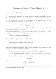
Example: Mixture of 2 normal distributions
Density
0.00 0.05 0.10 0.15 0.20 0.25
0 5 10
y
Figure: λ 1 = (µ 1 = 0, σ 1 = 1), λ 2 = (µ 2 = 7, σ 2 = 0.5), α 1 = 0.7, α 2 = 0.3.
Camila Souza (UBC) Introduction to the EM algorithm November 2010 3 / 25

Maximum likelihood estimator of θ
Our goal is to find ˆθ (i.e., the ˆα j ’s and ˆλ j ’s) that maximizes the
log-likelihood of the data w.r.t. to θ.
log p(y|θ) = log
=
=
n∏
p(y i |θ)
i=1
n∑
log p(y i |θ)
i=1
⎡
⎤
n∑ M∑
log ⎣ α j p j (y i |λ j ) ⎦
i=1
The optimization of this log-likelihood is a complicated task as it involves
the logarithm of a summation.
j=1
Camila Souza (UBC) Introduction to the EM algorithm November 2010 4 / 25

In order to obtain the parameter estimates for this kind of problem it is
common to apply numerical methods such as the EM algorithm.
In this example we can suppose the existence of independent latent
variables z 1 , . . . , z n that tell us from which distribution each y i was
generated from, that is,
y i ∼ p j (y i |θ j ) if z i = j, where p(z i = j) = α j .
Note: It is very common to call y the incomplete data and (y, z) the
complete data.
Camila Souza (UBC) Introduction to the EM algorithm November 2010 5 / 25

or
y i ∼ N(µ 1 , σ 2 1 ) if z i = 1
with p(z = 1) = α 1 = 0.7;
y i ∼ N(µ 2 , σ 2 2 ) if z i = 2
with p(z = 2) = 1 − α 1 .
Density
0.00 0.05 0.10 0.15 0.20 0.25
0 5 10
y
Camila Souza (UBC) Introduction to the EM algorithm November 2010 6 / 25

The EM algorithm
The derivation of the EM algorithm consists of two main steps:
1 Express the log-likelihood in terms of the distribution of latent data;
2 Use this expression to come up with a sequence of θ (k) ’s which will
not decrease log p(y|θ), that is, with
log p(y|θ (k+1) ) ≥ log p(y|θ (k) ).
Note: Various authors have arrived at the EM algorithm while trying to
manipulate the log-likelihood equations to be able to solve them in a nice
way.
Camila Souza (UBC) Introduction to the EM algorithm November 2010 7 / 25

Derivation of the EM algorithm
The joint distribution of y and z (also called the complete data
distribution) can be written as
Rearranging this we get:
Taking the logarithm we have
p(y, z|θ) = p(z|y, θ)p(y|θ).
p(y|θ) =
p(y, z|θ)
p(z|y, θ) .
log p(y|θ) = log p(y, z|θ) − log p(z|y, θ).
Camila Souza (UBC) Introduction to the EM algorithm November 2010 8 / 25

Note that
log p(y|θ) = log p(y, z|θ) − log p(z|y, θ). (1)
holds for any value of z generated according to the distribution p(z|y, θ)
for a chosen value of θ, say θ (k) .
Therefore, the expected value of the right hand side of (1) is also equal to
log p(θ|y).
Camila Souza (UBC) Introduction to the EM algorithm November 2010 9 / 25

Taking the expectation on both sides of the previous equation we have that
∫
log p(y|θ)p(z|y, θ (k) )dz =
∫
∫
log p(y, z|θ)p(z|y, θ (k) )dz −
log p(z|y, θ)p(z|y, θ (k) )dz.
Therefore,
log p(y|θ) = Q(θ, θ (k) ) − H(θ, θ (k) ).
Camila Souza (UBC) Introduction to the EM algorithm November 2010 10 / 25

How can we find a value θ (k+1) so that
log p(y|θ (k+1) ) ≥ log p(y|θ (k) )?
Using log p(y|θ) = Q(θ, θ (k) ) − H(θ, θ (k) ) we have
Q(θ (k+1) , θ (k) ) − Q(θ (k) , θ (k) )
−H(θ (k+1) , θ (k) ) + H(θ (k) , θ (k) ) ≥ 0 (2)
A remarkable result shows that the second line of (2) is non negative for
any θ (k+1) (see McLachlan and Krishnan, 2008).
Thus, we can guarantee that (2) holds if we guarantee that
Q(θ (k+1) , θ (k) ) − Q(θ (k) , θ (k) ) ≥ 0.
Camila Souza (UBC) Introduction to the EM algorithm November 2010 11 / 25

To do that just choose θ (k+1) as the value of θ which maximizes
Q(θ, θ (k) ) for fixed θ (k) . If θ (k+1) is the maximizing value, then
Q(θ (k+1) , θ (k) ) ≥ Q(θ (k) , θ (k) ).
Note: This maximization problem can be a difficult task and it is okay to
choose θ (k+1) that at least does not decrease Q(θ, θ (k) ) from the current
value at θ (k) .
Camila Souza (UBC) Introduction to the EM algorithm November 2010 12 / 25

Therefore, we can guarantee the inequality log p(y|θ (k+1) ) ≥ log p(y|θ (k) )
by choosing
θ (k+1) = arg max Q(θ, θ k ). (3)
θ
Camila Souza (UBC) Introduction to the EM algorithm November 2010 13 / 25

The EM algorithm has two steps:
1 Expectation step (E-step): Q(θ, θ (k) ), the expectation of log p(y, z|θ)
conditional on the data and using the current parameter estimates, is
calculated.
2 Maximization step (M-step): Find θ (k+1) that maximizes Q(θ, θ (k) )
with respect to θ.
Camila Souza (UBC) Introduction to the EM algorithm November 2010 14 / 25

Going back to our example
Remember that our goal is to find ˆθ (i.e., the ˆα j ’s and ˆλ j ’s) that
maximizes the log-likelihood of the data w.r.t. to θ.
log p(y|θ) = log
=
=
n∏
p(y i |θ)
i=1
n∑
log p(y i |θ)
i=1
⎡
⎤
n∑ M∑
log ⎣ α j p j (y i |λ j ) ⎦
i=1
j=1
Camila Souza (UBC) Introduction to the EM algorithm November 2010 15 / 25

Applying the EM algorithm
E-step: Calculate Q(θ, θ (k) ) = E(log p(y, z|θ)|y, θ (k) ).
Note: Maybe a better notation for this expectation would be
E θ (k)(log p(y, z|θ)|y).
The complete data log-likelihood can be written as:
log p(y, z|θ) = log p(y|z, θ) + log p(z|α’s)
=
n∑
n∑
log p(y i |z i , λ zi ) + log α zi
i=1
i=1
= L 1 (λ’s) + L 2 (α’s). (4)
Camila Souza (UBC) Introduction to the EM algorithm November 2010 16 / 25

Since
L 1 (λ’s) =
n∑ M∑
I{z i = j} log p(y i |z i = j, λ j ),
i=1 j=1
where
E(L 1 (λ’s)|y, θ (k) ) =
n∑
i=1 j=1
M∑
p(z i = j|y i , θ (k) ) log p(y i |z i = j, λ j )
p(z i = j|y i , θ (k) p(y i |z i = j, λ (k)
j
) × α (k)
j
) = ∑ J
l=1 p(y i|z i = l, λ (k)
l
) × α (k)
l
Let us use p (k)
ij
as a short notation for p(z i = j|y i , θ (k) ).
Camila Souza (UBC) Introduction to the EM algorithm November 2010 17 / 25

Considering a mixture of normal distributions (λ j = (µ j , σj 2 )) we have:
E(L 1 (λ’s)|y, θ (k) ) = − n 2 log(2π)
− 1 2
− 1 2
n∑
M∑
i=1 j=1
n∑
M∑
i=1 j=1
p (k)
ij
log σj
2
p (k)
ij
(y i − µ j ) 2
.
σ 2 j
Camila Souza (UBC) Introduction to the EM algorithm November 2010 18 / 25

Since
L 2 (α’s) =
n∑ M∑
log α j × I{z i = j}
i=1 j=1
E(L 2 (α’s)|y, θ (k) ) =
=
n∑
i=1 j=1
n∑
i=1 j=1
M∑
log α j × p(z i = j|y i , θ (k) )
M∑
log α j × p (k)
ij
.
Camila Souza (UBC) Introduction to the EM algorithm November 2010 19 / 25

Therefore, considering the normal case, we get:
Q(θ, θ (k) ) = − n 2 log(2π) − 1 2
− 1 2
+
n∑
i=1 j=1
n∑
M∑
i=1 j=1
M∑
n∑
M∑
i=1 j=1
p (k) (y i − µ j ) 2
ji
σj
2
log α j × p (k)
ji
p (k)
ji
log σj
2
Camila Souza (UBC) Introduction to the EM algorithm November 2010 20 / 25

M-sptep: Holding α j and σj
2
we get:
fixed and maximizing Q with respect to µ j
ˆµ j =
∑ n
i=1 y ip (k)
ij
∑ .
n
i=1 p(k) ij
Now holding α j and µ j fixed and maximizing w.r.t. σ 2 j
we have:
ˆσ 2 j =
∑ n
i=1 (y i − µ j ) 2 × p (k)
ij
.
∑i p(k) ij
Camila Souza (UBC) Introduction to the EM algorithm November 2010 21 / 25

And finally in the same way using Lagrange multipliers and the restriction
that ∑ M
j=1 α j = 1 we have:
ˆα j = 1 n
n∑
i=1
p (k)
ij
.
The updates are as follows:
= ˆµ j
σ 2 (k+1)
j
is ˆσ
j 2 with µ j = µ (k+1)
j
;
α (k+1)
j
= ˆα j .
µ (k+1)
j
We iterate the E-step and M-step till convergence.
Camila Souza (UBC) Introduction to the EM algorithm November 2010 22 / 25

In R I found two packages to work with mixture of distributions:
mixdist and mixtools
Camila Souza (UBC) Introduction to the EM algorithm November 2010 23 / 25

References
McLachlan, G. J. and Krishnan, T. (2008), The EM Algorithm and
Extensions, 2nd Ed., John Willey.
Tagare, H. (1998) A gentle introduction to the EM algorithm.
Camila Souza (UBC) Introduction to the EM algorithm November 2010 24 / 25

Thank you !!!
Camila Souza (UBC) Introduction to the EM algorithm November 2010 25 / 25