ILP modeling Exercise 1 – The Steiner Tree Problem

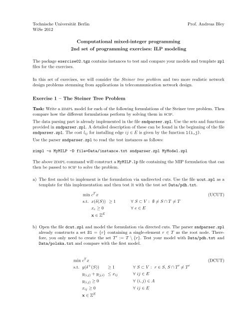
Technische Universität Berlin
WiSe 2012
Prof. Andreas Bley
Computational mixed-integer programming
2nd set of programming exercises: ILP modeling
The package exercise02.tgz contains instances to test and compare your models and template zpl
files for the exercises.
In this set of exercises, we will consider the Steiner tree problem and two more realistic network
design problems stemming from applications in telecommunication network design.
Exercise 1 – The Steiner Tree Problem
Task: Write a zimpl model for each of the following formulations of the Steiner tree problem. Then
compare how the different formulations perform by solving them in scip.
The data parsing part is already implemented in the file sndparser.zpl. Use the sets and functions
provided in sndparser.zpl. A detailed description of these can be found in the beginning of the file
sndparser.zpl. The cost l ij for installing edge ij ∈ E is given by the function l(i,j).
Use the parser sndparser.zpl to read the test instances as follows:
zimpl -o MyMILP -D file=Data/instance.txt sndparser.zpl MyModel.zpl
The above zimpl command will construct a MyMILP.lp file containing the MIP formulation that can
then be passed to scip to solve the problem.
a) The first model to implement is the formulation via undirected cuts. Use the file ucut.zpl as a
template for this implementation and then test it with the test set Data/pdh.txt.
min c T x
s.t. x(δ(S)) ≥ 1
x e ≥ 0
x ∈ Z E
∀ S ⊂ V : ∅ ≠ S ∩ T ≠ T
∀ e ∈ E
(UCUT)
b) Open the file dcut.zpl and model the formulation via directed cuts. The parser sndparser.zpl
already constructs a set S1 = {r} containing a single-element r ∈ T as the root node. Therefore,
you only need to create the set T ′ := T \ {r}. Test your model with Data/pdh.txt and
Data/polska.txt and compare with the first model.
min c T x
s.t. y(δ + (S)) ≥ 1 ∀ S ⊂ V : r ∈ S, S ∩ T ′ ≠ T ′
y (i,j) + y (j,i) ≤ x ij ∀ ij ∈ E
y (i,j) ≥ 0
∀ (i, j) ∈ A
x ij ≥ 0
∀ ij ∈ E
x ∈ Z E
(DCUT)

c) Now implement the (directed) multi-commodity flow formulation using the file mcf.zpl. Solve all
given test instances using this model and check your solutions.
min c T x
s.t.
∑
(i,j)∈δ + (i)
f t (i,j) −
∑
(j,i)∈δ − (i)
f t (j,i)
=
{
1 i = t
0 otherwise
∀ t ∈ T ′ , i ∈ V \ {r}
f s (i,j) + f t (j,i)
≤ x ij ∀ s, t ∈ T ′ , ij ∈ E
f t (i,j) ≥ 0
x ij ≥ 0
x ∈ Z E
∀ t ∈ T ′ , (i, j) ∈ A
∀ ij ∈ E
(MCF)
Optimal solution values
atlanta
cost266
di-yuan
france
nobel-eu
nobel-germany
nobel-us
pdh
polska
4.5550000000e+06
5.6727000000e+05
1.8490000000e+05
1.0608000000e+04
6.9620000000e+04
2.2050000000e+04
5.1290000000e+04
4.8463500000e+05
1.8420000000e+03
Exercise 2 – The Survivable Network Design Problem
Task: Formulate the Survivable Network Design Problem with edge connectivity requirements 1 and
2. Implement and solve your model using zimpl and scip for the given problem instances.
Formally, the Survivable Network Design Problem is given as follows:
{1, 2}-Survivable Network Design Problem
Given
Solution
Goal
undirected graph (V, E) with edge costs l e for the edges e ∈ E together with the connectivity
requests ρ v ∈ {1, 2}
edge set E ′ ⊆ E such that (V, E) contains min{ρ s , ρ t } edge disjoint (s, t)-paths for each
pair of distinct nodes s, t ∈ V .
minimize the total edge cost, i.e. min e∈E ′ l e
All necessary sets and functions are constructed in sndparser.zpl. Assume that
{
2 v ∈ T
ρ v :=
for all v ∈ V .
1 v ∈ V \ T
The cost l ij for installing edge ij is again given by the function l(i,j).
Transform the undirected problem into a problem involving directed paths between the terminals
and use a directed multi-commodity flow formulation similar to that for the Steiner tree problem.
There are several variants to do this. A very good model is obtained as follows (you can use snd.zpl
as a template for this exercise):

1. Pick a root node r ∈ T = {v ∈ V | ρ v = 2} (in zimpl, use the set S1 = {r} created by
sndparser.zpl, again) and create a unit-demand commodity from r to each node in V \ {r}.
These commodities form the first commodity set. Add arc-flow variables and flow conservation
constraints for these commodities.
2. Create a second commodity from r to each node in T \ {r}. These commodities form the
second commodity set. Add extra arc-flow variables and flow conservation constraints for these
commodities, too.
3. Add inequalities to ensure that, for each node t ∈ T \ {r}, the two commodities from r to t are
routed along edge disjoint paths.
4. Create binary variables for each edge and inequalities ensuring that an edge is installed whenever
some commodity flows across the corresponding arcs.
You get a stronger (but also larger) formulation by adding certain flows on anti-parallel arcs.
Optimal solution value
atlanta
cost266
di-yuan
france
nobel-eu
nobel-germany
nobel-us
pdh
polska
1.6095000000e+07
1.7801100000e+06
3.5250000000e+05
3.8932000000e+04
1.5270000000e+05
2.2050000000e+04
2.2050000000e+04
1.0468340000e+06
5.2120000000e+03
Exercise 3 – The Capacitated Network Design Problem
In this exercise, we consider an undirected version of the Capacitated Network Design Problem with
modular edge capacities and edge setup costs given as follows:
Capacitated Network Design Problem
Given
Solution
Goal
undirected graph G = (V, E) with edge setup costs l e capacity u ek and cost c ek for all
edges e ∈ E and all capacity modules k ∈ K
directed commodities C ⊂ V 2 with demands d st for each (s, t) ∈ C
integers y ek for all e ∈ E and k ∈ K such that the edge capacities x e := ∑ k∈K u eky ek
permit a (fractional) multi-commodity flow routing all commodities,
i.e., the edge capacity x ij is at least as large as the sum of the directed flows on the two
arcs (i, j) and (j, i).
minimize the total edge setup cost plus the total capacity installation cost, i.e.
min ∑ e∈E:x l e>0 e + ∑ e∈Ek∈K c eky ek
Task: Formulate the Capacitated Network Design Problem as a mixed-integer linear program. Implement
and solve your model using zimpl and scip for the given problem instances.
All necessary sets and functions are constructed in sndparser.zpl.
To create a correct model, the following steps might be helpful:
1. Add (directed) arc-flow variables and flow conservation constraints for all commodities. Since
theses flows are not going to be aggregated we can interpret every commodity as a unit-demand

commodity.
2. Add inequalities to link the directed flow and the undirected capacity installation variables. If
you used unit-demand commodities as above, you now have to multiply the flow value on each
edge with the corresponding demand and then compare it with the corresponding u ek y ek .
3. Introduce extra binary variables z e for all edges e ∈ E, expressing whether an edge is set up
or not.
These variables can then be used to determine the total edge setup cost.
Some solutions
atlanta
di-yuan
pdh
polska
1.1717500000e+08
2.4304000000e+06
1.2435812000e+07
3.1024000000e+04
Exercise 4 – A realistic extension*
Now adapt your formulation of the Capacitated Network Design Problem in such a way that the
underlying flow problem no longer permits an arbitrary fractional multi-commodity, but enforces a
single-path confluent flow.
In a single-path confluent flow, flow towards a destination can only travel on one arc out of a node.
So, if flows with different origins and a common destination merged in some intermediate node,
then they can never split again and they must continue along the same path towards their common
destination. For each destination, all flows to this destination must form a tree directed towards this
destination.
Formulate your model using a disaggregated formulation for the confluent flow.
Remark: The single-path confluency requirement arises in applications, where the traffic routing is
controlled in an automatic way by (decentralized) routing protocols that, for the sake of simpler
network management, permit only a single outgoing arc towards each destination. Variants of such
protocols are used in telecommunication networks, in postal and logistics networks, and in the freight
car network of Deutsche Bahn, for example.