Projectile Motion Lab Handout - Singhose

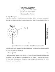
CEDAR GROVE HIGH SCHOOL
Georgia Tech STEP Program
Accelerated Physics – Period 70 – Fall 2004
Mr. Pastirik with Joshua Vaughan
PROJECTILE MOTION LABORATORIES REPORT
In the last two weeks we have explored projectile motion. We have completed two labs which
investigated such motion. In these labs, we investigated the effect of varying the initial height of
the projectile, and, in the second lab, the launch angle of it. We found that the distance a
projectile travels is affected by both. You will now write a lab report that summarizes the results
and compares them to theory. Some information that will help you do this is presented in the
following section. The report expectations, suggested outline, and required formatting are then
presented.
The Theory Behind the Labs
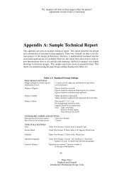
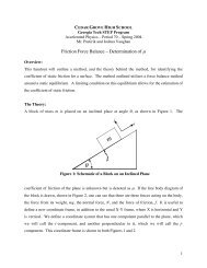
A schematic of the projectile, shown as a point M (you’ll later learn why I choose this letter), at
the instant after firing is shown in Figure 1. The vector V i indicates the initial velocity vector,
while the scalar values of v xi and v yi indicate the horizontal and vertical components of this
vector. The initial height of the projectile, measured from the ground, is indicated by the
variable h. The launch angle is indicated by the variable q.
vyi
Vi
M
q
vxi
h
Figure 1: Schematic of the Dart at the Instant after Launch
1

Using the variables defined in Figure 1 we can find equations that give us the position of the
projectile at any given time (see page 102 of your text for a similar example). They are:
x(t) = v i
cos(q)t (1)
y(t) = - 1 2 gt 2 + v i
sin(q)t + h. (2)
†
†
Let’s examine these equations in the context of each lab.
The First Lab – Distance vs. Launch Height
Notice that, for the first lab, our guns were positioned horizontally, so q was zero. Equations (1)
and (2) then reduce to:
x(t) = v xi
t (3)
y(t) = - 1 2 gt 2 + h. (4)
†
†
†
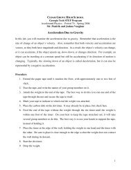
We can solve these equations to find the horizontal distance traveled (in the x direction) for a
given height, h, and initial velocity in the horizontal direction, v xi . We find that:
x(t) = v xi
2h
g
The general trend of this equation, assuming an initial velocity, v xi , of 10
Distance (m)
6.5
6
5.5
5
Distance
†
m
s
(5)
is shown in Figure 2.
4.5
1 1.2 1.4 1.6 1.8 2
Initial Height (m)
Figure 2: Distance vs. Initial Height
2

The Second Lab – Distance vs. Launch Angle
For the second lab, we kept our guns at a constant height, which was very close to the ground.
Because it was held constant, and was small relative to the distance our projectile traveled, we
can ignore it in Equation (2). Equations (1) and (2) then reduce to:
x(t) = v i
cos(q)t (6)
y(t) = - 1 2 gt 2 + v i
sin(q)t. (7)
†
†
†
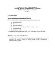
We, just as before, can solve these equations to find a distance traveled (in the x direction). This
time, the result relates the distance to a given initial speed, v i , and the launch angle, q. Notice
that these two parameters can be used to define the initial velocity, V i . We find that:
x(t) = 2v 2 i
cos(q)sin(q)
. (8)
g
The general trend of this equation, assuming an initial velocity, v i , of 10
Distance (m)
12
10
8
6
4
2
Distance
†
m
s
is shown in Figure 3.
0
-2
0 10 20 30 40 50 60 70 80
Launch Angle (deg.)
Figure 3: Distance vs. Launch Angle
The Report
Using the knowledge of projectile motion that you have gained in the last two weeks, and the
information presented above, you will now write a report summarizing the two labs and
contrasting the results obtained with the results that you should expect from theory. In the
3

eport, you should outline the experimental method of each of the labs, and the results obtained
from each. You should then relate these results to the theory. You should, for each experiment,
plot the experimental results and the theoretical results on the same graph. To get as close a fit
as possible, vary the initial velocity in Equations (5) and (8) to get as close an agreement as
possible (remember that this value should be very close to the same for each experiment). In
general, your results will not match the theory exactly. This is okay. You must, however,
explain why this is so. To do this, think about possible sources of error in your experiments,
what assumptions we generally make when talking about projectile motion, and the assumptions
we made in finding Equations (5) and (8) (Hint: in Equation (8), is h actually zero?).
The outline for the report is below:
Title Page
Abstract
This should summarize the results and discussion that are presented in your report, and be
included, at the beginning, on a separate page.
Introduction
This section should introduce (hence the name) the theory behind the experiments. It will
be very similar to the first part of “The Theory Behind the Labs” section of this handout,
including the equations and figure. In this section you should also include a hypothesis
for each experiment and an outline for the rest of your report. This section should
conclude with a sentence of the form.
In the following sections, …
Here the … should include and outline of the sections of your report. This sentence
provides the reader with a roadmap of your report.
Experiment Setup 1
This section describes the first lab setup and procedure. IT DOES NOT PRESENT THE
RESULTS FROM IT.
Experimental Setup 2
This section describes the second lab setup and procedure. IT DOES NOT PRESENT
THE RESULTS FROM IT.
4

Results and Discussion
This is the section where you present the results from your experiments. It should
include the theoretical and actual results (on the same graph) for each experiment. You
should also indicate the value you found for initial velocity in each. You should include
the discussion on the disagreement between the theory and experimental results. Use the
graphs you develop as support.
Conclusion
Very briefly summarizes the results and discussion presented in the report. This is very
similar to the abstract. Contrary to the name, no new information or conclusions are
presented in this section.
Report Guidelines
A template with correct page format can be found on the class website. If you need help
changing these settings, please ask for it. “I didn’t know how to change the settings” is not an
acceptable excuse for incorrect formatting.
Tutorials on how to insert equations, figures, and graphs can also be found on the class website.
If you need help, please ask for it. “I didn’t know how to insert an equation, figure, or graph” is
not an excuse for not having them, or doing them by hand.
1. One report per group will be collected.
2. MAXIMUM page length, not including the title page, abstract, figures, and graphs, is 2
pages. Spelling and grammar should be correct.
3. The report must be computer generated, including figures, graphs, and equations.
4. Text should be 12-point font, Times or Times New Roman, 1.5 line spacing, justified.
5. Page margins should be 1 inch all the way around.
6. Figures and should be numbered and have descriptive captions.
7. Equations should be numbered.
8. When talking about a figure or graph refer to it by number. For example, blah blah blah
is shown in Figure 1. Or, Figure 2 is a plot of blah blah blah. (Replace the blah blah blah
with the actual description of the figure or graph)
9. Cleary indicate sections. Use bold type for the heading. You should space one line
between the previous paragraph and the section heading. (See the section breaks in this
document). Subsections can be indicated by a similar space and italic type.
5