Determining the Concentration of a Solution: Beer's Law
Determining the Concentration of a Solution: Beer's Law
Determining the Concentration of a Solution: Beer's Law

Create successful ePaper yourself
Turn your PDF publications into a flip-book with our unique Google optimized e-Paper software.
<strong>Determining</strong> <strong>the</strong> <strong>Concentration</strong><br />
<strong>of</strong> a <strong>Solution</strong>: Beer’s <strong>Law</strong><br />
DataQuest<br />
21<br />
The primary objective <strong>of</strong> this experiment is to determine <strong>the</strong> concentration <strong>of</strong> an unknown<br />
nickel (II) sulfate solution. You will be using a Colorimeter. The wavelength <strong>of</strong> light used should<br />
be one that is absorbed by <strong>the</strong> solution. The NiSO 4 solution used in this experiment has a deep<br />
green color, so you will use <strong>the</strong> red LED on your Colorimeter. The light striking <strong>the</strong> detector is<br />
reported as absorbance or percent transmittance. A higher concentration <strong>of</strong> <strong>the</strong> colored solution<br />
absorbs more light (and transmits less) than a solution <strong>of</strong> lower concentration.<br />
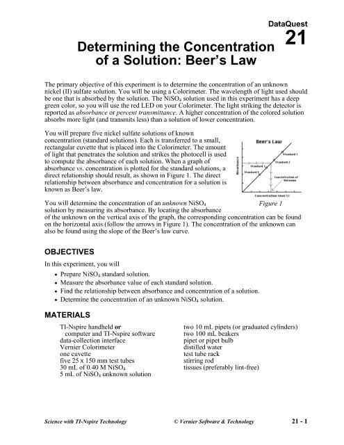
You will prepare five nickel sulfate solutions <strong>of</strong> known<br />
concentration (standard solutions). Each is transferred to a small,<br />
rectangular cuvette that is placed into <strong>the</strong> Colorimeter. The amount<br />
<strong>of</strong> light that penetrates <strong>the</strong> solution and strikes <strong>the</strong> photocell is used<br />
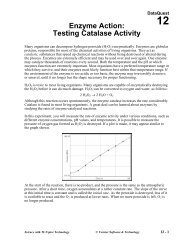
to compute <strong>the</strong> absorbance <strong>of</strong> each solution. When a graph <strong>of</strong><br />
absorbance vs. concentration is plotted for <strong>the</strong> standard solutions, a<br />
direct relationship should result, as shown in Figure 1. The direct<br />
relationship between absorbance and concentration for a solution is<br />
known as Beer’s law.<br />
You will determine <strong>the</strong> concentration <strong>of</strong> an unknown NiSO 4<br />
Figure 1<br />
solution by measuring its absorbance. By locating <strong>the</strong> absorbance<br />
<strong>of</strong> <strong>the</strong> unknown on <strong>the</strong> vertical axis <strong>of</strong> <strong>the</strong> graph, <strong>the</strong> corresponding concentration can be found<br />
on <strong>the</strong> horizontal axis (follow <strong>the</strong> arrows in Figure 1). The concentration <strong>of</strong> <strong>the</strong> unknown can<br />
also be found using <strong>the</strong> slope <strong>of</strong> <strong>the</strong> Beer’s law curve.<br />
OBJECTIVES<br />
In this experiment, you will<br />
• Prepare NiSO 4 standard solution.<br />
• Measure <strong>the</strong> absorbance value <strong>of</strong> each standard solution.<br />
• Find <strong>the</strong> relationship between absorbance and concentration <strong>of</strong> a solution.<br />
• Determine <strong>the</strong> concentration <strong>of</strong> an unknown NiSO 4 solution.<br />
MATERIALS<br />
TI-Nspire handheld or<br />
two 10 mL pipets (or graduated cylinders)<br />
computer and TI-Nspire s<strong>of</strong>tware two 100 mL beakers<br />
data-collection interface<br />
pipet or pipet bulb<br />
Vernier Colorimeter<br />
distilled water<br />
one cuvette<br />
test tube rack<br />
five 25 X 150 mm test tubes<br />
stirring rod<br />
30 mL <strong>of</strong> 0.40 M NiSO 4 tissues (preferably lint-free)<br />
5 mL <strong>of</strong> NiSO 4 unknown solution<br />
Science with TI-Nspire Technology © Vernier S<strong>of</strong>tware & Technology 21 - 1
DataQuest 21<br />
PROCEDURE<br />
1. Obtain and wear goggles. CAUTION: Be careful not to ingest any NiSO 4 solution or spill<br />
any on your skin. Inform your teacher immediately in <strong>the</strong> event <strong>of</strong> an accident.<br />
2. Add about 30 mL <strong>of</strong> 0.40 M NiSO 4 stock solution to a 100 mL beaker. Add about 30 mL <strong>of</strong><br />
distilled water to ano<strong>the</strong>r 100 mL beaker.<br />
3. Label four clean, dry, test tubes 1–4 (<strong>the</strong> fifth solution is <strong>the</strong> beaker <strong>of</strong> 0.40 M NiSO 4 ). Pipet<br />
2, 4, 6, and 8 mL <strong>of</strong> 0.40 M NiSO 4 solution into Test Tubes 1–4, respectively. With a second<br />
pipet, deliver 8, 6, 4, and 2 mL <strong>of</strong> distilled water into Test Tubes 1–4, respectively.<br />
Thoroughly mix each solution with a stirring rod. Clean and dry <strong>the</strong> stirring rod between<br />
stirrings. Keep <strong>the</strong> remaining 0.40 M NiSO 4 in <strong>the</strong> 100 mL beaker to use in <strong>the</strong> fifth trial.<br />
Volumes and concentrations for <strong>the</strong> trials are summarized below:<br />
Trial<br />
number<br />
0.40 M NiSO4<br />
(mL)<br />
Distilled H2O<br />
(mL)<br />
<strong>Concentration</strong><br />
(M)<br />
1 2 8 0.08<br />
2 4 6 0.16<br />
3 6 4 0.24<br />
4 8 2 0.32<br />
5 ~10 0 0.40<br />
4. Prepare a blank by filling an empty cuvette 3/4 full with distilled water. To correctly use a<br />
cuvette, remember:<br />
• All cuvettes should be wiped clean and dry on <strong>the</strong> outside with a tissue.<br />
• Handle cuvettes only by <strong>the</strong> top edge <strong>of</strong> <strong>the</strong> ribbed sides.<br />
• All solutions should be free <strong>of</strong> bubbles.<br />
• Always position <strong>the</strong> cuvette so <strong>the</strong> light passes through <strong>the</strong> clear sides.<br />
5. Connect <strong>the</strong> Colorimeter to <strong>the</strong> data-collection interface. Connect <strong>the</strong> interface to <strong>the</strong><br />
TI-Nspire handheld or computer.<br />
6. Set up <strong>the</strong> data-collection mode and change <strong>the</strong> scale options for <strong>the</strong> graph.<br />
a. Choose New Experiment from <strong>the</strong> Experiment menu. Choose Collection Mode ►<br />
Events with Entry from <strong>the</strong> Experiment menu. Enter <strong>Concentration</strong> as <strong>the</strong> Name and<br />
mol/L as <strong>the</strong> Units. Select OK.<br />
b. Choose Autoscale Settings from <strong>the</strong> Options menu. Select Autoscale from Zero as <strong>the</strong><br />
After Collection setting. Select OK.<br />
7. Calibrate <strong>the</strong> Colorimeter.<br />
a. Place <strong>the</strong> blank in <strong>the</strong> cuvette slot <strong>of</strong> <strong>the</strong> Colorimeter and close <strong>the</strong> lid.<br />
b. Press <strong>the</strong> < or > buttons on <strong>the</strong> Colorimeter to set <strong>the</strong> wavelength to 635 nm (Red). Then<br />
calibrate by pressing <strong>the</strong> CAL button on <strong>the</strong> Colorimeter. When <strong>the</strong> LED stops flashing,<br />
<strong>the</strong> calibration is complete.<br />
21 - 2 Science with TI-Nspire Technology
<strong>Determining</strong> <strong>the</strong> <strong>Concentration</strong> <strong>of</strong> a <strong>Solution</strong>: Beer’s <strong>Law</strong><br />
8. You are now ready to collect absorbance-concentration data for <strong>the</strong> five standard solutions.<br />
a. Start data collection ( ).<br />
b. Empty <strong>the</strong> water from <strong>the</strong> cuvette. Using <strong>the</strong> solution in Test Tube 1, rinse <strong>the</strong> cuvette<br />
twice with ~1 mL amounts and <strong>the</strong>n fill it 3/4 full. Wipe <strong>the</strong> outside with a tissue and<br />
place it in <strong>the</strong> Colorimeter. Close <strong>the</strong> lid.<br />
c. When <strong>the</strong> value displayed on <strong>the</strong> screen has stabilized, click <strong>the</strong> Keep button ( ) and<br />
enter 0.080 as <strong>the</strong> concentration in mol/L. Select OK. The absorbance and concentration<br />
values have now been saved for <strong>the</strong> first solution.<br />
d. Discard <strong>the</strong> cuvette contents as directed by your instructor. Using <strong>the</strong> solution in Test<br />
Tube 2, rinse <strong>the</strong> cuvette twice with ~1 mL amounts, and <strong>the</strong>n fill it 3/4 full. Place <strong>the</strong><br />
cuvette in <strong>the</strong> Colorimeter and close <strong>the</strong> lid. Wait for <strong>the</strong> value displayed on <strong>the</strong> screen to<br />
stabilize and click <strong>the</strong> Keep button ( ). Enter 0.16 as <strong>the</strong> concentration in mol/L. Select<br />
OK.<br />
e. Repeat <strong>the</strong> procedure for Test Tube 3 (0.24 M) and Test Tube 4 (0.32 M), as well as <strong>the</strong><br />
stock 0.40 M NiSO 4 . Note: Wait until Step 10 to test <strong>the</strong> unknown.<br />
f. Stop data collection ( ).<br />
g. Click <strong>the</strong> Table View tab ( ) to display <strong>the</strong> data table. Record <strong>the</strong> absorbance and<br />
concentration data values in your data table.<br />
9. Display a graph <strong>of</strong> absorbance vs. concentration with a linear regression curve.<br />
a. Click <strong>the</strong> Graph View tab ( ).<br />
b. Choose Curve Fit ► Linear from <strong>the</strong> Analyze menu. The linear-regression statistics<br />
for <strong>the</strong>se two data columns are displayed for <strong>the</strong> equation in <strong>the</strong> form<br />
y = mx + b<br />
where x is concentration, y is absorbance, m is <strong>the</strong> slope, and b is <strong>the</strong> y-intercept.<br />
c. Record your fit equation in your data table.<br />
Note: One indicator <strong>of</strong> <strong>the</strong> quality <strong>of</strong> your data is <strong>the</strong> size <strong>of</strong> b. It is a very small value if<br />
<strong>the</strong> regression line passes through or near <strong>the</strong> origin. The correlation coefficient, r,<br />
indicates how closely <strong>the</strong> data points match up with (or fit) <strong>the</strong> regression line. A value <strong>of</strong><br />
1.00 indicates a nearly perfect fit. The graph should indicate a direct relationship between<br />
absorbance and concentration, a relationship known as Beer’s law. The regression line<br />
should closely fit <strong>the</strong> five data points and pass through (or near) <strong>the</strong> origin <strong>of</strong> <strong>the</strong> graph.<br />
10. Determine <strong>the</strong> absorbance value <strong>of</strong> <strong>the</strong> unknown NiSO 4 solution.<br />
a. Click <strong>the</strong> Meter View tab ( ).<br />
b. Obtain about 5 mL <strong>of</strong> <strong>the</strong> unknown NiSO 4 in ano<strong>the</strong>r clean, dry, test tube. Record <strong>the</strong><br />
number <strong>of</strong> <strong>the</strong> unknown in your data table.<br />
c. Rinse <strong>the</strong> cuvette twice with <strong>the</strong> unknown solution and fill it about 3/4 full. Wipe <strong>the</strong><br />
outside <strong>of</strong> <strong>the</strong> cuvette and place it into <strong>the</strong> device.<br />
d. Monitor <strong>the</strong> absorbance value. When this value has stabilized, record it in your data table.<br />
11. Discard <strong>the</strong> solutions as directed by your instructor.<br />
Science with TI-Nspire Technology 21 - 3
DataQuest 21<br />
DATA<br />
Trial<br />
<strong>Concentration</strong><br />
(mol/L)<br />
Absorbance<br />
1 0.080<br />
2 0.16<br />
3 0.24<br />
4 0.32<br />
5 0.40<br />
6 Unknown number ____<br />
Linear Fit Equation: y = mx + b<br />
<strong>Concentration</strong> <strong>of</strong> unknown (mol/L)<br />
PROCESSING THE DATA<br />
1. To determine <strong>the</strong> concentration <strong>of</strong> <strong>the</strong> unknown NiSO 4 solution, interpolate along <strong>the</strong><br />
regression line to convert <strong>the</strong> absorbance value <strong>of</strong> <strong>the</strong> unknown to concentration.<br />
a. Click <strong>the</strong> Graph View tab ( ).<br />
b. Choose Interpolate from <strong>the</strong> Analyze menu.<br />
c. Click on any point on <strong>the</strong> regression curve. Use ► and ◄ to find <strong>the</strong> Linear Fit value that<br />
is closest to <strong>the</strong> absorbance reading you obtained in Step 10. The corresponding NiSO 4<br />
concentration, in mol/L, will be displayed.<br />
d. Record <strong>the</strong> concentration value in your data table.<br />
2. (optional) Print a graph <strong>of</strong> absorbance vs. concentration, with a regression line and<br />
interpolated unknown concentration displayed.<br />
21 - 4 Science with TI-Nspire Technology