Data Mining Methods and Models

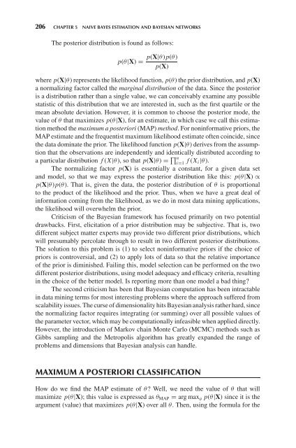
206 CHAPTER 5 NAIVE BAYES ESTIMATION AND BAYESIAN NETWORKS
The posterior distribution is found as follows:
p(θ|X) = p(X|θ)p(θ)
p(X)
where p(X|θ) represents the likelihood function, p(θ) the prior distribution, and p(X)
a normalizing factor called the marginal distribution of the data. Since the posterior
is a distribution rather than a single value, we can conceivably examine any possible
statistic of this distribution that we are interested in, such as the first quartile or the
mean absolute deviation. However, it is common to choose the posterior mode, the
value of θ that maximizes p(θ|X), for an estimate, in which case we call this estimation
method the maximum a posteriori (MAP) method. For noninformative priors, the
MAP estimate and the frequentist maximum likelihood estimate often coincide, since
the data dominate the prior. The likelihood function p(X|θ) derives from the assumption
that the observations are independently and identically distributed according to
a particular distribution f (X|θ), so that p(X|θ) = � n
i=1
f (Xi|θ).
The normalizing factor p(X) is essentially a constant, for a given data set
and model, so that we may express the posterior distribution like this: p(θ|X) ∝
p(X|θ)p(θ). That is, given the data, the posterior distribution of θ is proportional
to the product of the likelihood and the prior. Thus, when we have a great deal of
information coming from the likelihood, as we do in most data mining applications,
the likelihood will overwhelm the prior.
Criticism of the Bayesian framework has focused primarily on two potential
drawbacks. First, elicitation of a prior distribution may be subjective. That is, two
different subject matter experts may provide two different prior distributions, which
will presumably percolate through to result in two different posterior distributions.
The solution to this problem is (1) to select noninformative priors if the choice of
priors is controversial, and (2) to apply lots of data so that the relative importance
of the prior is diminished. Failing this, model selection can be performed on the two
different posterior distributions, using model adequacy and efficacy criteria, resulting
in the choice of the better model. Is reporting more than one model a bad thing?
The second criticism has been that Bayesian computation has been intractable
in data mining terms for most interesting problems where the approach suffered from
scalability issues. The curse of dimensionality hits Bayesian analysis rather hard, since
the normalizing factor requires integrating (or summing) over all possible values of
the parameter vector, which may be computationally infeasible when applied directly.
However, the introduction of Markov chain Monte Carlo (MCMC) methods such as
Gibbs sampling and the Metropolis algorithm has greatly expanded the range of
problems and dimensions that Bayesian analysis can handle.
MAXIMUM A POSTERIORI CLASSIFICATION
How do we find the MAP estimate of θ? Well, we need the value of θ that will
maximize p(θ|X); this value is expressed as θMAP = arg max θ p(θ|X) since it is the
argument (value) that maximizes p(θ|X) over all θ. Then, using the formula for the