REP SFCG 32-2R1 (Sharing between RNSS & EESS in 1215-1300 ...
REP SFCG 32-2R1 (Sharing between RNSS & EESS in 1215-1300 ...
REP SFCG 32-2R1 (Sharing between RNSS & EESS in 1215-1300 ...

You also want an ePaper? Increase the reach of your titles
YUMPU automatically turns print PDFs into web optimized ePapers that Google loves.
Space Frequency<br />
Coord<strong>in</strong>ation Group<br />
Report <strong>SFCG</strong> <strong>32</strong>-<strong>2R1</strong><br />
Abstract<br />
SHARING BETWEEN <strong>RNSS</strong> AND <strong>EESS</strong> (ACTIVE)<br />
IN THE <strong>1215</strong>-<strong>1300</strong> MHZ BAND<br />
This report presents an analysis of the shar<strong>in</strong>g <strong>between</strong> <strong>RNSS</strong> and <strong>EESS</strong> (active) <strong>in</strong> the<br />
<strong>1215</strong>-<strong>1300</strong> MHz band. The report presents the results of compatibility measurements and<br />
possible compatibility measures <strong>between</strong> systems <strong>in</strong> the <strong>EESS</strong> (active) and systems <strong>in</strong> the <strong>RNSS</strong><br />
<strong>in</strong> the band <strong>1215</strong>-<strong>1300</strong> MHz.<br />
3-July-2013 Page 1 of 21 <strong>REP</strong> <strong>SFCG</strong> <strong>32</strong>-<strong>2R1</strong>
TABLE OF CONTENTS<br />
1. Introduction .......................................................................................................................... 3<br />
2. Measurement of Degradation Ratio of GPS Receiver from Scatterometer2 and SAR3<br />
Systems ........................................................................................................................... 3<br />
2.1. Compatibility Measurement Approach ................................................................... 3<br />
2.2. Synthetic Aperture radar (SAR3) and Scatterometer2 signals ................................ 3<br />
2.3. SAR and Scatterometer Signal Calibration ............................................................. 8<br />
2.4. <strong>RNSS</strong> receiver characteristics and performance criteria ......................................... 9<br />
2.5. Measurement procedure .......................................................................................... 9<br />
2.6. Measurement results ................................................................................................ 9<br />
2.6.1 Receiver Selectivity and Antenna Filter ............................................. 9<br />
2.6.2 C/N 0 or SNR Degradation Equation .................................................. 13<br />
2.6.3 Measured SNR or C/N 0 Degradation versus Effective Duty Cycle .... 13<br />
2.7. Possible Mitigation Measures.................................................................................. 15<br />
2.7.1 Reduction of the Ratio of Chirp Bandwidth Overlapp<strong>in</strong>g the Pre-<br />
Correlator Band .................................................................................... 15<br />
2.7.2 Reduction of the Ratio of Observation Time per Cycle ............................ 15<br />
2.8. Conclusions related to the GPS receiver protection ................................................ 16<br />
3 Measurement of Degradation Ratio of QZSS Receivers from ALOS-2 SAR System ......... 20<br />
4 Conclusion ............................................................................................................................ 21<br />
3-July-2013 Page 2 of 21 <strong>REP</strong> <strong>SFCG</strong> <strong>32</strong>-<strong>2R1</strong>
1. Introduction<br />
This report presents results of compatibility measurements and possible compatibility measures<br />
<strong>between</strong> systems <strong>in</strong> the <strong>EESS</strong> (active) and systems <strong>in</strong> the <strong>RNSS</strong> <strong>in</strong> the band <strong>1215</strong>-<strong>1300</strong> MHz.<br />
2. Measurement of Degradation Ratio of GPS Receiver from Scatterometer2 and SAR3<br />
Systems<br />
2.1. Compatibility Measurement Approach<br />
Parametric measurements were conducted for several SAR and scatterometer signal<br />
characteristics, pulse widths, PRFs and chirps. The SAR and scatterometer signals were hardcoupled<br />
<strong>in</strong>to the <strong>RNSS</strong> receiver and the receiver performance was monitored and the SNR or<br />
C/N 0 was recorded as a function of the effective duty cycle at the receiver.<br />
2.2. Synthetic Aperture radar (SAR3) and Scatterometer2 signals<br />
The SAR3 system is a 1.26 GHz, synthetic aperture radar designed to acquire <strong>in</strong>terferometric<br />
radar backscatter signals to monitor the Earth’s deform<strong>in</strong>g surfaces. The spaceborne radar is<br />
designed to operate at an altitude of 757 km and <strong>in</strong>cl<strong>in</strong>ation of 98 deg to provide an average<br />
revisit time of 13 to 15 days. SAR3 has several modes with correspond<strong>in</strong>g waveforms. One of<br />
the waveforms consists of a split spectrum with 20 MHz at one end of the 85 MHz allowed<br />
transmission and 5 MHz at the opposite end <strong>in</strong> order to mitigate the effects of the ionosphere on<br />
the <strong>in</strong>terferometric phase. SAR3 has a reflector fed antenna with an active array feed. The active<br />
array feed consists of a s<strong>in</strong>gle str<strong>in</strong>g set of 8-24 transmit/receive (T/R) modules that both<br />
transmit and receive both horizontal and vertical polarizations. Echoes received at the T/R<br />
modules are immediately digitized and digital beamform<strong>in</strong>g techniques are employed to achieve<br />
the desired illum<strong>in</strong>ation while reduc<strong>in</strong>g downl<strong>in</strong>k data rate. Table 1 summarizes the test<br />
characteristics of the SAR3 radar and antenna as simulated for the compatibility tests and<br />
analysis. The mode designations such as “SAR3-3” correspond to those test modes as shown <strong>in</strong><br />
Table 3.<br />
3-July-2013 Page 3 of 21 <strong>REP</strong> <strong>SFCG</strong> <strong>32</strong>-<strong>2R1</strong>
Table 1 Test characteristics of SAR3 Radar and Antenna<br />
Parameters SAR3-3 SAR3-4 SAR3-6 SAR3-8<br />
Orbit altitude, km 757<br />
Orbit <strong>in</strong>cl<strong>in</strong>ation, deg 98<br />
Local time of ascend<strong>in</strong>g node<br />
(LAN) 18:00<br />
Transmit (Xmt) pk pwr, W 3 200<br />
Antenna pk xmt ga<strong>in</strong>, dBi 33.4<br />
e.i.r.p. pk, dBW 68.5<br />
Antenna pk rcv ga<strong>in</strong>, dBi 41<br />
Antenna xmt elev. beamwidth, deg 15<br />
Antenna xmt az. beamwidth, deg 0.8<br />
Antenna rcv elev. beamwidth, deg 16.7<br />
Antenna rcv az. beamwidth, deg 0.8<br />
RF centre frequency, MHz 1 220.0 + 1 287.5 1 227.5 + 1 295.0 1 257.5 1 257.5<br />
Polarization<br />
RF bandwidth, MHz<br />
5 + 20<br />
(split spectrum)<br />
Dual/quad, l<strong>in</strong>ear H and V<br />
20 + 5<br />
40 78<br />
(split spectrum)<br />
RF pulsewidth, µsec 5 + 20 20 + 5 40 50<br />
Pulse repetition frequency max,<br />
Hz 3 500<br />
Xmt Ave. pwr, W 240 240 448 560<br />
e.i.r.p. ave, dBW 57.4 57.4 59.9 60.9<br />
Chirp rate, MHz/µsec 1.0 1.0 1.0 1.56<br />
Xmt duty cycle, % 8.75 8.75 14.0 17.5<br />
Azimuth (Az) scan rate, rpm 0<br />
Antenna beam xmt look angle, deg 35<br />
Antenna beam rcv look angle, deg 35<br />
Antenna beam xmt az angle, deg 0<br />
Antenna beam rcv az angle, deg 0<br />
System noise temp, deg 420<br />
Scatterometer 2 is a 1.26 GHz radar designed to acquire radar backscatter signals to estimate<br />
surface soil moisture. The spaceborne radar is designed to operate at an altitude of 685 km and<br />
<strong>in</strong>cl<strong>in</strong>ation of 98 deg to provide an average revisit time of 3 days for soil moisture globally. The<br />
orbit is dawn/dusk sun-synchronous. The radar will collect dual polarimetric returns (VV, HH,<br />
3-July-2013 Page 4 of 21 <strong>REP</strong> <strong>SFCG</strong> <strong>32</strong>-<strong>2R1</strong>
and HV transmit-receive polarizations) at 3 km spatial resolution. In order to m<strong>in</strong>imize<br />
range/Doppler ambiguities with the basel<strong>in</strong>e antenna and view<strong>in</strong>g geometry, separate carrier<br />
frequencies are used for each polarization (e.g. 1260 MHz for H-pol and 1263 MHz for V-pol).<br />
The sub- band center frequencies are set 3 MHz apart, and the two frequencies can be selectively<br />
set with<strong>in</strong> the 80 MHz range of 1217.5-1297.5 MHz to m<strong>in</strong>imize RFI. The l<strong>in</strong>early FM pulses<br />
will have a pulse duration of 15 microseconds and bandwidth of 1 MHz. Table 2 summarizes the<br />
characteristics of the Scatterometer 2 radar and antenna as simulated for the compatibility tests<br />
and analysis. The mode designations such as “SCAT2-1” correspond to those test modes as<br />
shown <strong>in</strong> Table 3.<br />
Table 2 Test characteristics of Scatterometer 2 Radar and Antenna<br />
Parameters SCAT2-1 SCAT2-2<br />
Orbit altitude, km 685<br />
Orbit <strong>in</strong>cl<strong>in</strong>ation, deg 98<br />
Local time of ascend<strong>in</strong>g node<br />
(LAN) 18:00<br />
Xmt pk pwr, W<br />
<strong>32</strong>0 maximum (230-300 typical) per polarization<br />
Antenna pk xmt ga<strong>in</strong>, dBi 36<br />
e.i.r.p. peak, dBW 61.0<br />
Antenna xmt elev. beamwidth,<br />
deg 2.6<br />
Antenna xmt az. beamwidth, deg 2.6<br />
RF centre frequency, MHz 1 227.6 MHz 1 295.5<br />
Polarization<br />
Dual, l<strong>in</strong>ear H and V<br />
RF bandwidth, MHz 2 x 1<br />
RF pulsewidth, µsec 2 x 15<br />
Pulse repetition frequency max,<br />
Hz 1750<br />
Xmt Ave. pwr, W 16.8<br />
e.i.r.p. ave, dBW 48.25<br />
Chirp rate, MHz/µsec 0.35<br />
Xmt duty cycle, % 5.25<br />
Azimuth (Az) scan rate, rpm 14.6<br />
Antenna beam xmt look angle,<br />
deg 35.5<br />
Antenna beam xmt az angle, deg 0-360<br />
3-July-2013 Page 5 of 21 <strong>REP</strong> <strong>SFCG</strong> <strong>32</strong>-<strong>2R1</strong>
A SAR and scatterometer signal simulator used different comb<strong>in</strong>ations of the follow<strong>in</strong>g<br />
waveform characteristics:<br />
Pulse width: 5 µs, 15 µs, 20 µs, 40 µs and 50 µs<br />
Chirp bandwidth:<br />
Pulse Repetition Rate (PRR):<br />
Signal levels:<br />
1 MHz, 5 MHz, 20 MHz, 40 MHz and 78 MHz<br />
1750 Hz and 3500 Hz<br />
-125 dBW, -105 dBW, -85 dBW, and -75 dBW<br />
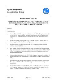
Figure 1 shows a block diagram of the equipment to generate the SAR and scatterometer<br />
waveforms. For the scatterometer waveforms, there was a gat<strong>in</strong>g circuit to turn the signal on for<br />
100 – 200 msec to simulate the transit of the scatterometer antenna beam rotat<strong>in</strong>g through the<br />
<strong>RNSS</strong> antenna beam pattern and to turn the signal off for 4 seconds to simulate the antenna<br />
rotation period of 4.1 seconds. The spaceborne SAR looks off to the side of the spacecraft at a<br />
fixed angle<br />
Figure 1a Test Setup with <strong>RNSS</strong> Simulator <strong>in</strong> Laboratory<br />
The SAR and scatterometer signals were hard-coupled <strong>in</strong>to the RF front-end of the <strong>RNSS</strong><br />
receiver just after the antenna. SAR and scatterometer waveforms were monitored with a<br />
spectrum analyzer, oscilloscope and peak power meter at the <strong>in</strong>put to the <strong>RNSS</strong> receiver RF<br />
stage.<br />
3-July-2013 Page 6 of 21 <strong>REP</strong> <strong>SFCG</strong> <strong>32</strong>-<strong>2R1</strong>
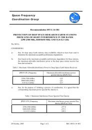
The peak <strong>in</strong>terfer<strong>in</strong>g signal levels to the <strong>RNSS</strong> ground receiver are calculated from the<br />
Scatterometer 2 at nom<strong>in</strong>al altitude of 685 km. In Figure 2a, there are “spikes” of RFI occurr<strong>in</strong>g<br />
every 4.1 seconds as the Scatterometer 2 antenna beam rotates <strong>in</strong> azimuth toward the <strong>RNSS</strong><br />
receiver. Figure 2a also shows below a span of 8 seconds <strong>in</strong> the orbit for two of the maximum<br />
‘spikes’, and the temporal half-power width of the spikes are about 30 milliseconds. The shapes<br />
of the spikes are the modulation by the Scatterometer 2 antenna pattern <strong>in</strong> azimuth as the beam<br />
Figure 1b Test Setup with <strong>RNSS</strong> Satellite Transmissions on Roof of Build<strong>in</strong>g<br />
rotates at 14.6 rpm. The peak RFI levels vary from -170 dBW at the low elevation angles at the<br />
beg<strong>in</strong>n<strong>in</strong>g and end of the pass to about -90 dBW at 50 deg elevation angle when the<br />
Scatterometer 2 antenna beam center aligns with the <strong>RNSS</strong> receiver.<br />
Figure 2b shows the RFI levels from SAR3 <strong>in</strong>to a terrestrial <strong>RNSS</strong> receiver as a function of time<br />
dur<strong>in</strong>g a typical pass. There is a s<strong>in</strong>gle “spike” at the maximum elevation angle as the SAR3<br />
antenna is po<strong>in</strong>ted starboard and perpendicular to the ground nadir track toward the <strong>RNSS</strong><br />
receiver. SAR3’s antenna beamwidth <strong>in</strong> azimuth is 0.8 deg result<strong>in</strong>g <strong>in</strong> a duration of the RFI<br />
“spike” of about 2 seconds <strong>in</strong> the footpr<strong>in</strong>t and has a peak RFI level -82 dBW RFI levels vary<br />
from -216 dBW at the low elevation angles at the beg<strong>in</strong>n<strong>in</strong>g of the pass and <strong>in</strong>crease to above -<br />
135 dBW, a typical receiver noise level for a <strong>RNSS</strong> receiver, and susta<strong>in</strong> that level or higher for<br />
more than 250 seconds.<br />
3-July-2013 Page 7 of 21 <strong>REP</strong> <strong>SFCG</strong> <strong>32</strong>-<strong>2R1</strong>
(a) Scatterometer 2 (b) SAR 3<br />
Figure 2 Scatterometer 2 and SAR3 RFI Levels <strong>in</strong>to <strong>RNSS</strong> Receiver over Typical Pass<br />
2.3. SAR and Scatterometer Signal Calibration<br />
The SAR and scatterometer signal simulator was calibrated to establish a prescribed signal level<br />
at the <strong>RNSS</strong> receiver <strong>in</strong>put. The <strong>in</strong>terference level of the generated waveform was measured at<br />
the <strong>in</strong>put to the coupler us<strong>in</strong>g a peak power meter and monitored on a spectrum analyzer.<br />
Known values of attenuators were <strong>in</strong>serted to atta<strong>in</strong> the desired <strong>in</strong>terference level <strong>in</strong>to the <strong>RNSS</strong><br />
receiver. Interference signals were split to both <strong>RNSS</strong> receivers under test to allow parallel<br />
test<strong>in</strong>g of both receivers.<br />
3-July-2013 Page 8 of 21 <strong>REP</strong> <strong>SFCG</strong> <strong>32</strong>-<strong>2R1</strong>
2.4. <strong>RNSS</strong> receiver characteristics and performance criteria<br />
Recommendation ITU-R M.1902 has the characteristics and protection criteria for <strong>RNSS</strong><br />
receivers. Table 1-1 of Annex 1 lists seven <strong>RNSS</strong> receivers, two of which were <strong>in</strong>cluded <strong>in</strong> the<br />
compatibility tests: the SBAS ground reference receiver <strong>RNSS</strong>1, and high precision semicodeless<br />
<strong>RNSS</strong>2.<br />
The follow<strong>in</strong>g <strong>RNSS</strong> receiver performance parameters were monitored dur<strong>in</strong>g the measurements<br />
to evaluate the effects of active spaceborne radar pulsed emissions on the system performance:<br />
a. Decrease <strong>in</strong> SNR<br />
b. Decrease <strong>in</strong> C/N 0<br />
The objective of the data analysis was to determ<strong>in</strong>e the amount of degradation of the signal-tonoise<br />
ratio (SNR) or C/N 0 observed by the <strong>RNSS</strong> receiver <strong>in</strong> the presence of the <strong>in</strong>terfer<strong>in</strong>g radar<br />
signal.<br />
2.5. Measurement procedure<br />
Several parameters of the <strong>in</strong>terfer<strong>in</strong>g signal are varied <strong>in</strong> the different tests, <strong>in</strong>clud<strong>in</strong>g the radar<br />
type (SAR and scatterometer), power level, frequency, and gat<strong>in</strong>g so that the degradation varies<br />
accord<strong>in</strong>gly. Each test consists of a number (rang<strong>in</strong>g from two to ten) of 100-s <strong>in</strong>tervals <strong>in</strong> which<br />
the <strong>in</strong>terfer<strong>in</strong>g signal is alternately off and on. With<strong>in</strong> each 100-second <strong>in</strong>terval there are ten 10-<br />
second measurements of the voltage SNR of the L2P signal for as many as twelve <strong>RNSS</strong><br />
satellites.<br />
2.6. Measurement results<br />
2.6.1 Receiver Selectivity and Antenna Filter<br />
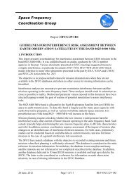
The portion of the received <strong>in</strong>terference power conta<strong>in</strong>ed with the <strong>RNSS</strong> pre-correlator band can<br />
be calculated by multiply<strong>in</strong>g the <strong>in</strong>terference waveform spectrum by the comb<strong>in</strong>ed filter response<br />
of the receiver sensitivity and the antenna filter/pre-amplifier. The comb<strong>in</strong>ed filter response of<br />
the receiver sensitivity and the antenna filter/pre-amplifier is shown <strong>in</strong> Figure 3. The<br />
<strong>in</strong>terference waveform spectra are shown <strong>in</strong> Figure 4 for the n<strong>in</strong>e configurations. The product of<br />
the <strong>in</strong>terference waveform spectra and the comb<strong>in</strong>ed filter response are shown <strong>in</strong> Figure 5 for the<br />
n<strong>in</strong>e configurations. Table 3 shows the pulse-width, PRF, bandwidth, and center RF frequency<br />
for the different scatterometer and SAR configurations.<br />
3-July-2013 Page 9 of 21 <strong>REP</strong> <strong>SFCG</strong> <strong>32</strong>-<strong>2R1</strong>
Response dB<br />
0<br />
-10<br />
-20<br />
-30<br />
-40<br />
-50<br />
-60<br />
-70<br />
-80<br />
-90<br />
-100<br />
-110<br />
-120<br />
BlackJackselectivity +<br />
-130<br />
<strong>RNSS</strong>1 selectivity+filter/pre-amp<br />
filter/pre-amp<br />
-140<br />
<strong>RNSS</strong>2 selectivity+filter/pre-amp<br />
-150<br />
Specified Reference<br />
-160<br />
Specified Filter 4 dB/MHz reference filter 4 dB/MHz<br />
-170<br />
-180<br />
<strong>1215</strong> 1220 1225 1230 1235 1240 1245 1250 1255 1260 1265 1270 1275 1280 1285 1290 1295 <strong>1300</strong><br />
Frequency MHz<br />
Figure 3 Total Filter Response for <strong>RNSS</strong>1 and <strong>RNSS</strong>2 Receivers<br />
3-July-2013 Page 10 of 21 <strong>REP</strong> <strong>SFCG</strong> <strong>32</strong>-<strong>2R1</strong>
a) SCAT2-1 a) SCAT2-1 b) SCAT2-2 b) SCAT2-2 c) SAR3-3 c) SAR3-3<br />
d) SAR3-4<br />
e) SAR3-5 f) SAR3-6<br />
d) SAR3-4<br />
e) SAR3-5 f) SAR3-6<br />
g) SAR3-7 h) SAR3-8<br />
h) UAVSAR-9<br />
Figure 4 Relative Spectral Power over <strong>1215</strong>-<strong>1300</strong> MHz Band for Interference Waveforms<br />
3-July-2013 Page 11 of 21 <strong>REP</strong> <strong>SFCG</strong> <strong>32</strong>-<strong>2R1</strong>
.<br />
a) SCAT2-1 b) SCAT2-2<br />
c) SAR3-3<br />
d) SAR3-4<br />
e) DESDynI-5 SAR3-5<br />
f) DESDynI-6 SAR3-6<br />
g) SAR3-7 h) SAR3-8<br />
Figure 5 Received Spectral Power over <strong>1215</strong>-<strong>1300</strong> MHz Band for Interference Waveforms<br />
i) SAR3-9<br />
3-July-2013 Page 12 of 21 <strong>REP</strong> <strong>SFCG</strong> <strong>32</strong>-<strong>2R1</strong>
2.6.2 C/N 0 or SNR Degradation Equation<br />
For some <strong>EESS</strong> (active) scatterometers operat<strong>in</strong>g <strong>in</strong> sun-synchronous orbit, the degradation to<br />
the SNR or carrier-to-noise density can be approximated by the follow<strong>in</strong>g equation:<br />
∆SNR = 20log(1<br />
− PDCLIM<br />
)<br />
(1)<br />
PDC = ( τ<br />
,<br />
+ τ ) PRF<br />
(2)<br />
LIM<br />
PW EFF<br />
RT<br />
EFF<br />
τ = τ<br />
PW , EFF<br />
PW<br />
BW overlap<br />
BW<br />
(3)<br />
PRF<br />
EFF<br />
τ<br />
obs<br />
= PRF<br />
(4)<br />
T<br />
TC<br />
where:<br />
PDC LIM : fractional duty cycle of the saturat<strong>in</strong>g pulses (unitless ratio);<br />
τ PW,EFF : the effective pulse width ,<br />
τ RT : the <strong>RNSS</strong> recovery time (0.6 µsec for <strong>RNSS</strong>1),<br />
PRF EFF : the effective pulse repetition frequency,<br />
τ obs : the observation time per cycle that the received peak power is above the<br />
<strong>RNSS</strong> <strong>in</strong>put compression po<strong>in</strong>t (100-300 millisec for SCATTEROMETER<br />
2), and<br />
T TC :<br />
τ PW :<br />
the cycle time or time constant (4.1 sec rotation period for<br />
SCATTEROMETER 2),<br />
the transmit pulse width (µsec)<br />
PRF: the transmit pulse repetition frequency (e.g. PRF= 3500 Hz) ,<br />
BW overlap :<br />
BW:<br />
the portion of the bandwidth which overlaps the <strong>RNSS</strong> L2 pre-correlator<br />
RF/IF band centered at 1227.6 MHz (MHz);<br />
the pre-correlator RF/IF bandwidth (MHz);<br />
2.6.3 Measured SNR or C/N 0 Degradation versus Effective Duty Cycle<br />
Us<strong>in</strong>g the equations above for the effective duty cycle, dc eff , or the fractional duty cycle PDC LIM<br />
as <strong>in</strong> equation (2) above, the measured SNR or C/N 0 degradation is plotted versus the dc eff as<br />
shown <strong>in</strong> Figure 3. Regions of measured values of degradation can be dist<strong>in</strong>guished <strong>between</strong><br />
that for gat<strong>in</strong>g “ON” and gat<strong>in</strong>g “OFF”. The measured degradation values are clustered around<br />
the trendl<strong>in</strong>e curve of 20 log (1-dc eff ).<br />
3-July-2013 Page 13 of 21 <strong>REP</strong> <strong>SFCG</strong> <strong>32</strong>-<strong>2R1</strong>
Test results for all the tests conducted are listed <strong>in</strong> Table 3. This table represents as-run test<br />
parameters and test results. Explanation of the entries <strong>in</strong> Table 3 is as follows:<br />
Col. 1 Conta<strong>in</strong>s the test number <strong>in</strong> the format (day number)-(sequence number). Day 1 is June<br />
22, 2010, and day 4 is June 25. Also, ‘roof” or “sim” <strong>in</strong>dicates whether the test was<br />
conducted us<strong>in</strong>g signals from an antenna on the roof or from the <strong>RNSS</strong> constellation<br />
simulator.<br />
Col. 2 Gives the type of radar signal (SCAT2 or SAR3) and a configuration number (from 1 to<br />
8). The configuration number is <strong>in</strong>tended to refer to a specific set of the parameters <strong>in</strong><br />
columns 3 through 6.<br />
Col. 3 Gives the pulse repetition frequency (PRF) <strong>in</strong> Hz and the pulse length or duration of each<br />
pulse <strong>in</strong> µs. SAR3 waveforms often consist of split spectrum signals that are generated<br />
as “sequential chirps” whereby the first chirp bandwidth centered on a first frequency<br />
uses a pulse length of τ 1 and the second chirp bandwidth centered at the second frequency<br />
uses a pulse length τ 2The two numbers (e.g., “10 + 40”), that are the pulse lengths of the<br />
chirps at the two frequencies <strong>in</strong> col. 4, respectively. Therefore the total transmission time<br />
is the sum of the two numbers 1+ τ 2. τChirp rate is kept the same on the two<br />
segments to <strong>in</strong>sure a uniform power spectral density <strong>in</strong> the waveform.<br />
Col. 4 Gives the bandwidth and the RF center frequency. The waveform consists of a signal<br />
whose frequency changes l<strong>in</strong>early <strong>in</strong> time (a “chirp”). If there is a s<strong>in</strong>gle number <strong>in</strong> this<br />
column, it is the bandwidth or the difference <strong>in</strong> frequency <strong>between</strong> the end and the<br />
beg<strong>in</strong>n<strong>in</strong>g of the pulse. Us<strong>in</strong>g the pulse length (col. 3), frequency rate or chirp rate can be<br />
computed.<br />
In some cases radar system specific designations are used. For the SCAT2 tests, this<br />
column always says “2 x 1,” to designate that two 1 MHz bandwidth signal separated by<br />
3 MHz were generated. Two implementations were employed. Most SCAT2 test<strong>in</strong>g was<br />
conducted is the so called “sequential chirp” mode where the waveform consisted of two<br />
contiguous 15 µs wide segments hav<strong>in</strong>g bandwidths of 1 MHz and a 3 MHz separation<br />
pulsed at a PRF of 1750 Hz. A second waveform consisted of two simultaneously<br />
generated pulses, both with a 15 µs pulse length and a PRF of 3500 Hz.<br />
For the SAR3 tests there are several entries like “5 + 20.” This means a 5-MHz chirp<br />
bandwidth centered on the first frequency <strong>in</strong> col. 4 followed by a 20-MHz chirp<br />
bandwidth at the second frequency <strong>in</strong> col. 4.<br />
Also given is the center frequency of the pulses. For some systems, i.e., SAR3,<br />
where there are two numbers, they correspond to the center frequencies of the two<br />
sequential chirps. For SCAT2 tests, the s<strong>in</strong>gle number is the middle of the total<br />
frequency range spanned by the two pulses—that is, the mean of the lowest frequency<br />
transmitted <strong>in</strong> the lower-frequency pulse and the highest frequency transmitted <strong>in</strong> the<br />
higher-frequency pulse.<br />
Col. 5 Gives the power coupled <strong>in</strong>to the receiver preamplifier dur<strong>in</strong>g a pulse with the “gate”<br />
open and also <strong>in</strong>dicates whether gat<strong>in</strong>g was on.<br />
3-July-2013 Page 14 of 21 <strong>REP</strong> <strong>SFCG</strong> <strong>32</strong>-<strong>2R1</strong>
Col. 6 Provides the tim<strong>in</strong>g parameters for the gat<strong>in</strong>g circuit. It is specified by two numbers with<br />
the format: (time <strong>in</strong>terval dur<strong>in</strong>g which gate is open <strong>in</strong> seconds)/(total gat<strong>in</strong>g period <strong>in</strong><br />
seconds). For example, “0.1/4.1” means that <strong>in</strong> a 4.1-second <strong>in</strong>terval, the gate is open,<br />
and pulses are be<strong>in</strong>g transmitted, for 0.1 second. Then dur<strong>in</strong>g the rema<strong>in</strong><strong>in</strong>g 4.0 seconds<br />
the gate is closed, and the pulses are transmitted with 60 dB of attenuation.<br />
Col. 7 Conta<strong>in</strong>s the observed<br />
estimated for the <strong>RNSS</strong>1 (SBAS) receiver.<br />
Col. 8 Conta<strong>in</strong>s the observed ΔC/N 0 estimated for the <strong>RNSS</strong>2 (high precision semi-codeless)<br />
receiver.<br />
Col 9 Conta<strong>in</strong>s the model estimates of ∆ SNRP , the power SNR loss caused by radar <strong>in</strong>terference.<br />
The lower end of the range is the estimate based on the assumption that only <strong>in</strong>terference<br />
with<strong>in</strong> 10 MHz of the L2 center frequency, 1227.6 MHz, is effective. It is an<br />
approximate lower bound on ∆ SNRP . The higher end of the range assumes that all<br />
<strong>in</strong>terference<strong>in</strong>terference impacts the <strong>RNSS</strong> receiver’seffective noise floor. It is a hard<br />
upper bound on .<br />
∆ SNRP<br />
∆ SNRP<br />
Us<strong>in</strong>g the equations (1) to (4) above the effective duty cycle, dc eff , or the fractional duty cycle<br />
PDC LIM as <strong>in</strong> equation (2) above, is estimated for each test run <strong>in</strong> Table 4.<br />
2.7. Possible Mitigation Measures<br />
In the previous section on “Measurement Results”, the degradation to the SNR, ∆SNR, or<br />
degradation to the carrier-to-noise density, ∆C/N 0 , can be approximated by equations 1-4. There<br />
are possible mitigation measures that would reduce the degradation by adjust<strong>in</strong>g the parameter<br />
values <strong>in</strong> the equations 1-4.<br />
2.7.1 Reduction of the Ratio of Chirp Bandwidth Overlapp<strong>in</strong>g the Pre-Correlator Band<br />
In equation 3, the effective pulsewidth is reduced by the factor of the ratio of the chirp bandwidth<br />
which overlaps the pre-correlator band to the pre-correlator bandwidth. As an example, SAR3<br />
has the wideband mode where only 20 MHz of the 78 MHz wide (-3 dB bandwidth) overlaps the<br />
20 MHz wide GPS L2 pre-correlator bandwidth, such that the effective pulsewidth is reduced by<br />
a factor of 0.26 (20 MHz / 78 MHz). As a second example, SAR3 has a split-spectrum mode<br />
where there is a 5 MHz bandwidth with 5 usec pulsewidth component and a 20 MHz bandwidth<br />
with 20 usec pulsewidth component; the components are separated by the maximum possible<br />
with<strong>in</strong> the <strong>1215</strong>-<strong>1300</strong> MHz band for optimum InSAR height accuracy. By plac<strong>in</strong>g the<br />
component with the lowest duty cycle ( 5 usec x 1955 Hz) with<strong>in</strong> the GPS L2 pre-correlator<br />
band, the degradation is reduced by a factor of 0.25 (5 usec/ 20 usec). As a third example, SAR3<br />
has two additional modes whereby a s<strong>in</strong>gle chirp with either 5 MHz bandwidth with 20 usec<br />
pulsewidth or 20 MHz bandwidth with 40 usec pulsewidth is placed with<strong>in</strong> the <strong>1215</strong>-<strong>1300</strong> MHz<br />
band. By plac<strong>in</strong>g the s<strong>in</strong>gle chirp outside of the GPS L2 pre-correlator band to elim<strong>in</strong>ate any<br />
overlap, the SNR degradation is reduced greatly.<br />
2.7.2 Reduction of the Ratio of Observation Time per Cycle<br />
In equation 4, the effective pulse repetition frequency is reduced by the factor of the ratio of the<br />
observation time per cycle to the cycle time period. As an example, Scatterometer2 rotates its<br />
3-July-2013 Page 15 of 21 <strong>REP</strong> <strong>SFCG</strong> <strong>32</strong>-<strong>2R1</strong>
antenna beam <strong>in</strong> azimuth 360 deg each 4.1 seconds with a 14.6 rpm rate. The azimuth beam<br />
footpr<strong>in</strong>t is observed at the ground receiver only a maximum of 300 millisec each 4.1 second<br />
period, for a reduction to the PRF by a factor of 0.073 (0.3 sec/ 4.1 sec). As a second example,<br />
Scatterometer1 switches among its three non-overlapp<strong>in</strong>g beams every 60 millisec, and then<br />
repeats the switch<strong>in</strong>g dur<strong>in</strong>g the next 180 millisec period, for a reduction to the PRF by a factor<br />
of 0.33 (60 millisec/ 180 millisec).<br />
2.8. Conclusions related to the GPS receiver protection<br />
In conclusion, the overall results of the GPS/<strong>EESS</strong> (active) study are:<br />
1) The effect of pulsed RF <strong>in</strong>terference from the two spaceborne radars Scatterometer 2 and<br />
SAR3 upon the two <strong>RNSS</strong> receivers is a change <strong>in</strong> SNR or C/N 0 of less than 0.1 dB for<br />
Scatterometer 2 and less than -1.4 dB for SAR3 for maximum RFI levels at the <strong>RNSS</strong><br />
receivers. With mitigation measures, the SAR3 degradation to SNR can be reduced from<br />
-1.4 dB to -0.1 dB.<br />
2) Account<strong>in</strong>g for the dynamics and temporal aspects of the radar antenna beam coupl<strong>in</strong>g<br />
with the <strong>RNSS</strong> antenna beam by gat<strong>in</strong>g <strong>in</strong> the test setup reduces the effective duty cycle<br />
that the RFI levels are above the <strong>RNSS</strong> receiver noise level from the transmit pulse-topulse<br />
duty cycle by a factor of about 40 for Scatterometer 2.<br />
3) Account<strong>in</strong>g for the overlap of the radar transmit spectrum with the 20 MHz wide <strong>RNSS</strong><br />
band reduces the effective pulse-to-pulse duty cycle as well. The Scatterometer 2 signal<br />
with dual 1 MHz wide frequencies is tunable and can be positioned with<strong>in</strong> the 80 MHz<br />
band from 1217.5 MHz to 1297.5 MHz. The 4 MHz wide envelope of the dual spectra<br />
would then overlap the <strong>RNSS</strong> band when close to the center of the <strong>RNSS</strong> band at 1227.6<br />
MHz.<br />
4) Account<strong>in</strong>g for the overlap of the SAR3 transmit spectrum with the 20 MHz wide <strong>RNSS</strong><br />
band also reduces its effective pulse-to-pulse duty cycle as well. The SAR3 split<br />
spectrum signal with “20 MHz + 5 MHz” has the lower duty cycle 5 MHz, 5 usec<br />
component located at the lower end of the <strong>1215</strong>-<strong>1300</strong> band centered around 1220 MHz<br />
such that the higher duty cycle 20 MHz, 20 usec component does not overlap with the<br />
GPS L2 band. The SAR3 20 MHz wide signal can be centered at 1275.5 MHz aga<strong>in</strong> with<br />
no overlap with the <strong>RNSS</strong> band. The SAR3 78 MHz wide signal is centered at 1257.5<br />
MHz with about one-fourth of its bandwidth overlapp<strong>in</strong>g the <strong>RNSS</strong> band.<br />
3-July-2013 Page 16 of 21 <strong>REP</strong> <strong>SFCG</strong> <strong>32</strong>-<strong>2R1</strong>
Table 3 Summary of L2 C/N 0 and SNR Degradation<br />
1 2 3 4 5 6 7 8 9<br />
Run No. Configuration Pulsewidth<br />
(µsec) / PRF<br />
(Hz)<br />
Bandwidth<br />
(MHz) /<br />
Centre RF<br />
Frequency<br />
(MHz)<br />
Power<br />
(dBW) /<br />
Gat<strong>in</strong>g<br />
Gat<strong>in</strong>g<br />
Tim<strong>in</strong>g<br />
(sec/sec)<br />
<strong>RNSS</strong>1 L2<br />
(SBAS/WAAS)<br />
C/No<br />
µ (dB)<br />
<strong>RNSS</strong>2 L2<br />
(High<br />
Precision<br />
Semicodeless)<br />
SNR 3<br />
µ (dB)<br />
Model SNR<br />
Loss 4<br />
2-2 (Roof) SCAT2-1 (2 x 15)/1 750 (1 x 2)/<br />
−0.61 −0.43 −0.47<br />
1 227.6<br />
3-6 (Sim.) −85/OFF<br />
−0.36 −0.51 −0.47<br />
4-1 (Sim.) −0.38 N/A −0.47<br />
4-8 (Roof) −0.41 −0.65 −0.47<br />
3-3 (Sim.) −105/OFF −0.<strong>32</strong> N/A −0.47<br />
4-5 (Sim.) −125/OFF −0.73 −0.<strong>32</strong> −0.47<br />
3-5 (Sim.)<br />
0.1/4.1 0.03 −0.05 −0.01<br />
4-2 (Sim.) 1 −85/ON 0.1/4.1 0.03 N/A −0.01<br />
4-9 (Roof) 0.1/4.1 0.04 −0.05 −0.01<br />
3-2 (Sim.) −105/ON 0.1/4.1 −0.02 N/A −0.01<br />
3-4 (Sim.) 2 0.2/4.1 −0.02 −0.04 −0.02<br />
3-7 (Sim) SCAT2-2 (2 x 15)/1 750 (1 x 2)/ −85/OFF N/A −0.05 0 to −0.01<br />
4-3 (Sim.)<br />
1 295.5<br />
0.00 N/A 0 to −0.47<br />
4-4 (Sim.) −85/ON 0.1/4.1 0.01 N/A 0.01<br />
4-10 (Roof) 0.1/4.1 −0.01 −0.10 0.01<br />
3-9 (Sim.) SAR3-3 (10 + 40)/<br />
3 500<br />
3-11 (Sim.) SAR3-4 (40 + 10)/<br />
3 500<br />
(5 + 20)/<br />
(1 220.0 +<br />
1 287.5)<br />
(20 + 5)/<br />
(1 227.5 +<br />
1 295.0)<br />
(dB)<br />
−75/OFF −0.53 −1.17 −0.28 to −1.4<br />
−75/OFF −1.41 −1.43 −1.3 to −1.67<br />
3-13 (Sim.) 1 SAR3-6 40/3 500 40/1 257.5 −75/OFF −0.10 −0.74 0 to −1.31<br />
3-15 (Sim.) SAR3-8 50/3 500 78/1 257.5 −75/OFF −0.56 −1.05 −0.38 to −1.67<br />
NOTE 1 – Only two ON cycles available for process<strong>in</strong>g<br />
NOTE 2 – 200 ms/4.1 s <strong>in</strong>stead of 100 ms/4.1 s for all other SCAT2 tests<br />
NOTE 3 – Visual Partition results used when available, otherwise Matched Filter results used<br />
NOTE 4 – Range of values for effect of only <strong>in</strong>-band signal or both <strong>in</strong>-band and out-of-band signals<br />
3-July-2013 Page 17 of 21 <strong>REP</strong> <strong>SFCG</strong> <strong>32</strong>-<strong>2R1</strong>
Figure 3 Measured SNR or C/N 0 Degradation versus Effective Duty Cycle<br />
3-July-2013 Page 18 of 21 <strong>REP</strong> <strong>SFCG</strong> <strong>32</strong>-<strong>2R1</strong>
Run No.<br />
Table 4<br />
Calculation of fractional duty cycle PDC LIM<br />
τ PW,EFF (usec) [eq (3)] PRF EFF (Hz) [eq (4)] PDC LIM (%) [eq (2)]<br />
<strong>RNSS</strong>1 <strong>RNSS</strong>2 <strong>RNSS</strong>1 <strong>RNSS</strong>2 <strong>RNSS</strong>1 <strong>RNSS</strong>2<br />
2-2 30.000 30.000<br />
3-6 30.000 30.000<br />
4-1 30.000 30.000<br />
4-8 30.000 30.000<br />
3-3 30.000 30.000<br />
4-5 30.000 30.000<br />
1<br />
750.000<br />
1<br />
750.000<br />
1<br />
750.000<br />
1<br />
750.000<br />
1<br />
750.000<br />
1<br />
750.000<br />
1<br />
750.000 5.355<br />
1<br />
750.000 5.355<br />
1<br />
750.000 5.355<br />
1<br />
750.000 5.355<br />
1<br />
750.000 5.355<br />
1<br />
750.000 5.355<br />
5.268<br />
5.268<br />
5.268<br />
5.268<br />
5.268<br />
5.268<br />
3-5 30.000 30.000 42.683 42.683 0.131 0.128<br />
4-2 30.000 30.000 42.683 42.683 0.131 0.128<br />
4-9 30.000 30.000 42.683 42.683 0.131 0.128<br />
3-2 30.000 30.000 42.683 42.683 0.131 0.128<br />
3-4 30.000 30.000 85.366 85.366 0.261 0.257<br />
3-7 0.000 0.000<br />
4-3 0.000 0.000<br />
1<br />
750.000<br />
1<br />
750.000<br />
1<br />
750.000 0.105<br />
1<br />
750.000 0.105<br />
0.018<br />
0.018<br />
4-4 0.000 0.000 42.683 42.683 0.003 0.000<br />
4-10 0.000 0.000 42.683 42.683 0.003 0.000<br />
3-9 10.000 36.000<br />
3-11 40.000 40.000<br />
3-13 5.000 10.000<br />
3-15 11.538 22.436<br />
3<br />
500.000<br />
3<br />
500.000<br />
3<br />
500.000<br />
3<br />
500.000<br />
3<br />
500.000 3.710<br />
12.635<br />
3<br />
500.000 14.210 14.035<br />
3<br />
500.000 1.960 3.535<br />
3<br />
500.000 4.248 7.888<br />
3-July-2013 Page 19 of 21 <strong>REP</strong> <strong>SFCG</strong> <strong>32</strong>-<strong>2R1</strong>
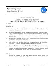
3 Measurement of Degradation Ratio of QZSS Receivers from ALOS-2 SAR System<br />
To confirm the degradation of QZSS LEX signal affected by ALOS-2 signals, JAXA had the<br />
compatibility test <strong>in</strong> 2011. Figure 4 shows the configuration of the compatibility test.<br />
The QZSS signal transmitted from the satellite was received at GPS antenna on the roof of the<br />
facility <strong>in</strong> Tsukuba Space Center, and mixed with the ALOS-2 signals generated by ALOS-2<br />
Eng<strong>in</strong>eer<strong>in</strong>g Models (EM) at the hybrid. The characteristics of ALOS-2 signals <strong>in</strong>cluded the<br />
pulse width, PRF, bandwidth, and the RF duty cycle were worst case <strong>in</strong> each observation modes<br />
of ALOS-2.<br />
The test case and results of the compatibility tests shows the Table 5. The SNR degradation<br />
typically ranges from -0.23 dB to -0.88 dB.<br />
FIGURE 4<br />
The configuration of compatibility test <strong>between</strong> QZSS receiver and ALOS-2<br />
outdoor<br />
<strong>in</strong>door<br />
QZSS real signal<br />
GPS ANT<br />
HYB<br />
QZSS<br />
Receiver<br />
Spectrum<br />
Anaryzer<br />
ALOS-2<br />
(SAR 4,5,6)<br />
Eng<strong>in</strong>eer<strong>in</strong>g Model<br />
PC<br />
3-July-2013 Page 20 of 21 <strong>REP</strong> <strong>SFCG</strong> <strong>32</strong>-<strong>2R1</strong>
TABLE 5<br />
Static Degradation measurements <strong>in</strong> QZSS/ALOS-2 compatibility demonstration test<br />
Demonstration test step configuration<br />
The level <strong>in</strong>to the QZSS receiver is the maximum level: -71.48<br />
dBW for the worst case test<br />
84 MHz bandwidth, PRF=1 960 Hz, Pulsewidth=51 µs<br />
Center frequency: 1257.5 MHz (SAR4)<br />
42 MHz bandwidth, PRF=1 477 Hz, Pulsewidth=46 µs<br />
Center frequency: 1257.5 MHz<br />
28 MHz bandwidth, PRF=2 637 Hz, Pulsewidth=25 µs<br />
Center frequency: 1257.5 MHz (SAR6)<br />
14 MHz bandwidth, PRF=1 915 Hz, Pulsewidth=36.6 µs<br />
Center frequency: 1257.5 MHz(SAR5)<br />
42 MHz bandwidth, PRF=2 900 Hz Pulsewidth=23.4 µs<br />
Center frequency: 1257.5 MHz<br />
28 MHz bandwidth, PRF=4 400 Hz, Pulsewidth=15 µs<br />
Center frequency: 1257.5 MHz(SAR6)<br />
14 MHz bandwidth, PRF=1 915 Hz Pulsewidth=36.6 µs<br />
Center frequency : 1236.5 MHz(SAR5)<br />
28 MHz bandwidth, PRF=2 637 Hz, Pulsewidth=25 µs<br />
Center frequency: 1278.5 MHz(SAR6)<br />
Lock/<br />
No lock<br />
LEX SNR<br />
change<br />
(dB)<br />
L2C SNR<br />
change<br />
(dB)<br />
Lock -0.88 -0.66<br />
Lock -0.72 -0.35<br />
Lock -0.58 -0.<strong>32</strong><br />
Lock -0.67 -0.<strong>32</strong><br />
Lock -0.60 -0.27<br />
Lock -0.47 -0.23<br />
Lock -0.34 -0.50<br />
Lock -0.65 -0.40<br />
4 Conclusion<br />
This document analyzes the shar<strong>in</strong>g <strong>between</strong> <strong>RNSS</strong> (GPS and QZSS) and <strong>EESS</strong> (active) <strong>in</strong> the<br />
<strong>1215</strong>-<strong>1300</strong> MHz band and presents results of compatibility measurements and possible<br />
compatibility measures <strong>between</strong> systems <strong>in</strong> the <strong>EESS</strong> (active) and systems <strong>in</strong> the <strong>RNSS</strong> <strong>in</strong> the<br />
band <strong>1215</strong>-<strong>1300</strong> MHz.<br />
The effect of pulsed RF <strong>in</strong>terference from the two spaceborne radars Scatterometer 2 and SAR3<br />
upon the two GPS receivers is a change <strong>in</strong> SNR or C/N 0 of less than 0.1 dB for Scatterometer 2<br />
and less than -1.4 dB for SAR3 for maximum RFI levels at the <strong>RNSS</strong> receivers. With mitigation<br />
measures, the SAR3 degradation to SNR can be reduced from -1.4 dB to -0.1 dB.<br />
For the QZSS receivers, the SNR degradation from ALOS-2 SAR typically ranges from -0.23 dB<br />
to -0.88 dB.<br />
3-July-2013 Page 21 of 21 <strong>REP</strong> <strong>SFCG</strong> <strong>32</strong>-<strong>2R1</strong>