Introduction to Finite Frame Theory - Frame Research Center
Introduction to Finite Frame Theory - Frame Research Center
Introduction to Finite Frame Theory - Frame Research Center

You also want an ePaper? Increase the reach of your titles
YUMPU automatically turns print PDFs into web optimized ePapers that Google loves.
<strong>Introduction</strong> <strong>to</strong> <strong>Finite</strong> <strong>Frame</strong> <strong>Theory</strong><br />
Peter G. Casazza, Gitta Kutyniok, and Friedrich Philipp<br />
1 Why <strong>Frame</strong>s?<br />
The Fourier transform has been a major <strong>to</strong>ol in analysis for over 100 years. However,<br />
it solely provides frequency information, and hides (in its phases) information<br />
concerning the moment of emission and duration of a signal. D. Gabor resolved<br />
this problem in 1946 [93] by introducing a fundamental new approach <strong>to</strong> signal<br />
decomposition. Gabor’s approach quickly became the paradigm for this area, because<br />
it provided resilience <strong>to</strong> additive noise, resilience <strong>to</strong> quantization, resilience<br />
<strong>to</strong> transmission losses as well as an ability <strong>to</strong> capture important signal characteristics.<br />
Unbeknownst <strong>to</strong> Gabor, he had discovered the fundamental properties of a<br />
frame without any of the formalism. In 1952, Duffin and Schaeffer [80] were working<br />
on some deep problems in non-harmonic Fourier series for which they required<br />
a formal structure for working with highly over-complete families of exponential<br />
functions in L 2 [0,1]. For this, they introduced the notion of a Hilbert space frame,<br />
for which Gabor’s approach is now a special case, falling in<strong>to</strong> the area of timefrequency<br />
analysis [98]. Much later – in the late 1980’s – the fundamental concept<br />
of frames was revived by Daubechies, Grossman and Mayer [77] (see also [76]),<br />
who showed its importance for data processing.<br />
Traditionally, frames were used in signal and image processing, non-harmonic<br />
Fourier series, data compression, and sampling theory. But <strong>to</strong>day, frame theory has<br />
ever increasing applications <strong>to</strong> problems in both pure and applied mathematics,<br />
Peter G. Casazza<br />
University of Missouri, Mathematics Department, Columbia, MO 65211, USA, e-mail: casazzap@missouri.edu<br />
Gitta Kutyniok<br />
Technische Universität Berlin, Department of Mathematics, 10623 Berlin, Germany, e-mail:<br />
kutyniok@math.tu-berlin.de<br />
Friedrich Philipp<br />
Technische Universität Berlin, Department of Mathematics, 10623 Berlin, Germany, e-mail:<br />
philipp@math.tu-berlin.de<br />
1
2 Peter G. Casazza, Gitta Kutyniok, and Friedrich Philipp<br />
physics, engineering, computer science, <strong>to</strong> name a few. Several of these applications<br />
will be investigated in this book. Since applications mainly require frames in finitedimensional<br />
spaces, this will be our focus. In this situation, a frame is a spanning<br />
set of vec<strong>to</strong>rs – which are generally redundant (over-complete) requiring control of<br />
its condition numbers. Thus a typical frame possesses more frame vec<strong>to</strong>rs than the<br />
dimension of the space, and each vec<strong>to</strong>r in the space will have infinitely many representations<br />
with respect <strong>to</strong> the frame. But it will also have one natural representation<br />
given by a special class of scalars called the frame coefficients of the vec<strong>to</strong>r. It is this<br />
redundancy of frames which is key <strong>to</strong> their significance for applications.<br />
The role of redundancy varies depending on the requirements of the applications<br />
at hand. First, redundancy gives greater design flexibility which allows frames <strong>to</strong> be<br />
constructed <strong>to</strong> fit a particular problem in a manner not possible by a set of linearly<br />
independent vec<strong>to</strong>rs. For instance, in areas such as quantum <strong>to</strong>mography, classes of<br />
orthonormal bases with the property that the modulus of the inner products of vec<strong>to</strong>rs<br />
from different bases are a constant are required. A second example comes from<br />
speech recognition, when a vec<strong>to</strong>r needs <strong>to</strong> be determined by the absolute value of<br />
the frame coefficients (up <strong>to</strong> a phase fac<strong>to</strong>r). A second major advantage of redundancy<br />
is robustness. By spreading the information over a wider range of vec<strong>to</strong>rs,<br />
resilience against losses (erasures) can be achieved, which are, for instance, a severe<br />
problem in wireless sensor networks for transmission losses or when sensors<br />
are intermittently fading out, modeling the brain where memory cells are dying out.<br />
A further advantage of spreading information over a wider range of vec<strong>to</strong>rs is <strong>to</strong><br />
mitigate the effects of noise in the signal.<br />
This represents a tiny fraction of the theory and applications of frame theory that<br />
you will encounter in this book. New theoretical insights and novel applications are<br />
continually arising due <strong>to</strong> the fact that the underlying principles of frame theory are<br />
basic ideas which are fundamental <strong>to</strong> a wide canon of areas of research. In this sense,<br />
frame theory might be regarded as partly belonging <strong>to</strong> applied harmonic analysis,<br />
functional analysis, opera<strong>to</strong>r theory as well as numerical linear algebra and matrix<br />
theory.<br />
1.1 The Role of Decompositions and Expansions<br />
Focussing on the finite-dimensional situation, let x be given data which we assume<br />
<strong>to</strong> belong <strong>to</strong> some real or complex N-dimensional Hilbert space H N . Further, let<br />
(ϕ i ) M i=1 be a representation system (i.e. a spanning set) in H N , which might be<br />
chosen from an existing catalogue, designed depending on the type of data we are<br />
facing, or learned from sample sets of the data.<br />
One common approach <strong>to</strong> data processing consists in the decomposition of the<br />
data x according <strong>to</strong> the system (ϕ i ) M i=1 by considering the map<br />
x ↦→ (〈x,ϕ i 〉) M i=1.
<strong>Introduction</strong> <strong>to</strong> <strong>Finite</strong> <strong>Frame</strong> <strong>Theory</strong> 3<br />
As we will see, the generated sequence (〈x,ϕ i 〉) M i=1 belonging <strong>to</strong> l 2({1,...,M}) can<br />
then be used, for instance, for transmission of x. Also, careful choice of the representation<br />
system enables us <strong>to</strong> solve a variety of analysis tasks. As an example,<br />
under certain conditions the positions and orientations of edges of an image x are<br />
determined by those indices i ∈ {1,...,M} belonging <strong>to</strong> the largest coefficients in<br />
magnitude |〈x,ϕ i 〉|, i.e., by hard thresholding, in the case that (ϕ i ) M i=1 is a shearlet<br />
system (see [116]). Finally, the sequence (〈x,ϕ i 〉) M i=1 allows compression of x,<br />
which is in fact the heart of the new JPEG2000 compression standard when choosing<br />
(ϕ i ) M i=1 <strong>to</strong> be a wavelet system [141].<br />
An accompanying approach is the expansion of the data x by considering sequences<br />
(c i ) M i=1 satisfying x =<br />
M<br />
∑<br />
i=1<br />
c i ϕ i .<br />
It is well known that suitably chosen representation systems allow sparse sequences<br />
(c i ) M i=1 in the sense that ‖c‖ 0 = #{i : c i ≠ 0} is small. For example, certain wavelet<br />
systems typically sparsify natural images in this sense (see for example [78, 123,<br />
134] and the references therein). This observation is key <strong>to</strong> allowing the application<br />
of the abundance of existing sparsity methodologies such as Compressed Sensing<br />
[87] <strong>to</strong> x. In contrast <strong>to</strong> this viewpoint which assumes x as explicitly given, the<br />
approach of expanding the data is also highly beneficial in the case where x is only<br />
implicitly given, which is, for instance, the problem all PDE solvers face. Hence,<br />
using (ϕ i ) M i=1 as a generating system for the trial space, the PDE solvers task reduces<br />
<strong>to</strong> computing (c i ) M i=1 which is advantageous for deriving efficient solvers provided<br />
that – as before – a sparse sequence does exist (see, e.g., [107, 74]).<br />
1.2 Beyond Orthonormal Bases<br />
To choose the representation system (ϕ i ) N i=1<br />
<strong>to</strong> form an orthonormal basis for H<br />
N<br />
is the standard choice. However, the linear independence of such a system causes a<br />
variety of problems for the aforementioned applications.<br />
Starting with the decomposition viewpoint, using (〈x,ϕ i 〉) N i=1<br />
for transmission<br />
is far from being robust <strong>to</strong> erasures, since the erasure of only a single coefficient<br />
causes a true information loss. Also, for analysis tasks orthonormal bases are far<br />
from being advantageous, since they do not allow any flexibility in design, which is<br />
for instance needed for the design of directional representation systems. In fact, it is<br />
conceivable that no orthonormal basis with paralleling properties such as curvelets<br />
or shearlets does exist. A task benefitting from linear independence is compression,<br />
which naturally requires a minimal number of coefficients.<br />
Also, from an expansion point of view, the utilization of orthonormal bases is<br />
not advisable. A particular problem affecting sparsity methodologies as well as the<br />
utilization for PDE solvers is the uniqueness of the sequence (c i ) M i=1 . This nonflexibility<br />
prohibits the search for a sparse coefficient sequence.
4 Peter G. Casazza, Gitta Kutyniok, and Friedrich Philipp<br />
It is evident that those problems can be tackled by allowing the system (ϕ i ) M i=1 <strong>to</strong><br />
be redundant. Certainly, numerical stability issues in the typical processing of data<br />
x ↦→ (〈x,ϕ i 〉) M i=1 ↦→<br />
M<br />
∑<br />
i=1<br />
〈x,ϕ i 〉 ˜ϕ i ≈ x<br />
with an adapted system ( ˜ϕ i ) M i=1 have <strong>to</strong> be taken in<strong>to</strong> account. This leads naturally<br />
<strong>to</strong> the notion of a (Hilbert space) frame. The main idea is <strong>to</strong> have a controlled norm<br />
equivalence between the data x and the sequence of coefficients (〈x,ϕ i 〉) M i=1 .<br />
The area of frame theory has very close relations <strong>to</strong> other research fields in both<br />
pure and applied mathematics. General (Hilbert space) frame theory – in particular,<br />
including the infinite-dimensional situation – intersects functional analysis and<br />
opera<strong>to</strong>r theory. It also bears close relations <strong>to</strong> the novel area of applied harmonic<br />
analysis, in which the design of representation systems – typically by a careful partitioning<br />
of the Fourier domain – is one major objective. Some researchers even consider<br />
frame theory as belonging <strong>to</strong> this area. Restricting <strong>to</strong> the finite-dimensional<br />
situation – in which cus<strong>to</strong>marily the term finite frame theory is used – the classical<br />
areas of matrix theory and numerical linear algebra have close intersections, but<br />
also, for instance, the novel area of Compressed Sensing as already pointed out.<br />
Nowadays, frames have established themselves as a standard notion in applied<br />
mathematics, computer science, and engineering. <strong>Finite</strong> frame theory deserves special<br />
attention due <strong>to</strong> its importance for applications, and might be even considered a<br />
research area of its own. This is also the reason why this book specifically focusses<br />
on finite frame theory. The subsequent chapters will show the diversity of this rich<br />
and vivid research area <strong>to</strong> date ranging from the development of frameworks <strong>to</strong> analyze<br />
specific properties of frames, the design of different classes of frames <strong>to</strong> various<br />
applications of frames and also extensions of the notion of a frame.<br />
1.3 Outline<br />
In the sequel, in Section 2 we first provide some background information on Hilbert<br />
space theory and opera<strong>to</strong>r theory <strong>to</strong> make this book self-contained. <strong>Frame</strong>s are then<br />
subsequently introduced in Section 3, followed by a discussion of the four main<br />
opera<strong>to</strong>rs associated with a frame, namely the analysis, synthesis, frame, and Grammian<br />
opera<strong>to</strong>r (see Section 4). Reconstruction results and algorithms naturally including<br />
the notion of a dual frame is the focus of Section 5. This is followed by the<br />
presentation of different constructions of tight as well as non-tight frames (Section<br />
6), and a discussion of some crucial properties of frames, in particular, their spanning<br />
properties, the redundancy of a frame, and equivalence relations among frames<br />
in Section 7. This chapter is concluded by brief introductions <strong>to</strong> diverse applications<br />
and extensions of frames (Sections 8 and 9).
<strong>Introduction</strong> <strong>to</strong> <strong>Finite</strong> <strong>Frame</strong> <strong>Theory</strong> 5<br />
2 Background Material<br />
Let us start by recalling some basic definitions and results from Hilbert space theory<br />
and opera<strong>to</strong>r theory, which will be required for all subsequent chapters. We do not<br />
include the proofs of the presented results, and refer <strong>to</strong> the standard literature such<br />
as, for instance, [153] for Hilbert space theory and [71, 105, 130] for opera<strong>to</strong>r theory.<br />
We would like <strong>to</strong> emphasize that all following results are solely stated in the finite<br />
dimensional setting, which is the focus of this book.<br />
2.1 Review of Basics from Hilbert Space <strong>Theory</strong><br />
Letting N be a positive integer, we denote by H N a real or complex N-dimensional<br />
Hilbert space. This will be the space considered throughout this book. Sometimes,<br />
if it is convenient, we identify H N with R N or C N . By 〈·,·〉 and ‖ · ‖ we denote the<br />
inner product on H N and its corresponding norm, respectively.<br />
Let us now start with the origin of frame theory, which is the notion of an orthonormal<br />
basis. Alongside, we recall the basic definitions we will also require in<br />
the sequel.<br />
Definition 1. A vec<strong>to</strong>r x ∈ H N is called normalized if ‖x‖ = 1. Two vec<strong>to</strong>rs x,y ∈<br />
H N are called orthogonal if 〈x,y〉 = 0. A system (e i ) k i=1 of vec<strong>to</strong>rs in H N is called<br />
(a) complete (or a spanning set) if span{e i } k i=1 = H N .<br />
(b) orthogonal if for all i ≠ j, the vec<strong>to</strong>rs e i and e j are orthogonal.<br />
(c) orthonormal if it is orthogonal and each e i is normalized.<br />
(e) orthonormal basis for H N if it is complete and orthonormal.<br />
A fundamental result in Hilbert space theory is Parseval’s Identity.<br />
Proposition 1 (Parseval’s Identity). If (e i ) N i=1 is an orthonormal basis for H N ,<br />
then, for every x ∈ H N , we have<br />
‖x‖ 2 =<br />
N<br />
∑<br />
i=1<br />
|〈x,e i 〉| 2 .<br />
Interpreting this identity from a signal processing point of view, it implies that the<br />
energy of the signal is preserved under the map x ↦→ (〈x,e i 〉) N i=1<br />
which we will later<br />
refer <strong>to</strong> as the analysis map. We would also like <strong>to</strong> mention at this point, that this<br />
identity is not only satisfied by orthonormal bases. In fact, redundant systems (“nonbases”)<br />
such as (e 1 , √ 1<br />
2<br />
e 2 , √ 1<br />
2<br />
e 2 , √ 1 3<br />
e 3 , √ 1<br />
3<br />
e 3 , √ 1 1<br />
3<br />
e 3 ,..., √ 1<br />
N<br />
e N ,..., √<br />
N<br />
e N ) also satisfy<br />
this inequality, and will later be coined Parseval frames.<br />
Parseval’s identity has the following implication, which shows that a vec<strong>to</strong>r x can<br />
be recovered from the coefficients (〈x,e i 〉) N i=1<br />
by a simple procedure. Thus, from<br />
an application point of view, this result can also be interpreted as a reconstruction<br />
formula.
6 Peter G. Casazza, Gitta Kutyniok, and Friedrich Philipp<br />
Corollary 1. If (e i ) N i=1 is an orthonormal basis for H N , then, for every x ∈ H N ,<br />
we have<br />
x =<br />
N<br />
∑<br />
i=1<br />
〈x,e i 〉e i .<br />
Next, we present a series of identities and inequalities, which are basics exploited<br />
in various proofs.<br />
Proposition 2. Let x, ˜x ∈ H N .<br />
(i) Cauchy-Schwartz Inequality. We have<br />
|〈x, ˜x〉| ≤ ‖x‖‖ ˜x‖,<br />
with equality if and only if x = c ˜x for some constant c.<br />
(ii) Triangle Inequality. We have<br />
‖x + ˜x‖ ≤ ‖x‖ + ‖ ˜x‖.<br />
(iii) Polarization Identity (Real Form). If H N is real, then<br />
〈x, ˜x〉 = 1 4<br />
[<br />
‖x + ˜x‖ 2 − ‖x − ˜x‖ 2] .<br />
(iv) Polarization Identity (Complex Form). If H N is complex, then<br />
〈x, ˜x〉 = 1 4<br />
[<br />
‖x + ˜x‖ 2 − ‖x − ˜x‖ 2] + i 4<br />
[<br />
‖x + i ˜x‖ 2 − ‖x − i ˜x‖ 2] .<br />
(v) Pythagorean Theorem. Given pairwise orthogonal vec<strong>to</strong>rs (x i ) M i=1 ∈ H N , we<br />
have ∥ ∥ ∥∥∥∥ M ∥∥∥∥<br />
2<br />
M<br />
∑ x i = ∑ ‖x i ‖ 2 .<br />
i=1 i=1<br />
We next turn <strong>to</strong> considering subspaces in H N , again starting with the basic notations<br />
and definitions.<br />
Definition 2. Let W ,V be subspaces of H N .<br />
(a) A vec<strong>to</strong>r x ∈ H N is called orthogonal <strong>to</strong> W (denoted by x ⊥ W ), if<br />
〈x, ˜x〉 = 0 for all ˜x ∈ W .<br />
The orthogonal complement of W is then defined by<br />
W ⊥ = {x ∈ H N : x ⊥ W }.<br />
(b) The subspaces W and V are called orthogonal subspaces (denoted by W ⊥ V ),<br />
if W ⊂ V ⊥ (or, equivalently, V ⊂ W ⊥ ).
<strong>Introduction</strong> <strong>to</strong> <strong>Finite</strong> <strong>Frame</strong> <strong>Theory</strong> 7<br />
The notion of orthogonal direct sums, which will play an essential role in Chapter<br />
[166], can be regarded as a generalization of Parseval’s identity (Proposition 1).<br />
Definition 3. Let (W i ) M i=1 be a family of subspaces of H N . Then their orthogonal<br />
direct sum is defined as the space<br />
( M∑<br />
i=1⊕W i<br />
)<br />
with inner product defined by<br />
〈x, ˜x〉 =<br />
M<br />
∑<br />
i=1<br />
l 2 := W 1 × ... × W M<br />
〈x i , ˜x i 〉 for all x = (x i ) M i=1, ˜x = ( ˜x i ) M i=1 ∈<br />
( M∑<br />
i=1⊕W i<br />
)<br />
The extension of Parseval’s identity can be seen when choosing ˜x = x yielding<br />
‖x‖ 2 = ∑ M i=1 ‖x i‖ 2 .<br />
l 2 .<br />
2.2 Review of Basics from Opera<strong>to</strong>r <strong>Theory</strong><br />
We next introduce the basic results from opera<strong>to</strong>r theory used throughout this book.<br />
We first recall that each opera<strong>to</strong>r has an associated matrix representation.<br />
Definition 4. Let T : H N → H K be a linear opera<strong>to</strong>r, let (e i ) N i=1<br />
be an orthonormal<br />
basis for H N , and let (g i ) K i=1 be an orthonormal basis for H K . Then the matrix<br />
representation of T (with respect <strong>to</strong> the orthonormal bases (e i ) N i=1 and (g i) K i=1 ) is a<br />
matrix of size K × N and is given by A = (a i j ) K , N<br />
i=1, j=1 , where<br />
a i j = 〈Te j ,g i 〉.<br />
For all x ∈ H N with c = (〈x,e i 〉) N i=1<br />
we have<br />
T x = Ac.<br />
2.2.1 Invertibility<br />
We start with the following definition.<br />
Definition 5. Let T : H N → H K be a linear opera<strong>to</strong>r.<br />
(a) The kernel of T is defined by kerT := {x ∈ H N : T x = 0}. Its range is ranT :=<br />
{T x : x ∈ H N }, sometimes also called image and denoted by imT . The rank of<br />
T , rankT , is the dimension of the range of T .
8 Peter G. Casazza, Gitta Kutyniok, and Friedrich Philipp<br />
(b) The opera<strong>to</strong>r T is called injective (or one-<strong>to</strong>-one), if kerT = {0}, and surjective<br />
(or on<strong>to</strong>), if ranT = H K . It is called bijective (or invertible), if T is both injective<br />
and surjective.<br />
(c) The adjoint opera<strong>to</strong>r T ∗ : H K → H N is defined by<br />
(d) The norm of T is defined by<br />
〈T x, ˜x〉 = 〈x,T ∗ ˜x〉 for all x ∈ H N and ˜x ∈ H K .<br />
‖T ‖ := sup{‖T x‖ : ‖x‖ = 1}.<br />
The next result states several relations between these notions.<br />
Proposition 3. (i) Let T : H N → H K be a linear opera<strong>to</strong>r. Then<br />
dimH N = N = dimkerT + rankT.<br />
Moreover, if T is injective, then T ∗ T is also injective.<br />
(ii) Let T : H N → H N be a linear opera<strong>to</strong>r. Then T is injective if and only if it is<br />
surjective. Moreover , kerT = (ranT ∗ ) ⊥ , and hence<br />
H N = kerT ⊕ ranT ∗ .<br />
If T : H N → H N is an injective opera<strong>to</strong>r, then T is obviously invertible. If an<br />
opera<strong>to</strong>r T : H N → H K is not injective, we can make T injective by restricting it <strong>to</strong><br />
(kerT ) ⊥ . However, T | (kerT ) ⊥ might still not be invertible, since it does not need <strong>to</strong><br />
be surjective. This can be ensured by considering the opera<strong>to</strong>r T : (kerT ) ⊥ → ranT ,<br />
which is now invertible.<br />
The Moore-Penrose inverse of an injective opera<strong>to</strong>r provides a one-sided inverse<br />
for the opera<strong>to</strong>r.<br />
Definition 6. Let T : H N → H K be an injective, linear opera<strong>to</strong>r. The Moore-<br />
Penrose inverse of T , T † , is defined by<br />
T † = (T ∗ T ) −1 T ∗ .<br />
It is immediate <strong>to</strong> prove invertibility from the left as stated in the following result.<br />
Proposition 4. If T : H N → H K is an injective, linear opera<strong>to</strong>r, then T † T = Id.<br />
Thus, T † plays the role of the inverse on ranT – not on all of H K . It projects a<br />
vec<strong>to</strong>r from H K on<strong>to</strong> ranT and then inverts the opera<strong>to</strong>r on this subspace.<br />
A more general notion of this inverse is called the pseudo-inverse, which can be<br />
applied <strong>to</strong> a non-injective opera<strong>to</strong>r. It, in fact, adds one more step <strong>to</strong> the action of<br />
T † by first restricting <strong>to</strong> (kerT ) ⊥ <strong>to</strong> enforce injectivity of the opera<strong>to</strong>r followed<br />
by application of the Moore-Penrose inverse of this new opera<strong>to</strong>r. This pseudoinverse<br />
can be derived from the singular value decomposition. Recalling that by<br />
fixing orthonormal bases of the domain and range of a linear opera<strong>to</strong>r we derive an
<strong>Introduction</strong> <strong>to</strong> <strong>Finite</strong> <strong>Frame</strong> <strong>Theory</strong> 9<br />
associated unique matrix representation, we begin by stating this decomposition in<br />
terms of a matrix.<br />
Theorem 1. Let A be an M × N matrix. Then there exist an M × M unitary matrix<br />
U (see Definition 9), an N × N unitary matrix V , and an M × N diagonal matrix Σ<br />
with nonnegative, decreasing real entries on the diagonal such that<br />
A = UΣV ∗ .<br />
Hereby, an M × N diagonal matrix with M ≠ N is an M × N matrix (a i j ) M , N<br />
i=1, j=1<br />
with a i j = 0 for i ≠ j.<br />
Definition 7. Let A be an M ×N matrix, and let U,Σ, and V be chosen as in Theorem<br />
1. Then A = UΣV ∗ is called the singular value decomposition (SVD) of A. The<br />
column vec<strong>to</strong>rs of U are called the left singular vec<strong>to</strong>rs, and the column vec<strong>to</strong>rs of<br />
V are referred <strong>to</strong> as the right singular vec<strong>to</strong>rs of A.<br />
The pseudo-inverse A + of A can be deduced from the SVD in the following way.<br />
Theorem 2. Let A be an M × N matrix, and let A = UΣV ∗ be its singular value<br />
decomposition. Then<br />
A + = V Σ + U ∗ ,<br />
where Σ + is the N × M diagonal matrix arising from Σ ∗ by inverting the non-zero<br />
(diagonal) entries.<br />
2.2.2 Riesz Bases<br />
In the previous subsection, we already recalled the notion of an orthonormal basis.<br />
However, sometimes the requirement of orthonormality is <strong>to</strong>o strong, but uniqueness<br />
of a decomposition as well as stability shall be retained. The notion of a Riesz basis,<br />
which we next introduce, satisfies these desiderata.<br />
Definition 8. A family of vec<strong>to</strong>rs (ϕ i ) N i=1 in a Hilbert space H N is a Riesz basis<br />
with lower (respectively, upper) Riesz bounds A (resp. B), if, for all scalars (a i ) N i=1 ,<br />
we have<br />
∥<br />
N<br />
A∑<br />
|a i | 2 N ∥∥∥∥<br />
2<br />
N<br />
≤<br />
∥∑<br />
a i ϕ i ≤ B∑<br />
|a i | 2 .<br />
i=1<br />
i=1<br />
i=1<br />
The following result is immediate from the definition.<br />
Proposition 5. Let (ϕ i ) N i=1<br />
be a family of vec<strong>to</strong>rs. Then the following conditions are<br />
equivalent.<br />
(i) (ϕ i ) N i=1 is a Riesz basis for H N with Riesz bounds A and B.<br />
(ii) For any orthonormal basis (e i ) N i=1 for H N , the opera<strong>to</strong>r T on H N given by<br />
Te i = ϕ i for all i = 1,2,...,N is an invertible opera<strong>to</strong>r with ‖T ‖ 2 ≤ B and<br />
‖T −1 ‖ −2 ≥ A.
10 Peter G. Casazza, Gitta Kutyniok, and Friedrich Philipp<br />
2.2.3 Diagonalization<br />
Next, we continue our list of important properties of linear opera<strong>to</strong>rs.<br />
Definition 9. A linear opera<strong>to</strong>r T : H N → H K is called<br />
(a) self-adjoint, if H N = H K and T = T ∗ .<br />
(b) normal, if T ∗ T = T T ∗ .<br />
(c) an isometry, if ‖T x‖ = ‖x‖ for all x ∈ H N .<br />
(d) a co-isometry, if T ∗ is an isometry.<br />
(e) positive, if H N = H K , T is self-adjoint, and 〈T x,x〉 ≥ 0 for all x ∈ H N .<br />
(f) unitary, if it is a surjective isometry.<br />
From the variety of basic relations and results of those notions, the next proposition<br />
presents a selection of those which will be required in the sequel.<br />
Proposition 6. Let T : H N → H K be a linear opera<strong>to</strong>r.<br />
(i) We have ‖T ∗ T ‖ = ‖T ‖ 2 , and T ∗ T and T T ∗ are self-adjoint.<br />
(ii) If N = K, the following conditions are equivalent.<br />
(1) T is self-adjoint.<br />
(2) 〈T x, ˜x〉 = 〈x,T ˜x〉 for all x, ˜x ∈ H N .<br />
(3) If H N is complex, 〈T x,x〉 ∈ R for all x ∈ H N .<br />
(iii) The following conditions are equivalent.<br />
(1) T is an isometry.<br />
(2) T ∗ T = Id.<br />
(3) 〈T x,T ˜x〉 = 〈x, ˜x〉 for all x, ˜x ∈ H N .<br />
(iv) The following conditions are equivalent.<br />
(1) T is unitary.<br />
(2) T and T ∗ are isometric.<br />
(3) T T ∗ = Id and T ∗ T = Id.<br />
(v) If U is a unitary opera<strong>to</strong>r, then ‖UT ‖ = ‖T ‖ = ‖TU‖.<br />
Diagonalizations of opera<strong>to</strong>rs are frequently utilized <strong>to</strong> derive an understanding<br />
of the action of an opera<strong>to</strong>r. The following definitions lay the groundwork for this<br />
theory.<br />
Definition 10. Let T : H N → H N be a linear opera<strong>to</strong>r. A non-zero vec<strong>to</strong>r x ∈ H N<br />
is an eigenvec<strong>to</strong>r of T with eigenvalue λ, if T x = λx. The opera<strong>to</strong>r T is called<br />
orthogonally diagonalizable, if there exists an orthonormal basis (e i ) N i=1 of H N<br />
consisting of eigenvec<strong>to</strong>rs of T .<br />
We start with an easy observation.<br />
Proposition 7. For any linear opera<strong>to</strong>r T : H N → H K , the non-zero eigenvalues<br />
of T ∗ T and T T ∗ are the same.
<strong>Introduction</strong> <strong>to</strong> <strong>Finite</strong> <strong>Frame</strong> <strong>Theory</strong> 11<br />
If the opera<strong>to</strong>r is unitary, self-adjoint or positive, we have more information on<br />
the eigenvalues stated in the next result, which follows immediately from Proposition<br />
6.<br />
Corollary 2. Let T : H N → H N be a linear opera<strong>to</strong>r.<br />
(i) If T is unitary, then its eigenvalues have modulus one.<br />
(ii) If T is self-adjoint, then its eigenvalues are real.<br />
(iii) If T is positive, then its eigenvalues are non-negative.<br />
This fact allows us <strong>to</strong> introduce a condition number associated with each invertible<br />
positive opera<strong>to</strong>r.<br />
Definition 11. Let T : H N → H N be an invertible positive opera<strong>to</strong>r with eigenvalues<br />
λ 1 ≥ λ 2 ≥ ... ≥ λ N . Then its condition number is defined by λ 1<br />
λ N<br />
.<br />
We next state a fundamental result in opera<strong>to</strong>r theory which has its analogue in<br />
the infinite-dimensional setting called the spectral theorem.<br />
Theorem 3. Let H N be complex and let T : H N → H N be a linear opera<strong>to</strong>r. Then<br />
the following conditions are equivalent.<br />
(i) T is normal.<br />
(ii) T is orthogonally diagonizable.<br />
(iii) There exists a diagonal matrix representation of T .<br />
(iv) There exist an orthonormal basis (e i ) N i=1 of H N and values λ 1 ,...,λ N such that<br />
Moreover,<br />
T x =<br />
N<br />
∑<br />
i=1<br />
λ i 〈x,e i 〉e i for all x ∈ H N .<br />
‖T ‖ 2 = max<br />
1≤i≤N λ i.<br />
Since every self-adjoint opera<strong>to</strong>r is normal we obtain the following corollary<br />
(which is independent of whether H N is real or complex).<br />
Corollary 3. A self-adjoint opera<strong>to</strong>r is orthogonally diagonalizable.<br />
Another consequence of Theorem 3 is the following result, which in particular<br />
allows the definition of the n-th root of a positive opera<strong>to</strong>r.<br />
Corollary 4. Let T : H N → H N be an invertible positive opera<strong>to</strong>r with normalized<br />
eigenvec<strong>to</strong>rs (e i ) N i=1 and respective eigenvalues (λ i) N i=1<br />
, let a ∈ R, and define an<br />
opera<strong>to</strong>r T a : H N → H N by<br />
T a x =<br />
N<br />
∑<br />
i=1<br />
λ a<br />
i 〈x,e i 〉e i for all x ∈ H N .<br />
Then T a is a positive opera<strong>to</strong>r and T a T b = T a+b for a,b ∈ R. In particular, T −1<br />
and T −1/2 are positive opera<strong>to</strong>rs.
12 Peter G. Casazza, Gitta Kutyniok, and Friedrich Philipp<br />
Finally, we define the trace of an opera<strong>to</strong>r, which, by using Theorem 3, can be<br />
expressed in terms of eigenvalues.<br />
Definition 12. Let T : H N → H N be an opera<strong>to</strong>r. Then, the trace of T is defined<br />
by<br />
TrT =<br />
N<br />
∑<br />
i=1<br />
where (e i ) N i=1 is an arbitrary orthonormal basis for H N .<br />
〈Te i ,e i 〉, (1)<br />
The trace is well defined since the sum in Equation 1 is independent of the choice<br />
of the orthonormal basis.<br />
Corollary 5. Let T : H N → H N be an orthogonally diagonalizable opera<strong>to</strong>r, and<br />
let (λ i ) N i=1 be its eigenvalues. Then TrT =<br />
N<br />
∑<br />
i=1<br />
λ i .<br />
2.2.4 Projection Opera<strong>to</strong>rs<br />
Subspaces are closely intertwined with associated projection opera<strong>to</strong>rs which map<br />
vec<strong>to</strong>rs on<strong>to</strong> the subspace either orthogonally or not. Although orthogonal projections<br />
are more often used, in Chapter [166] we will require the more general notion.<br />
Definition 13. Let P : H N → H N be a linear opera<strong>to</strong>r. Then P is called a projection,<br />
if P 2 = P. This projection is called orthogonal, if P is in addition self-adjoint.<br />
For the sake of brevity, orthogonal projections are often simply referred <strong>to</strong> as<br />
projections provided there is no danger of misinterpretation.<br />
Relating <strong>to</strong> our previous comment, for any subspace W of H N , there exists<br />
a unique orthogonal projection P of H N having W as its range. This projection<br />
can be constructed as follows: Let m denote the dimension of W , and choose an<br />
orthonormal basis (e i ) m i=1 of W . Then, for any x ∈ H N , we set<br />
Px =<br />
m<br />
∑<br />
i=1<br />
〈x,e i 〉e i .<br />
It is important <strong>to</strong> notice that also Id − P is an orthogonal projection of H N , this<br />
time on<strong>to</strong> the subspace W ⊥ .<br />
An orthogonal projection P has the crucial property that each given vec<strong>to</strong>r of<br />
H N is mapped <strong>to</strong> the closest vec<strong>to</strong>r in the range of P.<br />
Lemma 1. Let W be a subspace of H N , let P be the orthogonal projection on<strong>to</strong><br />
W , and let x ∈ H N . Then
<strong>Introduction</strong> <strong>to</strong> <strong>Finite</strong> <strong>Frame</strong> <strong>Theory</strong> 13<br />
‖x − Px‖ ≤ ‖x − ˜x‖ for all ˜x ∈ W .<br />
Moreover, if ‖x − Px‖ = ‖x − ˜x‖ for some ˜x ∈ W , then ˜x = Px.<br />
The next result gives the relationship between trace and rank for projections. This<br />
follows from the definition of an orthogonal projection and Corollaries 3 and 5.<br />
Proposition 8. Let P be the orthogonal projection on<strong>to</strong> a subspace W of H N , and<br />
let m = dimW . Then P is orthogonally diagonalizable with eigenvalue 1 of multiplicity<br />
m and eigenvalue 0 of multiplicity N −m. In particular, we have that TrP = m.<br />
3 Basics of <strong>Finite</strong> <strong>Frame</strong> <strong>Theory</strong><br />
We start by presenting the basics of finite frame theory. For illustration purposes,<br />
we then present some exemplary frame classes. At this point, we would also like <strong>to</strong><br />
refer <strong>to</strong> the monographs and books [35, 36, 100, 101, 112] as well as <strong>to</strong> [66, 67] for<br />
infinite-dimensional frame theory.<br />
3.1 Definition of a <strong>Frame</strong><br />
The definition of a (Hilbert space) frame originates from early work by Duffin and<br />
Schaeffer [80] on nonharmonic Fourier series. The main idea, as already discussed<br />
in Section 1, is <strong>to</strong> weaken Parseval’s identity yet <strong>to</strong> still retain norm equivalence<br />
between a signal and its frame coefficients.<br />
Definition 14. A family of vec<strong>to</strong>rs (ϕ i ) M i=1 in H N is called a frame for H N , if there<br />
exist constants 0 < A ≤ B < ∞ such that<br />
A‖x‖ 2 ≤<br />
M<br />
∑<br />
i=1<br />
The following notions are related <strong>to</strong> a frame (ϕ i ) M i=1 .<br />
|〈x,ϕ i 〉| 2 ≤ B‖x‖ 2 for all x ∈ H N . (2)<br />
(a) The constants A and B as in (2) are called lower and upper frame bound for the<br />
frame, respectively. The largest lower frame bound and the smallest upper frame<br />
bound are denoted by A op ,B op and are called the optimal frame bounds.<br />
(b) Any family (ϕ i ) M i=1 satisfying the right hand side inequality in (2) is called a<br />
B-Bessel sequence.<br />
(c) If A = B is possible in (2), then (ϕ i ) M i=1 is called an A-tight frame.<br />
(d) If A = B = 1 is possible in (2) – i.e., Parseval’s Identity holds –, then (ϕ i ) M i=1 is<br />
called a Parseval frame.<br />
(e) If there exists a constant c such that ‖ϕ i ‖ = c for all i = 1,2,...,M, then (ϕ i ) M i=1<br />
is an equal-norm frame. If c = 1, (ϕ i ) M i=1 is a unit-norm frame.
14 Peter G. Casazza, Gitta Kutyniok, and Friedrich Philipp<br />
(f) If there exists a constant c such that |〈ϕ i ,ϕ j 〉| = c for all i ≠ j, then (ϕ i ) M i=1 is<br />
called an equi-angular frame.<br />
(g) The values (〈x,ϕ i 〉) M i=1 are called the frame coefficients of the vec<strong>to</strong>r x with respect<br />
<strong>to</strong> the frame (ϕ i ) M i=1 .<br />
(h) The frame (ϕ i ) M i=1 is called exact, if (ϕ i) i∈I ceases <strong>to</strong> be a frame for H N for every<br />
I = {1,...,M} \ {i 0 }, i 0 ∈ {1,...,M}.<br />
We can immediately make the following useful observations.<br />
Lemma 2. Let (ϕ i ) M i=1 be a family of vec<strong>to</strong>rs in H N .<br />
(i) If (ϕ i ) M i=1 is an orthonormal basis, then (ϕ i) M i=1 is a Parseval frame. The converse<br />
is not true in general.<br />
(ii) (ϕ i ) M i=1 is a frame for H N if and only if it is a spanning set for H N .<br />
(iii) (ϕ i ) M i=1 is a unit-norm Parseval frame if and only if it is an orthonormal basis.<br />
(iv) If (ϕ i ) M i=1 is an exact frame for H N , then it is a basis of H N , i.e. a linearly<br />
independent spanning set.<br />
Proof. (i). The first part is an immediate consequence of Proposition 1. For the second<br />
part, let (e i ) N i=1 and (g i) N i=1 be orthonormal bases for H N . Then (e i / √ 2) N i=1 ∪<br />
(g i / √ 2) N i=1 is a Parseval frame for H N , but not an orthonormal basis.<br />
(ii). If (ϕ i ) M i=1 is not a spanning set for H N then there exists x ≠ 0 such that<br />
〈x,ϕ i 〉 = 0 for all i = 1,...,M. Hence, (ϕ i ) M i=1 cannot be a frame. Conversely, assume<br />
that (ϕ i ) M i=1 is not a frame. Then there exists a sequence (x n) ∞ n=1 of normalized<br />
vec<strong>to</strong>rs in H N such that ∑ M i=1 |〈x n,ϕ i 〉| 2 < 1/n for all n ∈ N. Hence, the limit x of<br />
a convergent subsequence of (x n ) ∞ n=1 satisfies 〈x,ϕ i〉 = 0 for all i = 1,...,M. Since<br />
‖x‖ = 1, it follows that (ϕ i ) M i=1 is not a spanning set.<br />
(iii). By the Parseval property, for each i 0 ∈ {1,...,M}, we have<br />
‖ϕ i0 ‖ 2 2 =<br />
M<br />
∑<br />
i=1<br />
M<br />
∑<br />
|〈ϕ i0 ,ϕ i 〉| 2 = ‖ϕ i0 ‖ 4 2 + |〈ϕ i0 ,ϕ i 〉| 2 .<br />
i=1,i≠i 0<br />
Since the frame vec<strong>to</strong>rs are normalized, we conclude that<br />
M<br />
∑<br />
i=1,i≠i 0<br />
|〈ϕ i0 ,ϕ i 〉| 2 = 0<br />
for all i 0 ∈ {1,...,M}.<br />
Hence 〈ϕ i ,ϕ j 〉 = 0 for all i ≠ j. Thus, (ϕ i ) M i=1 is an orthonormal system which is<br />
complete by (ii), and (iii) is proved.<br />
(iv). If (ϕ i ) M i=1 is a frame, by (ii), it is also a spanning set for H N . Towards<br />
a contradiction, assume that (ϕ i ) M i=1 is linearly dependent. Then there exist some<br />
i 0 ∈ {1,...,M} and values λ i , i ∈ I := {1,...,M} \ {i 0 } such that<br />
ϕ i0 = ∑λ i ϕ i .<br />
i∈I<br />
This implies that (ϕ i ) i∈I is also a frame, thus contradicting exactness of the frame.<br />
⊓⊔
<strong>Introduction</strong> <strong>to</strong> <strong>Finite</strong> <strong>Frame</strong> <strong>Theory</strong> 15<br />
Before presenting some insightful basic results in frame theory, we now first<br />
discuss some examples of frames <strong>to</strong> build up intuition.<br />
3.2 Examples<br />
By Lemma 2 (iii), orthonormal bases are unit-norm Parseval frames (and vice versa).<br />
However, applications typically require redundant Parseval frames. One basic way<br />
<strong>to</strong> approach this construction problem is <strong>to</strong> build redundant Parseval frames using<br />
orthonormal bases, and we will present several examples in the sequel. Since the<br />
associated proofs are straightforward, we leave them <strong>to</strong> the interested reader.<br />
Example 1. Let (e i ) N i=1 be an orthonormal basis for H N .<br />
(1) The system<br />
(e 1 ,0,e 2 ,0,...,e N ,0)<br />
is a Parseval frame for H N . This example indicates that a Parseval frame can<br />
indeed contain zero vec<strong>to</strong>rs.<br />
(2) The system<br />
(<br />
e 1 , e 2<br />
√ , e 2<br />
√ , e 3<br />
√ , e 3<br />
√ , e 3<br />
√ ,..., e N<br />
√ ,..., e N<br />
√<br />
),<br />
2 2 3 3 3 N N<br />
is a Parseval frame for H N . This example indicates two important issues: Firstly,<br />
a Parseval frame can have multiple copies of a single vec<strong>to</strong>r. Secondly, the norms<br />
of vec<strong>to</strong>rs of an (infinite) Parseval frame can converge <strong>to</strong> zero.<br />
We next consider a series of examples of non-Parseval frames.<br />
Example 2. Let (e i ) N i=1 is an orthonormal basis for H N .<br />
(1) The system<br />
(e 1 ,e 1 ,...,e 1 ,e 2 ,e 3 ,...,e N )<br />
with the vec<strong>to</strong>r e 1 appearing N + 1 times, is a frame for H N with frame bounds<br />
1 and N + 1.<br />
(2) The system<br />
(e 1 ,e 1 ,e 2 ,e 2 ,e 3 ,e 3 ,...,e N )<br />
is a 2-tight frame for H N .<br />
(3) The union of L orthonormal bases of H N is a unit-norm L-tight frame for H N ,<br />
generalizing (2).<br />
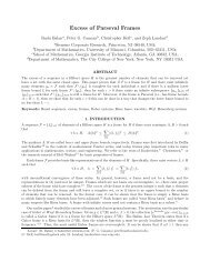
A particularly interesting example is the smallest truly redundant Parseval frame<br />
for R 2 , which is typically coined Mercedes-Benz frame. The reason for this naming<br />
becomes evident in Figure 1.
16 Peter G. Casazza, Gitta Kutyniok, and Friedrich Philipp<br />
Example 3. The Mercedes-Benz frame for R 2 is the equal-norm tight frame for R 2<br />
given by: { √ ( ) √<br />
( √3 )<br />
√<br />
( √ )}<br />
2 0 2<br />
3<br />
, 2<br />
1 3<br />
− 1 2 − 3<br />
,<br />
2<br />
3<br />
2<br />
− 1 2<br />
Note that this frame is also equi-angular.<br />
Fig. 1 Mercedes-Benz frame.<br />
For more information on the theoretical aspects of equi-angular frames we refer<br />
<strong>to</strong> [61, 92, 121, 140]. A selection of their applications is reconstrucion without phase<br />
[6, 5], erasure-resilient transmission [16, 103], and coding [137]. We also refer <strong>to</strong><br />
the chapters [157, 158] in this book.<br />
Another standard class of examples can be derived from the discrete Fourier<br />
transform (DFT) matrix.<br />
Example 4. Given M ∈ N, we let ω = exp( 2πi<br />
M<br />
). Then the discrete Fourier transform<br />
(DFT) matrix in C M×M is defined by<br />
D M = 1 √<br />
M<br />
(<br />
ω jk) M−1<br />
j,k=0 .<br />
This matrix is a unitary opera<strong>to</strong>r on C M . Later (see Corollary 11) it will be seen that<br />
the selection of any N rows from D M , yields a Parseval frame for C N by taking the<br />
associated M column vec<strong>to</strong>rs.<br />
We would like <strong>to</strong> finally mention that Section 6 contains diverse constructions<br />
of frames. There also exist particularly interesting classes of frames such as Gabor<br />
frames utilized primarily for audio processing. Among the results on various aspects<br />
of Gabor frames are uncertainty considerations [114], linear independence<br />
[120], group-related properties [90], optimality analysis [128], and applications<br />
[68, 75, 76, 88, 89]. Chapter [159] provides a survey for this class of frames. Another<br />
example is the class of group frames, for which various constructions [25, 102, 148],<br />
classifications [65], and intriguing symmetry properties [147, 149] have been studied.<br />
A comprehensive presentation can be found in Chapter [158].
<strong>Introduction</strong> <strong>to</strong> <strong>Finite</strong> <strong>Frame</strong> <strong>Theory</strong> 17<br />
4 <strong>Frame</strong>s and Opera<strong>to</strong>rs<br />
The analysis, synthesis, and frame opera<strong>to</strong>r determine the operation of a frame when<br />
analyzing and reconstructing a signal. The Grammian opera<strong>to</strong>r is perhaps not that<br />
well-known, yet it crucially illuminates the behavior of a frame (ϕ i ) M i=1 embedded<br />
as an N-dimensional subspace in the high-dimensional space R M .<br />
For the rest of this introduction we set l M 2 := l 2({1,...,M}). Note that this space<br />
in fact coincides with R M or C M , endowed with the standard inner product and the<br />
associated Euclidean norm.<br />
4.1 Analysis and Synthesis Opera<strong>to</strong>rs<br />
Two of the main opera<strong>to</strong>rs associated with a frame are the analysis and synthesis<br />
opera<strong>to</strong>rs. The analysis opera<strong>to</strong>r – as the name suggests – analyzes a signal in terms<br />
of the frame by computing its frame coefficients. We start by formalizing this notion.<br />
Definition 15. Let (ϕ i ) M i=1 be a family of vec<strong>to</strong>rs in H N . Then the associated analysis<br />
opera<strong>to</strong>r T : H N → l M 2 is defined by<br />
T x := ( 〈x,ϕ i 〉 ) M<br />
i=1 , x ∈ H N .<br />
In the following lemma we derive two basic properties of the analysis opera<strong>to</strong>r.<br />
Lemma 3. Let (ϕ i ) M i=1 be a sequence of vec<strong>to</strong>rs in H N with associated analysis<br />
opera<strong>to</strong>r T .<br />
(i) We have<br />
‖T x‖ 2 =<br />
M<br />
∑<br />
i=1<br />
|〈x,ϕ i 〉| 2 for all x ∈ H N .<br />
Hence, (ϕ i ) M i=1 is a frame for H N if and only if T is injective.<br />
(ii) The adjoint opera<strong>to</strong>r T ∗ : l M 2 → H N of T is given by<br />
T ∗ (a i ) M i=1 =<br />
M<br />
∑<br />
i=1<br />
a i ϕ i .<br />
Proof. (i). This is an immediate consequence of the definition of T and the frame<br />
property (2).<br />
(ii). For x = (a i ) M i=1 and y ∈ H N , we have<br />
〈<br />
〈T ∗ x,y〉 = 〈x,Ty〉 = (a i ) M i=1, ( 〈y,ϕ i 〉 ) 〉<br />
M<br />
i=1<br />
=<br />
M<br />
∑<br />
i=1<br />
a i 〈y,ϕ i 〉 =<br />
〈 M∑<br />
a i ϕ i ,y<br />
i=1<br />
〉<br />
.<br />
Thus, T ∗ is as claimed.<br />
⊓⊔
18 Peter G. Casazza, Gitta Kutyniok, and Friedrich Philipp<br />
The second main opera<strong>to</strong>r associated <strong>to</strong> a frame, the synthesis opera<strong>to</strong>r, is now<br />
defined as the adjoint opera<strong>to</strong>r <strong>to</strong> the analysis opera<strong>to</strong>r given in Lemma 3(ii).<br />
Definition 16. Let (ϕ i ) M i=1 be a sequence of vec<strong>to</strong>rs in H N with associated analysis<br />
opera<strong>to</strong>r T . Then the associated synthesis opera<strong>to</strong>r is defined <strong>to</strong> be the adjoint<br />
opera<strong>to</strong>r T ∗ .<br />
The next result summarizes some basic, yet useful properties of the synthesis<br />
opera<strong>to</strong>r.<br />
Lemma 4. Let (ϕ i ) M i=1 be a sequence of vec<strong>to</strong>rs in H N with associated analysis<br />
opera<strong>to</strong>r T .<br />
(i) Let (e i ) M i=1 denote the standard unit basis of lM 2 . Then for all i = 1,2,...,M, we<br />
have T ∗ e i = T ∗ Pe i = ϕ i , where P : l M 2 → lM 2 denotes the orthogonal projection<br />
on<strong>to</strong> ranT .<br />
(ii) (ϕ i ) M i=1 is a frame if and only if T ∗ is surjective.<br />
Proof. The first claim follows immediately from Lemma 3 and the fact that kerT ∗ =<br />
(ranT ) ⊥ . The second claim is a consequence of ranT ∗ = (kerT ) ⊥ and Lemma 3(i).<br />
⊓⊔<br />
Often frames are modified by the application of an invertible opera<strong>to</strong>r. The next<br />
result shows not only the impact on the associated analysis opera<strong>to</strong>r, but also the<br />
fact that the new sequence again forms a frame.<br />
Proposition 9. Let Φ = (ϕ i ) M i=1 be a sequence of vec<strong>to</strong>rs in H N with associated<br />
analysis opera<strong>to</strong>r T Φ and let F : H N → H N be a linear opera<strong>to</strong>r. Then the analysis<br />
opera<strong>to</strong>r of the sequence FΦ = (Fϕ i ) M i=1 is given by<br />
T FΦ = T Φ F ∗ .<br />
Moreover, if Φ is a frame for H N and F is invertible, then also FΦ is a frame for<br />
H N .<br />
Proof. For x ∈ H N we have<br />
T FΦ x = ( 〈x,Fϕ i 〉 ) M<br />
i=1 = ( 〈F ∗ x,ϕ i 〉 ) M<br />
i=1 = T ΦF ∗ x.<br />
This proves T FΦ = T Φ F ∗ . The moreover-part follows from Lemma 4(ii).<br />
⊓⊔<br />
Next, we analyze the structure of the matrix representation of the synthesis opera<strong>to</strong>r.<br />
This matrix is of fundamental importance, since this is what most frame<br />
constructions in fact focus on, see also Section 6.<br />
The first result provides the form of this matrix alongside with stability properties.
<strong>Introduction</strong> <strong>to</strong> <strong>Finite</strong> <strong>Frame</strong> <strong>Theory</strong> 19<br />
Lemma 5. Let (ϕ i ) M i=1 be a frame for H N with analysis opera<strong>to</strong>r T . Then a matrix<br />
representation of the synthesis opera<strong>to</strong>r T ∗ is the N × M matrix given by<br />
⎡<br />
⎣ | | ··· | ⎤<br />
ϕ 1 ϕ 2 ··· ϕ M<br />
⎦.<br />
| | ··· |<br />
Moreover, the Riesz bounds of the row vec<strong>to</strong>rs of this matrix equal the frame bounds<br />
of the column vec<strong>to</strong>rs.<br />
Proof. The form of the matrix representation is obvious. To prove the moreoverpart,<br />
let (e j ) N j=1 be the corresponding orthonormal basis of H N and for j =<br />
1,2,...,N let<br />
ψ j = [〈ϕ 1 ,e j 〉,〈ϕ 2 ,e j 〉,...,〈ϕ M ,e j 〉],<br />
be the row vec<strong>to</strong>rs of the matrix. Then for x = ∑ N j=1 a je j we obtain<br />
M<br />
∑<br />
i=1<br />
|〈x,ϕ i 〉| 2 =<br />
=<br />
M<br />
∑<br />
i=1<br />
∣<br />
N<br />
∑<br />
j,k=1<br />
N<br />
2<br />
N M a j 〈e j ,ϕ i 〉<br />
=<br />
∣<br />
∑ j a k ∑ 〈e j ,ϕ i 〉〈ϕ i ,e k 〉<br />
j,k=1a<br />
i=1<br />
∥ N ∥∥∥∥<br />
2<br />
a j a k 〈ψ k ,ψ j 〉 =<br />
∥∑<br />
a j ψ j .<br />
∑<br />
j=1<br />
j=1<br />
The claim follows from here.<br />
⊓⊔<br />
A much stronger result (Proposition 12) can be proven for the case in which the<br />
matrix representation is derived using a specifically chosen orthonormal basis. The<br />
choice of this orthonormal basis though requires the introduction of the so-called<br />
frame opera<strong>to</strong>r in the following Subsection 4.2.<br />
4.2 The <strong>Frame</strong> Opera<strong>to</strong>r<br />
The frame opera<strong>to</strong>r might be considered the most important opera<strong>to</strong>r associated with<br />
a frame. Although it is ‘merely’ the concatenation of the analysis and synthesis opera<strong>to</strong>r,<br />
it encodes crucial properties of the frame as we will see in the sequel. Moreover,<br />
it is also fundamental for the reconstruction of signals from frame coefficients<br />
(see Theorem 8).<br />
4.2.1 Fundamental Properties<br />
The precise definition of the frame opera<strong>to</strong>r associated with a frame is as follows.<br />
Definition 17. Let (ϕ i ) M i=1 be a sequence of vec<strong>to</strong>rs in H N with associated analysis<br />
opera<strong>to</strong>r T . Then the associated frame opera<strong>to</strong>r S : H N → H N is defined by
20 Peter G. Casazza, Gitta Kutyniok, and Friedrich Philipp<br />
Sx := T ∗ T x =<br />
M<br />
∑<br />
i=1<br />
〈x,ϕ i 〉ϕ i , x ∈ H N .<br />
A first observation concerning the close relation of the frame opera<strong>to</strong>r <strong>to</strong> frame<br />
properties is the following lemma.<br />
Lemma 6. Let (ϕ i ) M i=1 be a sequence of vec<strong>to</strong>rs in H N with associated frame opera<strong>to</strong>r<br />
S. Then, for all x ∈ H N ,<br />
〈Sx,x〉 =<br />
M<br />
∑<br />
i=1<br />
|〈x,ϕ i 〉| 2 .<br />
Proof. This follows directly from 〈Sx,x〉 = 〈T ∗ T x,x〉 = ‖T x‖ 2 and Lemma 3(i).<br />
⊓⊔<br />
Clearly, the frame opera<strong>to</strong>r S = T ∗ T is self-adjoint and positive. The most fundamental<br />
property of the frame opera<strong>to</strong>r – if the underlying sequence of vec<strong>to</strong>rs forms<br />
a frame – is its invertibility which is crucial for the reconstruction formula.<br />
Theorem 4. The frame opera<strong>to</strong>r S of a frame (ϕ i ) M i=1 for H N with frame bounds A<br />
and B is a positive, self-adjoint invertible opera<strong>to</strong>r satisfying<br />
Proof. By Lemma 6, we have<br />
〈Ax,x〉 = A‖x‖ 2 ≤<br />
M<br />
∑<br />
i=1<br />
A · Id ≤ S ≤ B · Id.<br />
|〈x,ϕ i 〉| 2 = 〈Sx,x〉 ≤ B‖x‖ 2 = 〈Bx,x〉 for all x ∈ H N .<br />
This implies the claimed inequality.<br />
⊓⊔<br />
The following proposition follows directly from Proposition 9.<br />
Proposition 10. Let (ϕ i ) M i=1 be a frame for H N with frame opera<strong>to</strong>r S, and let F be<br />
an invertible opera<strong>to</strong>r on H N . Then (Fϕ i ) M i=1 is a frame with frame opera<strong>to</strong>r FSF∗ .<br />
4.2.2 The Special Case of Tight <strong>Frame</strong>s<br />
Tight frames can be characterized as those frames whose frame opera<strong>to</strong>r equals a<br />
positive multiple of the identity. The next result provides a variety of similarly frame<br />
opera<strong>to</strong>r inspired classifications.<br />
Proposition 11. Let (ϕ i ) M i=1 be a frame for H N with analysis opera<strong>to</strong>r T and frame<br />
opera<strong>to</strong>r S. Then the following conditions are equivalent.<br />
(i) (ϕ i ) M i=1 is an A-tight frame for H N .<br />
(ii) S = A · Id.
<strong>Introduction</strong> <strong>to</strong> <strong>Finite</strong> <strong>Frame</strong> <strong>Theory</strong> 21<br />
(iii) For every x ∈ H N ,<br />
(iv) For every x ∈ H N ,<br />
(v) T / √ A is an isometry.<br />
x = A −1 ·<br />
A‖x‖ 2 =<br />
M<br />
∑<br />
i=1<br />
M<br />
∑<br />
i=1<br />
〈x,ϕ i 〉ϕ i .<br />
|〈x,ϕ i 〉| 2 .<br />
Proof. (i) ⇔ (ii) ⇔ (iii) ⇔ (iv). These are immediate from the definition of the<br />
frame opera<strong>to</strong>r and from Theorem 4.<br />
(ii) ⇔ (v). This follows from the fact that T / √ A is an isometry if and only if<br />
T ∗ T = A · Id. ⊓⊔<br />
A similar result for the special case of a Parseval frame can be easily deduced<br />
from Proposition 11 by setting A = 1.<br />
4.2.3 Eigenvalues of the <strong>Frame</strong> Opera<strong>to</strong>r<br />
Tight frames have the property that the eigenvalues of the associated frame opera<strong>to</strong>r<br />
all coincide. We next consider the general situation, i.e., frame opera<strong>to</strong>rs with<br />
arbitrary eigenvalues.<br />
The first and maybe even most important result shows that the largest and smallest<br />
eigenvalues of the frame opera<strong>to</strong>r are the optimal frame bounds of the frame.<br />
Optimality refers <strong>to</strong> the smallest upper frame bound and the largest lower frame<br />
bound.<br />
Theorem 5. Let (ϕ i ) M i=1 be a frame for H N with frame opera<strong>to</strong>r S having eigenvalues<br />
λ 1 ≥ ... ≥ λ N . Then λ 1 coincides with the optimal upper frame bound and λ N<br />
is the optimal lower frame bound.<br />
Proof. Let (e i ) N i=1<br />
denote the normalized eigenvec<strong>to</strong>rs of the frame opera<strong>to</strong>r S with<br />
respective eigenvalues (λ j ) N j=1 written in decreasing order. Let x ∈ H N be arbitrarily<br />
fixed. Since x = ∑ M j=1 〈x,e j〉e j , we obtain<br />
By Lemma 6, this implies<br />
M<br />
∑<br />
i=1<br />
Sx =<br />
|〈x,ϕ i 〉| 2 = 〈Sx,x〉 =<br />
=<br />
N<br />
∑<br />
j=1<br />
〈 N∑<br />
j=1<br />
λ j 〈x,e j 〉e j .<br />
λ j 〈x,e j 〉e j ,<br />
N<br />
∑<br />
j=1<br />
〈x,e j 〉e j<br />
〉<br />
N<br />
∑ j |〈x,e j 〉|<br />
j=1λ 2 N<br />
≤ λ 1 ∑ |〈x,e j 〉| 2 = λ 1 ‖x‖ 2 .<br />
j=1
22 Peter G. Casazza, Gitta Kutyniok, and Friedrich Philipp<br />
Thus B op ≤ λ 1 , where B op denotes the optimal upper frame bound of the frame<br />
(ϕ i ) M i=1 . The claim B op = λ 1 then follows from<br />
M<br />
∑<br />
i=1<br />
|〈e 1 ,ϕ i 〉| 2 = 〈Se 1 ,e 1 〉 = 〈λ 1 e 1 ,e 1 〉 = λ 1 .<br />
The claim concerning the lower frame bound can be proven similarly.<br />
From this result, we can now draw the following immediate conclusion on Riesz<br />
bounds.<br />
Corollary 6. Let (ϕ i ) N i=1 be a frame for H N . Then the following statements hold.<br />
(i) The optimal upper Riesz bound and the optimal upper frame bound of (ϕ i ) N i=1<br />
coincide.<br />
(ii) The optimal lower Riesz bound and the optimal lower frame bound of (ϕ i ) N i=1<br />
coincide.<br />
Proof. Let T denote the analysis opera<strong>to</strong>r of (ϕ i ) N i=1<br />
and S the associated frame<br />
opera<strong>to</strong>r having eigenvalues (λ i ) N i=1<br />
written in decreasing order. We have<br />
and<br />
λ 1 = ‖S‖ = ‖T ∗ T ‖ = ‖T ‖ 2 = ‖T ∗ ‖ 2<br />
λ N = ‖S −1 ‖ −1 = ‖(T ∗ T ) −1 ‖ −1 = ‖(T ∗ ) −1 ‖ −2 .<br />
Now, both claims follow from Theorem 5, Lemma 4, and Proposition 5.<br />
The next theorem reveals a relation between the frame vec<strong>to</strong>rs and the eigenvalues<br />
and eigenvec<strong>to</strong>rs of the associated frame opera<strong>to</strong>r.<br />
Theorem 6. Let (ϕ i ) M i=1 be a frame for H N with frame opera<strong>to</strong>r S having normalized<br />
eigenvec<strong>to</strong>rs (e j ) N j=1 and respective eigenvalues (λ j) N j=1<br />
. Then for all j =<br />
1,2,...,N we have<br />
In particular,<br />
λ j =<br />
TrS =<br />
M<br />
∑<br />
i=1<br />
N<br />
∑<br />
j=1<br />
|〈e j ,ϕ i 〉| 2 .<br />
λ j =<br />
M<br />
∑<br />
i=1<br />
‖ϕ i ‖ 2 .<br />
Proof. This follows from λ j = 〈Se j ,e j 〉 for all j = 1,...,N and Lemma 6.<br />
⊓⊔<br />
⊓⊔<br />
⊓⊔<br />
4.2.4 Structure of the Synthesis Matrix<br />
As already promised in Subsection 4.1, we now apply the previously derived results<br />
<strong>to</strong> obtain a complete characterization of the synthesis matrix of a frame in terms of<br />
the frame opera<strong>to</strong>r.
<strong>Introduction</strong> <strong>to</strong> <strong>Finite</strong> <strong>Frame</strong> <strong>Theory</strong> 23<br />
Proposition 12. Let T : H N → l M 2 be a linear opera<strong>to</strong>r, let (e j) N j=1<br />
be an orthonormal<br />
basis of H N and let (λ j ) N j=1<br />
be a sequence of positive numbers. By A denote<br />
the N ×M matrix representation of T ∗ with respect <strong>to</strong> (e j ) N j=1<br />
(and the standard unit<br />
basis (ê i ) M i=1 of lM 2 ). Then the following conditions are equivalent.<br />
(i) (T ∗ ê i ) M i=1 forms a frame for H N whose frame opera<strong>to</strong>r has eigenvec<strong>to</strong>rs (e j ) N j=1<br />
and associated eigenvalues (λ j ) N j=1 .<br />
(ii) The rows of A are orthogonal, and the j-th row square sums <strong>to</strong> λ j .<br />
(iii) The columns of A form a frame for l N 2 , and AA∗ = diag(λ 1 ,...,λ N ).<br />
Proof. Let ( f j ) N j=1 be the standard unit basis of lN 2 and denote by U : lN 2 → H N the<br />
unitary opera<strong>to</strong>r which maps f j <strong>to</strong> e j . Then T ∗ = UA.<br />
(i)⇒(ii). For j,k ∈ {1,...,N} we have<br />
〈A ∗ f j ,A ∗ f k 〉 = 〈TU f j ,TU f k 〉 = 〈T ∗ Te j ,e k 〉 = λ j δ jk ,<br />
which is equivalent <strong>to</strong> (ii).<br />
(ii)⇒(iii). Since the rows of A are orthogonal, we have rankA = N which implies<br />
that the columns of A form a frame for l N 2 . The rest follows from 〈AA∗ f j , f k 〉 =<br />
〈A ∗ f j ,A ∗ f k 〉 = λ j δ jk for j,k = 1,...,N.<br />
(iii)⇒(i). Since (Aê i ) M i=1 is a spanning set for lN 2<br />
and T ∗ = UA, it follows that<br />
(T ∗ ê i ) M i=1 forms a frame for H N . Its analysis opera<strong>to</strong>r is given by T since for all<br />
x ∈ H N ,<br />
(〈x,T ∗ ê i 〉) M i=1 = (〈T x,ê i 〉) M i=1 = T x.<br />
Moreover,<br />
T ∗ Te j = UAA ∗ U ∗ e j = U diag(λ 1 ,...,λ N ) f j = λ j U f j = λ j e j ,<br />
which completes the proof.<br />
⊓⊔<br />
4.3 Grammian Opera<strong>to</strong>r<br />
Let (ϕ i ) M i=1 be a frame for H N with analysis opera<strong>to</strong>r T . The previous subsection<br />
was concerned with properties of the frame opera<strong>to</strong>r defined by S = T ∗ T : H N →<br />
H N . Of particular interest is also the opera<strong>to</strong>r generated by first applying the synthesis<br />
and then the analysis opera<strong>to</strong>r. Let us first state the precise definition before<br />
discussing its importance.<br />
Definition 18. Let (ϕ i ) M i=1 be a frame for H N with analysis opera<strong>to</strong>r T . Then the<br />
opera<strong>to</strong>r G : l M 2 → lM 2 defined by<br />
G(a i ) M i=1 = T T ∗ (a i ) M i=1 =<br />
( M∑<br />
) M<br />
a i 〈ϕ i ,ϕ k 〉<br />
i=1<br />
k=1<br />
=<br />
M<br />
∑<br />
i=1<br />
a i (〈ϕ i ,ϕ k 〉) M k=1
24 Peter G. Casazza, Gitta Kutyniok, and Friedrich Philipp<br />
is called the Grammian (opera<strong>to</strong>r) of the frame (ϕ i ) M i=1 .<br />
Note that the (canonical) matrix representation of the Grammian of a frame<br />
(ϕ i ) M i=1 for H N (which will also be called the Grammian matrix) is given by<br />
⎡<br />
‖ϕ 1 ‖ 2 ⎤<br />
〈ϕ 2 ,ϕ 1 〉 ··· 〈ϕ M ,ϕ 1 〉<br />
〈ϕ 1 ,ϕ 2 〉 ‖ϕ 2 ‖ 2 ··· 〈ϕ M ,ϕ 2 〉<br />
⎢<br />
⎣<br />
.<br />
. . ..<br />
⎥<br />
. ⎦ .<br />
〈ϕ 1 ,ϕ M 〉 〈ϕ 2 ,ϕ M 〉 ··· ‖ϕ M ‖ 2<br />
One property of the Grammian is immediate. In fact, if the frame is unit-norm then<br />
the entries of the Grammian matrix are exactly the cosines of the angles between the<br />
frame vec<strong>to</strong>rs. Hence, for instance, if a frame is equi-angular then all off diagonal<br />
entries of the Grammian matrix have the same modulus.<br />
The fundamental properties of the Grammian opera<strong>to</strong>r are collected in the following<br />
result.<br />
Theorem 7. Let (ϕ i ) M i=1 be a frame for H N with analysis opera<strong>to</strong>r T , frame opera<strong>to</strong>r<br />
S, and Grammian opera<strong>to</strong>r G. Then the following statements hold.<br />
(i) An opera<strong>to</strong>r U on H N is unitary if and only if the Grammian of (Uϕ i ) M i=1 coincides<br />
with G.<br />
(ii) The non-zero eigenvalues of G and S coincide.<br />
(iii) (ϕ i ) M i=1 is a Parseval frame if and only if G is an orthogonal projection of rank N<br />
(namely on<strong>to</strong> the range of T ).<br />
(iv) G is invertible if and only if M = N.<br />
Proof. (i). This follows immediately from the fact that the entries of the Grammian<br />
matrix for (Uϕ i ) M i=1 are of the form 〈Uϕ i,Uϕ j 〉.<br />
(ii). Since T T ∗ and T ∗ T have the same non-zero eigenvalues (see Proposition 7),<br />
the same is true for G and S.<br />
(iii). It is immediate <strong>to</strong> prove that G is self-adjoint and has rank N. Since T is<br />
injective, T ∗ is surjective, and<br />
G 2 = (T T ∗ )(T T ∗ ) = T (T ∗ T )T ∗ ,<br />
it follows that G is an orthogonal projection if and only if T ∗ T = Id, which is equivalent<br />
<strong>to</strong> the frame being Parseval.<br />
(iv). This is immediate by (ii). ⊓⊔<br />
5 Reconstruction from <strong>Frame</strong> Coefficients<br />
The analysis of a signal is typically performed by merely considering its frame<br />
coefficients. However, if the task is transmission of a signal, the ability <strong>to</strong> reconstruct<br />
the signal from its frame coefficients and also <strong>to</strong> do so efficiently becomes crucial.
<strong>Introduction</strong> <strong>to</strong> <strong>Finite</strong> <strong>Frame</strong> <strong>Theory</strong> 25<br />
Reconstruction from coefficients with respect <strong>to</strong> an orthonormal basis was already<br />
discussed in Corollary 1. However, reconstruction from coefficients with respect <strong>to</strong><br />
a redundant system is much more delicate and requires the utilization of another<br />
frame, called dual frame. If computing such a dual frame is computationally <strong>to</strong>o<br />
complex, a circumvention of this problem is the so-called frame algorithm.<br />
5.1 Exact Reconstruction<br />
We start with stating an exact reconstruction formula.<br />
Theorem 8. Let (ϕ i ) M i=1 be a frame for H N with frame opera<strong>to</strong>r S. Then, for every<br />
x ∈ H N , we have<br />
x =<br />
M<br />
∑<br />
i=1<br />
〈x,ϕ i 〉S −1 ϕ i =<br />
M<br />
∑<br />
i=1<br />
〈x,S −1 ϕ i 〉ϕ i .<br />
Proof. This follows directly from the definition of the frame opera<strong>to</strong>r in Definition<br />
17 by writing x = S −1 Sx and x = SS −1 x. ⊓⊔<br />
Notice that the first formula can be interpreted as a reconstruction strategy,<br />
whereas the second formula has the flavor of a decomposition. We further observe<br />
that the sequence (S −1 ϕ i ) M i=1 plays a crucial role in the formulas in Theorem 8. The<br />
next result shows that this sequence indeed also constitutes a frame.<br />
Proposition 13. Let (ϕ i ) M i=1 be a frame for H N with frame bounds A and B and<br />
with frame opera<strong>to</strong>r S. Then the sequence (S −1 ϕ i ) M i=1 is a frame for H N with frame<br />
bounds B −1 and A −1 and with frame opera<strong>to</strong>r S −1 .<br />
Proof. By Proposition 10, the sequence (S −1 ϕ i ) M i=1 forms a frame for H N with<br />
associated frame opera<strong>to</strong>r S −1 S(S −1 ) ∗ = S −1 . This in turn yields the frame bounds<br />
B −1 and A −1 . ⊓⊔<br />
This new frame is called the canonical dual frame. In the sequel, we will discuss<br />
that also other dual frames may be utilized for reconstruction.<br />
Definition 19. Let (ϕ i ) M i=1 be a frame for H N with frame opera<strong>to</strong>r denoted by S.<br />
Then (S −1 ϕ i ) M i=1 is called the canonical dual frame for (ϕ i) M i=1 .<br />
The canonical dual frame of a Parseval frame is now easily determined by Proposition<br />
13.<br />
Corollary 7. Let (ϕ i ) M i=1 be a Parseval frame for H N . Then its canonical dual<br />
frame is the frame (ϕ i ) M i=1 itself, and the reconstruction formula in Theorem 8 reads<br />
x =<br />
M<br />
∑<br />
i=1<br />
〈x,ϕ i 〉ϕ i , x ∈ H N .
26 Peter G. Casazza, Gitta Kutyniok, and Friedrich Philipp<br />
As an application of the above reconstruction formula for Parseval frames, we<br />
prove the following proposition which again shows the close relation between Parseval<br />
frames and orthonormal bases already indicated in Lemma 2.<br />
Proposition 14 (Trace Formula for Parseval <strong>Frame</strong>s). Let (ϕ i ) M i=1 be a Parseval<br />
frame for H N , and let F be a linear opera<strong>to</strong>r on H N . Then<br />
Tr(F) =<br />
M<br />
∑<br />
i=1<br />
〈Fϕ i ,ϕ i 〉.<br />
Proof. Let (e j ) N j=1 be an orthonormal basis for H N . Then, by definition,<br />
This implies<br />
Tr(F) =<br />
N<br />
∑<br />
j=1<br />
〈Fe j ,e j 〉.<br />
Tr(F) =<br />
=<br />
N M∑<br />
〉<br />
∑ 〈Fe j ,ϕ i 〉ϕ i ,e j =<br />
j=1〈<br />
i=1<br />
M<br />
∑<br />
i=1〈<br />
N∑<br />
j=1<br />
〈ϕ i ,e j 〉e j ,F ∗ ϕ i<br />
〉<br />
=<br />
N<br />
M<br />
∑ ∑<br />
j=1 i=1<br />
M<br />
∑<br />
i=1<br />
〈e j ,F ∗ ϕ i 〉〈ϕ i ,e j 〉<br />
〈ϕ i ,F ∗ ϕ i 〉 =<br />
M<br />
∑<br />
i=1<br />
〈Fϕ i ,ϕ i 〉.<br />
⊓⊔<br />
As already announced, many other dual frames for reconstruction exist. We next<br />
provide a precise definition.<br />
Definition 20. Let (ϕ i ) M i=1 be a frame for H N . Then a frame (ψ i ) M i=1 is called a dual<br />
frame for (ϕ i ) M i=1 , if x =<br />
M<br />
∑<br />
i=1<br />
〈x,ϕ i 〉ψ i for all x ∈ H N .<br />
Dual frames, which do not coincide with the canonical dual frame, are often coined<br />
alternate dual frames.<br />
Similar <strong>to</strong> the different forms of the reconstruction formula in Theorem 8, also<br />
dual frames can achieve reconstruction in different ways.<br />
Proposition 15. Let (ϕ i ) M i=1 and (ψ i) M i=1 be frames for H N and let T and ˜T be the<br />
analysis opera<strong>to</strong>rs of (ϕ i ) M i=1 and (ψ i) M i=1 , respectively. Then the following conditions<br />
are equivalent.<br />
(i) We have x = ∑ M i=1 〈x,ψ i〉ϕ i for all x ∈ H N .<br />
(ii) We have x = ∑ M i=1 〈x,ϕ i〉ψ i for all x ∈ H N .<br />
(iii) We have 〈x,y〉 = ∑ M i=1 〈x,ϕ i〉〈ψ i ,y〉 for all x,y ∈ H N .<br />
(iv) T ∗ ˜T = Id and ˜T ∗ T = Id.
<strong>Introduction</strong> <strong>to</strong> <strong>Finite</strong> <strong>Frame</strong> <strong>Theory</strong> 27<br />
Proof. Clearly (i) is equivalent <strong>to</strong> T ∗ ˜T = Id which holds if and only if ˜T ∗ T = Id.<br />
The equivalence of (iii) can be derived in a similar way. ⊓⊔<br />
One might ask what distinguishes the canonical dual frame from the alternate<br />
dual frames besides its explicit formula in terms of the initial frame. Another seemingly<br />
different question is which properties of the coefficient sequence in the decomposition<br />
of some signal x in terms of the frame (see Theorem 8),<br />
x =<br />
M<br />
∑<br />
i=1<br />
〈x,S −1 ϕ i 〉ϕ i ,<br />
uniquely distinguishes it from other coefficient sequences – redundancy allows infinitely<br />
many coefficient sequences. Interestingly, the next result answers both questions<br />
simultaneously by stating that this coefficient sequence has minimal l 2 -norm<br />
among all sequences – in particular those, with respect <strong>to</strong> alternate dual frames –<br />
representing x.<br />
Proposition 16. Let (ϕ i ) M i=1 be a frame for H N with frame opera<strong>to</strong>r S, and let x ∈<br />
H N . If (a i ) M i=1 are scalars such that x = ∑M i=1 a iϕ i , then<br />
M<br />
∑<br />
i=1<br />
|a i | 2 =<br />
M<br />
∑<br />
i=1<br />
|〈x,S −1 ϕ i 〉| 2 +<br />
M<br />
∑<br />
i=1<br />
|a i − 〈x,S −1 ϕ i 〉| 2 .<br />
Proof. Letting T denote the analysis opera<strong>to</strong>r of (ϕ i ) M i=1 , we obtain<br />
Since x = ∑ M i=1 a iϕ i , it follows that<br />
Considering the decomposition<br />
(〈x,S −1 ϕ i 〉) M i=1 = (〈S −1 x,ϕ i 〉) M i=1 ∈ ranT.<br />
(a i − 〈x,S −1 ϕ i 〉) M i=1 ∈ kerT ∗ = (ranT ) ⊥ .<br />
(a i ) M i=1 = (〈x,S −1 ϕ i 〉) M i=1 + (a i − 〈x,S −1 ϕ i 〉) M i=1,<br />
the claim is immediate.<br />
⊓⊔<br />
Corollary 8. Let (ϕ i ) M i=1 be a frame for H N , and let (ψ i ) M i=1 be an associated alternate<br />
dual frame. Then, for all x ∈ H N ,<br />
‖(〈x,S −1 ϕ i 〉) M i=1‖ 2 ≤ ‖(〈x,ψ i 〉) M i=1‖ 2 .<br />
We wish <strong>to</strong> mention that also sequences which are minimal in the l 1 norm play a<br />
crucial role <strong>to</strong> date due <strong>to</strong> the fact that the l 1 norm promotes sparsity. The interested<br />
reader is referred <strong>to</strong> Chapter [162] for further details.
28 Peter G. Casazza, Gitta Kutyniok, and Friedrich Philipp<br />
5.2 Properties of Dual <strong>Frame</strong>s<br />
While focussing on properties of the canonical dual frame in the last subsection, we<br />
next discuss properties shared by all dual frames. The first question arising is: How<br />
do you characterize all dual frames? A comprehensive answer is provided by the<br />
following result.<br />
Proposition 17. Let (ϕ i ) M i=1 be a frame for H N with analysis opera<strong>to</strong>r T and frame<br />
opera<strong>to</strong>r S. Then the following conditions are equivalent.<br />
(i) (ψ i ) M i=1 is a dual frame for (ϕ i) M i=1 .<br />
(ii) The analysis opera<strong>to</strong>r T 1 of the sequence (ψ i − S −1 ϕ i ) M i=1 satisfies<br />
ranT ⊥ ran T 1 .<br />
Proof. We set ˜ϕ i := ψ i − S −1 ϕ i for i = 1,...,M and note that<br />
M<br />
∑<br />
i=1<br />
〈x,ψ i 〉ϕ i =<br />
M<br />
∑<br />
i=1<br />
〈x, ˜ϕ i + S −1 ϕ i 〉ϕ i = x +<br />
M<br />
∑<br />
i=1<br />
〈x, ˜ϕ i 〉ϕ i = x + T ∗ T 1 x<br />
holds for all x ∈ H N . Hence, (ψ i ) M i=1 is a dual frame for (ϕ i) M i=1<br />
T ∗ T 1 = 0. But this is equivalent <strong>to</strong> (ii). ⊓⊔<br />
if and only if<br />
From this result, we have the following corollary which provides a general formula<br />
for all dual frames.<br />
Corollary 9. Let (ϕ i ) M i=1 be a frame for H N with analysis opera<strong>to</strong>r T and frame<br />
opera<strong>to</strong>r S with associated normalized eigenvec<strong>to</strong>rs (e j ) N j=1<br />
and respective eigenvalues<br />
(λ j ) N j=1 . Then every dual frame {ψ i} M i=1 for (ϕ i) M i=1 is of the form<br />
ψ i =<br />
N<br />
∑<br />
j=1<br />
( 1<br />
λ j<br />
〈ϕ i ,e j 〉 + h i j<br />
)<br />
e j ,<br />
i = 1,...,M,<br />
where each (h i j ) M i=1 , j = 1,...,N, is an element of (ranT )⊥ .<br />
Proof. If ψ i , i = 1,...,M, is of the given form with sequences (h i j ) M i=1 ∈ lM 2 ,<br />
j = 1,...,N, then ψ i = S −1 ϕ i + ˜ϕ i , where ˜ϕ i := ∑ N j=1 h i je j , i = 1,...,M. The analysis<br />
opera<strong>to</strong>r ˜T of ( ˜ϕ i ) M i=1 satisfies ˜T e j = (h i j ) M i=1 . The claim follows from this observation.<br />
⊓⊔<br />
As a second corollary, we derive a characterization of all frames which have a<br />
uniquely determined dual frame. It is evident, that this unique dual frame coincides<br />
with the canonical dual frame.<br />
Corollary 10. A frame (ϕ i ) M i=1 for H N has a unique dual frame if and only if M =<br />
N.
<strong>Introduction</strong> <strong>to</strong> <strong>Finite</strong> <strong>Frame</strong> <strong>Theory</strong> 29<br />
5.3 <strong>Frame</strong> Algorithms<br />
Let (ϕ i ) M i=1 be a frame for H N with frame opera<strong>to</strong>r S, and assume we are given the<br />
image of a signal x ∈ H N under the analysis opera<strong>to</strong>r, i.e., the sequence (〈x,ϕ i 〉) M i=1<br />
in l M 2 . Theorem 8 already provided us with the reconstruction formula<br />
x =<br />
M<br />
∑<br />
i=1<br />
〈x,ϕ i 〉S −1 ϕ i<br />
by using the canonical dual frame. Since inversion is typically not only computationally<br />
expensive, but also numerically instable, this formula might not be utilizable<br />
in practice.<br />
To resolve this problem, we will next discuss three iterative methods <strong>to</strong> derive<br />
a converging sequence of approximations of x from knowledge of (〈x,ϕ i 〉) M i=1 . The<br />
first on our list is the so-called frame algorithm.<br />
Proposition 18 (<strong>Frame</strong> Algorithm). Let (ϕ i ) M i=1 be a frame for H N with frame<br />
bounds A,B and frame opera<strong>to</strong>r S. Given a signal x ∈ H N , define a sequence<br />
(y j ) ∞ j=0 in H N by<br />
y 0 = 0, y j = y j−1 + 2<br />
A + B S(x − y j−1) for all j ≥ 1.<br />
Then (y j ) ∞ j=0 converges <strong>to</strong> x in H N and the rate of convergence is<br />
‖x − y j ‖ ≤<br />
Proof. First, for all x ∈ H N , we have<br />
〈(<br />
Id − 2 ) 〉<br />
A + B S x,x = ‖x‖ 2 − 2<br />
A + B<br />
Similarly, we obtain<br />
which yields<br />
By the definition of y j , for any j ≥ 0,<br />
( ) B − A j<br />
‖x‖, j ≥ 0.<br />
B + A<br />
M<br />
∑<br />
i=1<br />
|〈x,ϕ i 〉| 2 ≤ ‖x‖ 2 − 2A<br />
A + B ‖x‖2 = B − A<br />
A + B ‖x‖2 .<br />
− B − A 〈(<br />
B + A ‖x‖2 ≤ Id − 2 ) 〉<br />
A + B S x,x ,<br />
∥<br />
∥Id − 2<br />
A + B S ∥ ∥∥ ≤<br />
B − A<br />
A + B . (3)<br />
x − y j = x − y j−1 − 2<br />
(<br />
A + B S(x − y j−1) = Id − 2 )<br />
A + B S (x − y j−1 ).<br />
Iterating this calculation, we derive
30 Peter G. Casazza, Gitta Kutyniok, and Friedrich Philipp<br />
Thus, by (3),<br />
The result is proved.<br />
(<br />
x − y j = Id − 2 ) j(x<br />
A + B S − y0 ), for all j ≥ 0.<br />
(<br />
‖x − y j ‖ = ∥ Id − 2 ) j(x A + B S − y0 ) ∥<br />
∥<br />
≤ ∥Id − 2 ∥ ∥∥<br />
A + B S j<br />
‖x − y0 ‖<br />
( B − A<br />
) j‖x‖.<br />
≤<br />
A + B<br />
⊓⊔<br />
We wish <strong>to</strong> mention that, although the iteration formula in the frame algorithm<br />
contains x, the algorithm does not depend on the knowledge of x but only on the<br />
frame coefficients (〈x,ϕ i 〉) M i=1 , since y j = y j−1 +<br />
A+B 2 (∑ i〈x,ϕ i 〉ϕ i − Sy j−1 ).<br />
One drawback of the frame algorithm is the fact that not only does the convergence<br />
rate depend on the ratio of the frame bounds, i.e., the condition number of the<br />
frame, but it depends on it in a highly sensitive way. This causes the problem that a<br />
large ratio of the frame bounds leads <strong>to</strong> very slow convergence.<br />
To tackle this problem, in [97], the Chebyshev method and the conjugate gradient<br />
methods were introduced, which are significantly better adapted <strong>to</strong> frame theory<br />
leading <strong>to</strong> faster convergence than the frame algorithm. These two algorithms will<br />
next be discussed. We start with the Chebyshev algorithm.<br />
Proposition 19 (Chebychev Algorithm, [97]). Let (ϕ i ) M i=1 be a frame for H N with<br />
frame bounds A,B and frame opera<strong>to</strong>r S, and set<br />
ρ := B − A<br />
B + A and σ := √<br />
B −<br />
√<br />
A<br />
√<br />
B +<br />
√<br />
A<br />
.<br />
Given a signal x ∈ H N , define a sequence (y j ) ∞ j=0 in H N and corresponding<br />
scalars (λ j ) ∞ j=1 by y 0 = 0, y 1 = 2<br />
B + A Sx, and λ 1 = 2,<br />
and for j ≥ 2, set<br />
λ j =<br />
1<br />
1 − ρ2<br />
4 λ j−1<br />
and y j = λ j<br />
(<br />
y j−1 − y j−2 + 2<br />
B + A S (<br />
x − y j−1<br />
))<br />
+ y j−2 .<br />
Then (y j ) ∞ j=0 converges <strong>to</strong> x in H N and the rate of convergence is<br />
‖x − y j ‖ ≤<br />
2σ j<br />
1 + σ 2 j ‖x‖.
<strong>Introduction</strong> <strong>to</strong> <strong>Finite</strong> <strong>Frame</strong> <strong>Theory</strong> 31<br />
The advantage of the conjugate gradient method, which we will present next, is<br />
the fact that it does not require knowledge of the frame bounds. However, as before,<br />
the rate of convergence certainly does depend on them.<br />
Proposition 20 (Conjugate Gradient Method, [97]). Let (ϕ i ) M i=1 be a frame for<br />
H N with frame opera<strong>to</strong>r S. Given a signal x ∈ H N , define three sequences (y j ) ∞ j=0 ,<br />
(r j ) ∞ j=0 , and (p j) ∞ j=−1 in H N and corresponding scalars (λ j ) ∞ j=−1 by<br />
and for j ≥ 0, set<br />
and<br />
y 0 = 0, r 0 = p 0 = Sx, and p −1 = 0,<br />
λ j = 〈r j, p j 〉<br />
〈p j ,Sp j 〉 , y j+1 = y j + λ j p j , r j+1 = r j − λ j Sp j ,<br />
p j+1 = Sp j − 〈Sp j,Sp j 〉<br />
〈p j ,Sp j 〉 p j − 〈Sp j,Sp j−1 〉<br />
〈p j−1 ,Sp j−1 〉 p j−1.<br />
Then (y j ) ∞ j=0 converges <strong>to</strong> x in H N and the rate of convergence is<br />
|||x − y j ||| ≤<br />
2σ j<br />
1 + σ 2 j |||x||| with σ = √<br />
B −<br />
√<br />
A<br />
√<br />
B +<br />
√<br />
A<br />
,<br />
and ||| · ||| is the norm on H N given by |||x||| = 〈x,Sx〉 1/2 = ‖S 1/2 x‖, x ∈ H N .<br />
6 Construction of <strong>Frame</strong>s<br />
As diverse as the various desiderata are which applications require a frame <strong>to</strong> satisfy,<br />
as diverse are also the methods <strong>to</strong> construct frames [37, 59]. In this section,<br />
we will present a prominent selection. For further details and results, such as, for<br />
example, the construction of frames through spectral tetris [31, 47, 44] and through<br />
eigensteps [30], we refer <strong>to</strong> Chapter [155].<br />
6.1 Tight and Parseval <strong>Frame</strong>s<br />
Tight frames are particularly desirable due <strong>to</strong> the fact that the reconstruction of<br />
a signal from tight frame coefficients is numerically optimally stable as already<br />
discussed in Section 5. Most of the constructions we will present utilize a given<br />
frame, which is then modified <strong>to</strong> become a tight frame.<br />
We start with the most basic result for generating a Parseval frame which is the<br />
application of S −1/2 , S being the frame opera<strong>to</strong>r.
32 Peter G. Casazza, Gitta Kutyniok, and Friedrich Philipp<br />
Lemma 7. If (ϕ i ) M i=1 is a frame for H N with frame opera<strong>to</strong>r S, then (S −1/2 ϕ i ) M i=1 is<br />
a Parseval frame.<br />
Proof. By Proposition 10, the frame opera<strong>to</strong>r for (S −1/2 ϕ i ) M i=1 is S−1/2 SS −1/2 = Id.<br />
⊓⊔<br />
Although this result is impressive in its simplicity, from a practical point of view<br />
it has various problems, the most significant being that this procedure requires inversion<br />
of the frame opera<strong>to</strong>r.<br />
However, Lemma 7 can certainly be applied if all eigenvalues and respective<br />
eigenvec<strong>to</strong>rs of the frame opera<strong>to</strong>r are given. If only information on the eigenspace<br />
corresponding <strong>to</strong> the largest eigenvalue is missing, then there exists a simple practical<br />
method <strong>to</strong> generate a tight frame by adding a provably minimal number of<br />
vec<strong>to</strong>rs.<br />
Proposition 21. Let (ϕ i ) M i=1 be any family of vec<strong>to</strong>rs in H N with frame opera<strong>to</strong>r<br />
S having eigenvec<strong>to</strong>rs (e j ) N j=1 and respective eigenvalues λ 1 ≥ λ 2 ≥ ... ≥ λ N . Let<br />
1 ≤ k ≤ N be such that λ 1 = λ 2 = ... = λ k > λ k+1 . Then<br />
(<br />
) N<br />
(ϕ i ) M i=1 ∪ (λ 1 − λ j ) 1/2 e j<br />
j=k+1<br />
forms a λ 1 -tight frame for H N .<br />
Moreover, N − k is the least number of vec<strong>to</strong>rs which can be added <strong>to</strong> (ϕ i ) M i=1 <strong>to</strong><br />
obtain a tight frame.<br />
Proof. A straightforward calculation shows that the sequence in (4) is indeed a λ 1 -<br />
tight frame for H N .<br />
For the moreover-part, assume that there exist vec<strong>to</strong>rs (ψ j ) j∈J with frame opera<strong>to</strong>r<br />
S 1 satisfying that (ϕ i ) M i=1 ∪ (ψ j) j∈J is an A-tight frame. This implies A ≥ λ 1 .<br />
Now define S 2 <strong>to</strong> be the opera<strong>to</strong>r on H N given by<br />
{<br />
0 : 1 ≤ j ≤ k,<br />
S 2 e j =<br />
(λ 1 − λ j )e j : k + 1 ≤ j ≤ N.<br />
It follows that A · Id = S + S 1 and<br />
S 1 = A · Id − S ≥ λ 1 Id − S = S 2 .<br />
Since S 2 has N − k non-zero eigenvalues, also S 1 has at least N − k non-zero eigenvalues.<br />
Hence |J| ≥ N − k, showing that indeed N − k added vec<strong>to</strong>rs is minimal.<br />
⊓⊔<br />
Before we delve in<strong>to</strong> further explicit constructions, we need <strong>to</strong> first state some<br />
fundamental results on tight, and, in particular, Parseval frames.<br />
The most basic invariance property a frame could have is invariance under orthogonal<br />
projections. The next result shows that this operation indeed maintains<br />
and may even improve the frame bounds. In particular, the orthogonal projection of<br />
a Parseval frame remains a Parseval frame.<br />
(4)
<strong>Introduction</strong> <strong>to</strong> <strong>Finite</strong> <strong>Frame</strong> <strong>Theory</strong> 33<br />
Proposition 22. Let (ϕ i ) M i=1 be a frame for H N with frame bounds A,B, and let P<br />
be an orthogonal projection of H N on<strong>to</strong> a subspace W . Then (Pϕ i ) M i=1 is a frame<br />
for W with frame bounds A,B.<br />
In particular, if (ϕ i ) M i=1 is a Parseval frame for H N and P is an orthogonal<br />
projection on H N on<strong>to</strong> W , then (Pϕ i ) M i=1 is a Parseval frame for W .<br />
Proof. For any x ∈ W ,<br />
A‖x‖ 2 = A‖Px‖ 2 ≤<br />
M<br />
∑<br />
i=1<br />
|〈Px,ϕ i 〉| 2 =<br />
M<br />
∑<br />
i=1<br />
|〈x,Pϕ i 〉| 2 ≤ B‖Px‖ 2 = B‖x‖ 2 .<br />
This proves the claim. The in particular-part follows immediately.<br />
⊓⊔<br />
Proposition 22 immediately yields the following corollary.<br />
Corollary 11. Let (e i ) N i=1 be an orthonormal basis for H N , and let P be an orthogonal<br />
projection of H N on<strong>to</strong> a subspace W . Then (Pe i ) N i=1<br />
is a Parseval frame for<br />
W .<br />
Corollary 11 can be interpreted in the following way: Given an M × M unitary<br />
matrix, if we select any N rows from the matrix, then the column vec<strong>to</strong>rs from<br />
these rows form a Parseval frame for H N . The next theorem, known as Naimark’s<br />
Theorem, shows that indeed every Parseval frame can be viewed as the result of this<br />
kind of operation.<br />
Theorem 9 (Naimark’s Theorem). Let (ϕ i ) M i=1 be a frame for H N with analysis<br />
opera<strong>to</strong>r T , let (e i ) M i=1 be the standard unit basis of lM 2 , and let P : lM 2 → lM 2 be the<br />
orthogonal projection on<strong>to</strong> ranT . Then the following conditions are equivalent.<br />
(i) (ϕ i ) M i=1 is a Parseval frame for H N .<br />
(ii) For all i = 1,...,M, we have Pe i = T ϕ i .<br />
(iii) There exist ψ 1 ,...,ψ M ∈ H M−N such that (ϕ i ⊕ ψ i ) M i=1<br />
of H M .<br />
is an orthonormal basis<br />
Moreover, if (iii) holds, then (ψ i ) M i=1 is a Parseval frame for H M−N . If (ψ i ′)M i=1 is<br />
another Parseval frame as in (iii), then there exists a unique linear opera<strong>to</strong>r L on<br />
H M−N such that Lψ i = ψ i ′ , i = 1,...,M, and L is unitary.<br />
Proof. (i)⇔(ii). By Theorem 7(iii) (ϕ i ) M i=1 is a Parseval frame if and only if T T ∗ =<br />
P. Therefore, (i) and (ii) are equivalent due <strong>to</strong> T ∗ e i = ϕ i for all i = 1,...,M.<br />
(i)⇒(iii). We set c i := e i −Tϕ i , i = 1,...,M. Then, by (ii), c i ∈ (ranT ) ⊥ for all i.<br />
Let Φ : (ranT ) ⊥ → H M−N be unitary and put ψ i := Φc i , i = 1,...,M. Then, since<br />
T is isometric,<br />
〈ϕ i ⊕ ψ i ,ϕ k ⊕ ψ k 〉 = 〈ϕ i ,ϕ k 〉 + 〈ψ i ,ψ k 〉 = 〈T ϕ i ,T ϕ k 〉 + 〈c i ,c k 〉 = δ ik ,<br />
which proves (iii).<br />
(iii)⇒(i). This follows directly from Corollary 11.
34 Peter G. Casazza, Gitta Kutyniok, and Friedrich Philipp<br />
Concerning the moreover-part, it follows from Corollary 11 that (ψ i ) M i=1 is a Parseval<br />
frame for H M−N . Let (ψ i ′)M i=1 be another Parseval frame as in (iii) and denote<br />
the analysis opera<strong>to</strong>rs of (ψ i ) M i=1 and (ψ′ i )M i=1 by A and A′ , respectively. We make<br />
use of the decomposition H M = H N ⊕ H M−N . Note that both U := (T,A) and<br />
U ′ := (T,A ′ ) are unitary opera<strong>to</strong>rs from H M on<strong>to</strong> l M 2 . By P M−N denote the projection<br />
in H M on<strong>to</strong> H M−N and set<br />
L := P M−N U ′∗ U| H M−N = P M−N U ′∗ A.<br />
Let y ∈ H N . Then, since U| H N = U ′ | H N = T , we have P M−N U ′∗ Uy = P M−N y = 0.<br />
Hence,<br />
Lψ i = P M−N U ′∗ U(ϕ i ⊕ ψ i ) = P M−N U ′∗ e i = P M−N (ϕ i ⊕ ψ ′ i ) = ψ ′ i .<br />
The uniqueness of L follows from the fact that both (ψ i ) M i=1 and (ψ′ i )M i=1 are spanning<br />
sets for H M−N .<br />
To show that L is unitary, we observe that, by Proposition 10, the frame opera<strong>to</strong>r<br />
of (Lψ i ) M i=1 is given by LL∗ . The claim LL ∗ = Id now follows from the fact that also<br />
the frame opera<strong>to</strong>r of (ψ i ′)M i=1 is the identity. ⊓⊔<br />
The simplest way <strong>to</strong> construct a frame from a given one is just <strong>to</strong> scale the frame<br />
vec<strong>to</strong>rs. Therefore, it seems desirable <strong>to</strong> have a characterization of the class of<br />
frames which can be scaled <strong>to</strong> a Parseval frame or a tight frame (which is equivalent).<br />
We coin such frames scalable.<br />
Definition 21. A frame (ϕ i ) M i=1 for H N is called (strictly) scalable, if there exist<br />
non-negative (positive, respectively) numbers a 1 ,...,a M such that (a i ϕ i ) M i=1 is a Parseval<br />
frame.<br />
The next result is closely related <strong>to</strong> Naimark’s Theorem.<br />
Theorem 10 ([117]). Let (ϕ i ) M i=1 be a frame for H N with analysis opera<strong>to</strong>r T . Then<br />
the following statements are equivalent.<br />
(i) (ϕ i ) M i=1 is strictly scalable.<br />
(ii) There exists a linear opera<strong>to</strong>r L : H M−N → l M 2 such that T T ∗ +LL ∗ is a positive<br />
definite diagonal matrix.<br />
(iii) There exists a sequence (ψ i ) M i=1 of vec<strong>to</strong>rs in H M−N such that (ϕ i ⊕ψ i ) M i=1 forms<br />
a complete orthogonal system in H M .<br />
We mention that Theorem 10 leads <strong>to</strong> a simple test for strict scalability in the<br />
case M = N + 1, see [117].<br />
If H N is real then the following result applies, which can be utilized <strong>to</strong> derive a<br />
geometric interpretation of scalability. For this we once more refer <strong>to</strong> [117].<br />
Theorem 11 ([117]). Let H N be real and let (ϕ i ) M i=1 be a frame for H N without<br />
zero vec<strong>to</strong>rs. Then the following statements are equivalent.<br />
(i) (ϕ i ) M i=1 is not scalable.
<strong>Introduction</strong> <strong>to</strong> <strong>Finite</strong> <strong>Frame</strong> <strong>Theory</strong> 35<br />
(ii) There exists a self-adjoint opera<strong>to</strong>r Y on H N with Tr(Y ) < 0 and 〈Y ϕ i ,ϕ i 〉 ≥ 0<br />
for all i = 1,...,M.<br />
(iii) There exists a self-adjoint opera<strong>to</strong>r Y on H N with Tr(Y ) = 0 and 〈Y ϕ i ,ϕ i 〉 > 0<br />
for all i = 1,...,M.<br />
We finish this subsection with an existence result of tight frames with prescribed<br />
norms of the frame vec<strong>to</strong>rs. Its proof in [45] heavily relies on a deep understanding<br />
of the so-called frame potential and is a pure existence proof. However, in special<br />
cases constructive methods are presented in [57].<br />
Theorem 12 ([45]). Let N ≤ M, and let a 1 ≥ a 2 ≥ ... ≥ a M be positive real numbers.<br />
Then the following conditions are equivalent.<br />
(i) There exists a tight frame (ϕ i ) M i=1 for H N satisfying ‖ϕ i ‖ = a i for all i =<br />
1,2,...,M.<br />
(ii) For all 1 ≤ j < N,<br />
(iii) We have<br />
a 2 j ≤ ∑M i= j+1 a2 i<br />
N − j<br />
M<br />
∑<br />
i=1<br />
a 2 i ≥ Na 2 1.<br />
Equal-norm tight frames are even more desirable, but are difficult <strong>to</strong> construct.<br />
A powerful method, so-called spectral tetris, for such constructions was recently<br />
derived in [47], and we refer <strong>to</strong> Chapter [155]. This methodology even generates<br />
sparse frames [50], which reduce the computational complexity and also ensure<br />
high compressibility of the synthesis matrix – which then is a sparse matrix. The<br />
reader should though be cautioned that spectral tetris has the drawback that it often<br />
generates multiple copies of the same frame vec<strong>to</strong>r. For practical applications, this<br />
shall typically be avoided, since the frame coefficients associated with a repeated<br />
frame vec<strong>to</strong>r does not provide any new information about the incoming signal.<br />
.<br />
6.2 <strong>Frame</strong>s with Given <strong>Frame</strong> Opera<strong>to</strong>r<br />
It is often desirable <strong>to</strong> not only construct tight frames, but more generally frames<br />
with a prescribed frame opera<strong>to</strong>r. Typically in such a case the eigenvalues of the<br />
frame opera<strong>to</strong>r are given assuming that the eigenvalues are the standard unit basis.<br />
Applications are for instance noise reduction if colored noise is present.<br />
The first comprehensive results containing necessary and sufficient conditions for<br />
the existence and the construction of tight frames with frame vec<strong>to</strong>rs of a prescribed<br />
norm were derived in [45] and [57], see also Theorem 12. The result in [45] was<br />
then extended in [58] <strong>to</strong> the following theorem, which now, in addition, includes<br />
prescribing the eigenvalues of the frame opera<strong>to</strong>r.
36 Peter G. Casazza, Gitta Kutyniok, and Friedrich Philipp<br />
Theorem 13 ([58]). Let S be a positive self-adjoint opera<strong>to</strong>r on H N , and let λ 1 ≥<br />
λ 2 ≥ ... ≥ λ N > 0 be the eigenvalues of S. Further, let M ≥ N, and let c 1 ≥ c 2 ≥<br />
... ≥ c M be positive real numbers. Then the following conditions are equivalent.<br />
(i) There exists a frame (ϕ i ) M i=1 for H N with frame opera<strong>to</strong>r S satisfying ‖ϕ i ‖ = c i<br />
for all i = 1,2,...,M.<br />
(ii) For every 1 ≤ k ≤ N, we have<br />
k<br />
∑<br />
j=1<br />
c 2 j ≤<br />
k<br />
∑ λ j<br />
j=1<br />
and<br />
M<br />
∑<br />
i=1<br />
c 2 i =<br />
N<br />
∑<br />
j=1<br />
λ j .<br />
It is though often preferable <strong>to</strong> utilize equal-norm frames, since then, roughly<br />
speaking, each vec<strong>to</strong>r provides the same coverage for the space. In [58], it was<br />
shown that there always exists an equal-norm frame with a prescribed frame opera<strong>to</strong>r.<br />
This is the content of the next result.<br />
Theorem 14 ([58]). For every M ≥ N and every invertible positive self-adjoint opera<strong>to</strong>r<br />
S on H N there exists an equal-norm frame for H N with M elements and<br />
frame opera<strong>to</strong>r S. In particular, there exist equal norm Parseval frames with M elements<br />
in H N for every N ≤ M.<br />
Proof. We define the norm of the <strong>to</strong>-be-constructed frame <strong>to</strong> be c, where<br />
c 2 = 1 M<br />
N<br />
∑<br />
j=1<br />
It is sufficient <strong>to</strong> prove that the conditions in Theorem 13(ii) are satisfied for c i = c<br />
for all i = 1,2,...,M. The definition of c immediately implies the second condition.<br />
For the first condition, we observe that<br />
c 2 1 = c 2 = 1 M<br />
N<br />
∑<br />
j=1<br />
λ j .<br />
λ j ≤ λ 1 .<br />
Hence this condition holds for j = 1. Now, <strong>to</strong>wards a contradiction, assume that<br />
there exists some k ∈ {2,...,N} for which this condition fails for the first time by<br />
counting from 1 upwards, i.e.,<br />
k−1<br />
∑<br />
j=1<br />
c 2 j = (k − 1)c 2 k−1<br />
≤<br />
∑<br />
j=1<br />
λ j ,<br />
but<br />
k<br />
∑<br />
j=1<br />
c 2 j = kc 2 ><br />
k<br />
∑<br />
j=1<br />
λ j .<br />
This implies<br />
c 2 ≥ λ k and thus c 2 ≥ λ j for all k + 1 ≤ j ≤ N.<br />
Hence,
<strong>Introduction</strong> <strong>to</strong> <strong>Finite</strong> <strong>Frame</strong> <strong>Theory</strong> 37<br />
Mc 2 ≥ kc 2 + (N − k)c 2 ><br />
k<br />
∑<br />
j=1<br />
λ j +<br />
N<br />
∑<br />
j=k+1<br />
c 2 j ≥<br />
N<br />
∑<br />
j=1<br />
λ j +<br />
N<br />
∑<br />
j=k+1<br />
λ j =<br />
N<br />
∑<br />
j=1<br />
λ j ,<br />
which is a contradiction. The proof is completed.<br />
⊓⊔<br />
By an extension of the aforementioned algorithm spectral tetris [31, 48, 44, 50] <strong>to</strong><br />
non-tight frames, Theorem 14 can be constructively realized. The interested reader<br />
is referred <strong>to</strong> Chapter [155]. We also mention that an extension of spectral tetris<br />
<strong>to</strong> construct fusion frames (cf. Section 9) exists. Further details on this <strong>to</strong>pic are<br />
contained in Chapter [166].<br />
6.3 Generic <strong>Frame</strong>s<br />
Generic frames are those optimally resilient against erasures. The precise definition<br />
is as follows.<br />
Definition 22. A frame (ϕ i ) M i=1 for H N is called a generic frame, if the erasure of<br />
any M − N vec<strong>to</strong>rs leaves a frame, i.e., for any I ⊂ {1,...,M}, |I| = M − N, the<br />
sequence (ϕ i ) M i=1,i∉I is still a frame for H N .<br />
It is evident that such frames are of significant importance for applications. A<br />
first study was undertaken in [127]. Recently, using methods from algebraic geometry,<br />
equivalence classes of generic frames were extensively studied [27, 81, 136]. It<br />
was for instance shown that equivalence classes of generic frames are dense in the<br />
Grassmannian variety. For each reader <strong>to</strong> be able <strong>to</strong> appreciate these results, Chapter<br />
[157] provides an introduction <strong>to</strong> algebraic geometry followed by a survey about<br />
this and related results.<br />
7 <strong>Frame</strong> Properties<br />
As already discussed before, crucial properties of frames such as erasure robustness,<br />
resilience against noise, or sparse approximation properties originate from spanning<br />
and independence properties of frames [13, 14], which are typically based on the<br />
Rado-Horn Theorem [104, 129] and its redundant version [55]. These in turn are<br />
only possible because of their redundancy [12]. This section is devoted <strong>to</strong> shed light<br />
on these issues.
38 Peter G. Casazza, Gitta Kutyniok, and Friedrich Philipp<br />
7.1 Spanning and Independence<br />
As intuitively clear, the frame bounds imply certain spanning properties which are<br />
detailed in the following result. This theorem should be compared <strong>to</strong> Lemma 2,<br />
which already presented some first statements about spanning sets in frames.<br />
Theorem 15. Let (ϕ i ) M i=1 be a frame for H N with frame bounds A and B. Then the<br />
following holds.<br />
(i) ‖ϕ i ‖ 2 ≤ B op for all i = 1,2,...,M.<br />
(ii) If, for some i 0 ∈ {1,...,M}, we have ‖ϕ i0 ‖ 2 = B op , then ϕ i0 ⊥ span{ϕ i } M i=1,i≠i 0<br />
.<br />
(iii) If, for some i 0 ∈ {1,...,M}, we have ‖ϕ i0 ‖ 2 < A op , then ϕ i0 ∈ span{ϕ i } M i=1,i≠i 0<br />
.<br />
In particular, if (ϕ i ) M i=1 is a Parseval frame, then either ϕ i 0<br />
⊥ span{ϕ i } M i=1,i≠i 0<br />
(and<br />
in this case ‖ϕ i ‖ = 1) or ‖ϕ i0 ‖ < 1.<br />
Proof. For any i 0 ∈ {1,...,M} we have<br />
‖ϕ i0 ‖ 4 ≤ ‖ϕ i0 ‖ 4 + ∑ |〈ϕ i0 ,ϕ i 〉| 2 =<br />
i≠i 0<br />
M<br />
∑<br />
i=1<br />
|〈ϕ i0 ,ϕ i 〉| 2 ≤ B op ‖ϕ i0 ‖ 2 . (5)<br />
The claims (i) and (ii) now directly follow from (5).<br />
(iii). Let P denote the orthogonal projection of H N on<strong>to</strong> (span{ϕ i } M i=1,i≠i 0<br />
) ⊥ .<br />
Then<br />
M<br />
∑<br />
A op ‖Pϕ i0 ‖ 2 ≤ ‖Pϕ i0 ‖ 4 + |〈Pϕ i0 ,ϕ i 〉| 2 = ‖Pϕ i0 ‖ 4 .<br />
i=1,i≠i 0<br />
Hence, either Pϕ i0 = 0 (and thus ϕ i0 ∈ span{ϕ i } M i=1,i≠i 0<br />
) or A op ≤ ‖Pϕ i0 ‖ 2 ≤ ‖ϕ i0 ‖ 2 .<br />
This proves (iii). ⊓⊔<br />
Ideally, we are interested in having an exact description of a frame in terms of its<br />
spanning and independence properties. One could think of the following questions<br />
<strong>to</strong> be answered by such a measure: How many disjoint linearly independent spanning<br />
sets does the frame contain? After removing these, how many disjoint linearly<br />
independent sets which span hyperplanes does it contain? And many more.<br />
One of the main results in this direction is the following from [14].<br />
Theorem 16. Every unit-norm tight frame (ϕ i ) M i=1 for H N with M = kN + j elements,<br />
0 ≤ j < N, can be partitioned in<strong>to</strong> k linearly independent spanning sets plus<br />
a linearly independent set of j elements.<br />
For its proof and further related results we refer <strong>to</strong> Chapter [156].<br />
7.2 Redundancy<br />
As we have discussed and will be seen throughout this book, redundancy is the key<br />
property of frames. This fact makes it even more surprising that until recently not
<strong>Introduction</strong> <strong>to</strong> <strong>Finite</strong> <strong>Frame</strong> <strong>Theory</strong> 39<br />
much attention has been paid <strong>to</strong> introduce meaningful quantitative measures of redundancy.<br />
The classical measure of the redundancy of a frame (ϕ i ) M i=1 for H N is<br />
the quotient of the number of frame vec<strong>to</strong>rs and the dimension of the ambient space,<br />
i.e., M N<br />
. This measure has however serious problems <strong>to</strong> distinguish, for instance, the<br />
two frames in Example 2 (1) and (2) by assigning the same redundancy measure<br />
2N<br />
N<br />
= 2 <strong>to</strong> both of those. From a frame perspective these two frames are very different,<br />
since, for instance, one contains two spanning sets whereas the other just<br />
contains one.<br />
Recently, in [12] a new notion of redundancy was proposed which seems <strong>to</strong> better<br />
capture the spirit of what redundancy should represent. To present this notion, let<br />
S = {x ∈ H N : ‖x‖ = 1} denote the unit sphere in H N , and let P span{x} denote the<br />
orthogonal projection on<strong>to</strong> the subspace span{x} for some x ∈ H N .<br />
Definition 23. Let Φ = (ϕ i ) M i=1 be a frame for H N . For each x ∈ S, the redundancy<br />
function R Φ : S → R + is defined by<br />
R Φ (x) =<br />
M<br />
∑<br />
i=1<br />
Then the upper redundancy of Φ is defined by<br />
‖P span{ϕi }x‖ 2 .<br />
R + Φ = max<br />
x∈S R Φ(x),<br />
and the lower redundancy of Φ is defined by<br />
Moreover, Φ has uniform redundancy, if<br />
R − Φ = min<br />
x∈S R Φ(x).<br />
R − Φ = R+ Φ .<br />
One might hope that this new notion of redundancy provides information about<br />
spanning and independence properties of the frame, since these are closely related <strong>to</strong><br />
questions such as whether a frame is resilient with respect <strong>to</strong> deletion of a particular<br />
number of frame vec<strong>to</strong>rs, say. And, indeed, such a link exists and is detailed in the<br />
next result.<br />
Theorem 17 ([12]). Let Φ = (ϕ i ) M i=1 be a frame for H N without zero vec<strong>to</strong>rs. Then<br />
the following conditions hold.<br />
(i) Φ contains ⌊RΦ − ⌋ disjoint spanning sets.<br />
(ii) Φ can be partitioned in<strong>to</strong> ⌈R<br />
Φ + ⌉ linearly independent sets.<br />
Various other properties of this notion of redundancy are known such as additivity<br />
or its range, and we refer <strong>to</strong> [12] and Chapter [156] for more details.<br />
At this point, we would just like <strong>to</strong> point out that another interpretation of upper<br />
and lower redundancy is possible, since it coincides with the optimal frame bounds
40 Peter G. Casazza, Gitta Kutyniok, and Friedrich Philipp<br />
of the normalized frame ( ϕ<br />
‖ϕ‖ )M i=1 – after deletion of zero vec<strong>to</strong>rs. The crucial point<br />
<strong>to</strong> make is that with this viewpoint Theorem 17 combines analytic and algebraic<br />
properties of Φ.<br />
7.3 Equivalence of <strong>Frame</strong>s<br />
We now consider equivalence classes of frames. As in other research areas, the idea<br />
being that frames in the same equivalence class share certain properties.<br />
7.3.1 Isomorphic <strong>Frame</strong>s<br />
The following definition states one equivalence relation for frames.<br />
Definition 24. Two frames (ϕ i ) M i=1 and (ψ i) M i=1 for H N are called isomorphic, if<br />
there exists an opera<strong>to</strong>r F : H N → H N satisfying Fϕ i = ψ i for all i = 1,2,...,M.<br />
We remark that – due <strong>to</strong> the spanning property of frames – an opera<strong>to</strong>r F as in<br />
the above definition is both invertible and unique. Moreover, we mention that in [4]<br />
the isomorphy of frames with an opera<strong>to</strong>r F as above was termed F-equivalence.<br />
The next theorem characterizes the isomorphy of two frames in terms of their<br />
analysis and synthesis opera<strong>to</strong>rs.<br />
Theorem 18. Let (ϕ i ) M i=1 and (ψ i) M i=1 be frames for H N with analysis opera<strong>to</strong>rs T 1<br />
and T 2 , respectively. Then the following conditions are equivalent.<br />
(i) (ϕ i ) M i=1 is isomorphic <strong>to</strong> (ψ i) M i=1 .<br />
(ii) ranT 1 = ranT 2 .<br />
(iii) kerT1 ∗ = kerT 2 ∗.<br />
If one of (i)–(iii) holds then the opera<strong>to</strong>r F : H N → H N with Fϕ i = ψ i for all<br />
i = 1,...,N is given by F = T2 ∗(T<br />
1 ∗|<br />
ranT 1<br />
) −1 .<br />
Proof. The equivalence of (ii) and (iii) follows by orthogonal complementation. In<br />
the following let (e i ) M i=1 denote the standard unit vec<strong>to</strong>r basis of lM 2 .<br />
(i)⇒(iii). Let F be an invertible opera<strong>to</strong>r on H N such that Fϕ i = ψ i for all<br />
i = 1,...,M. Then Proposition 9 implies T 2 = T 1 F ∗ and hence FT1 ∗ = T 2 ∗.<br />
Since F<br />
is invertible, (iii) follows.<br />
(ii)⇒(i). Let P be the orthogonal projection on<strong>to</strong> W := ranT 1 = ranT 2 . Then<br />
ϕ i = T1 ∗e<br />
i = T1 ∗Pe<br />
i and ψ i = T2 ∗e<br />
i = T2 ∗Pe<br />
i. The opera<strong>to</strong>rs T1 ∗ and T 2 ∗ both map W<br />
bijectively on<strong>to</strong> H N . Therefore, the opera<strong>to</strong>r F := T2 ∗(T<br />
1 ∗|<br />
W ) −1 maps H N bijectively<br />
on<strong>to</strong> itself. Consequently, for each i ∈ {1,...,M} we have<br />
Fϕ i = T ∗<br />
2 (T ∗<br />
1 | W ) −1 T ∗<br />
1 Pe i = T ∗<br />
2 Pe i = ψ i ,<br />
which proves (i) as well as the additional statement on the opera<strong>to</strong>r F.<br />
⊓⊔
<strong>Introduction</strong> <strong>to</strong> <strong>Finite</strong> <strong>Frame</strong> <strong>Theory</strong> 41<br />
An obvious, though interesting result in the context of frame isomorphy is that<br />
the Parseval frame in Lemma 7 is in fact isomorphic <strong>to</strong> the original frame.<br />
Lemma 8. Let (ϕ i ) M i=1 be a frame for H N with frame opera<strong>to</strong>r S. Then the Parseval<br />
frame (S −1/2 ϕ i ) M i=1 is isomorphic <strong>to</strong> (ϕ i) M i=1 .<br />
Similarly, a given frame is also isomorphic <strong>to</strong> its canonical dual frame.<br />
Lemma 9. Let (ϕ i ) M i=1 be a frame for H N with frame opera<strong>to</strong>r S. Then the canonical<br />
dual frame (S −1 ϕ i ) M i=1 is isomorphic <strong>to</strong> (ϕ i) M i=1 .<br />
Intriguingly, it turns out – and will be proven in the following result – that the<br />
canonical dual frame is the only dual frame which is isomorphic <strong>to</strong> a given frame.<br />
Proposition 23. Let Φ = (ϕ i ) M i=1 be a frame for H N with frame opera<strong>to</strong>r S, and let<br />
(ψ i ) M i=1 and ( ˜ψ i) M i=1 be two different dual frames for Φ. Then (ψ i) M i=1 and ( ˜ψ i) M i=1<br />
are not isomorphic.<br />
In particular, (S −1 ϕ i ) M i=1 is the only dual frame for Φ which is isomorphic <strong>to</strong> Φ.<br />
Proof. Let (ψ i ) M i=1 and ( ˜ψ i) M i=1 be different dual frames for Φ. Towards a contradiction,<br />
we assume that (ψ i ) M i=1 and ( ˜ψ i) M i=1 are isomorphic, and let F denote the<br />
invertible opera<strong>to</strong>r satisfying ψ i = F ˜ψ i , i = 1,2,...,M. Then, for each x ∈ H N we<br />
have<br />
F ∗ x =<br />
M<br />
∑<br />
i=1<br />
〈F ∗ x, ˜ψ i 〉ϕ i =<br />
M<br />
∑<br />
i=1<br />
〈x,F ˜ψ i 〉ϕ i =<br />
Thus, F ∗ = Id which implies F = Id, a contradiction.<br />
M<br />
∑<br />
i=1<br />
〈x,ψ i 〉ϕ i = x.<br />
⊓⊔<br />
7.3.2 Unitarily Isomorphic <strong>Frame</strong>s<br />
A stronger version of equivalence is given by the notion of unitarily isomorphic<br />
frames.<br />
Definition 25. Two frames (ϕ i ) M i=1 and (ψ i) M i=1 for H N are unitarily isomorphic,<br />
if there exists a unitary opera<strong>to</strong>r F : H N → H N satisfying Fϕ i = ψ i for all i =<br />
1,2,...,M.<br />
In the situation of Parseval frames though, the notions of isomorphy and unitary<br />
isomorphy coincide.<br />
Lemma 10. Let (ϕ i ) M i=1 and (ψ i) M i=1 be isomorphic Parseval frames for H N . Then<br />
they are even unitarily isomorphic.<br />
Proof. Let F be an invertible opera<strong>to</strong>r on H N with Fϕ i = ψ i for all i = 1,2,...,M.<br />
By Proposition 10, the frame opera<strong>to</strong>r of (Fϕ i ) M i=1 is FIdF∗ = FF ∗ . On the other<br />
hand, the frame opera<strong>to</strong>r of (ψ i ) M i=1 is the identity. Hence, FF∗ = Id. ⊓⊔<br />
We end this section with a necessary and sufficient condition for two frames <strong>to</strong><br />
be unitarily isomorphic.
42 Peter G. Casazza, Gitta Kutyniok, and Friedrich Philipp<br />
Proposition 24. For two frames (ϕ i ) M i=1 and (ψ i) M i=1 for H N with analysis opera<strong>to</strong>rs<br />
T 1 and T 2 , respectively, the following conditions are equivalent.<br />
(i) (ϕ i ) M i=1 and (ψ i) M i=1 are unitarily isomorphic.<br />
(ii) ‖T1 ∗ c‖ = ‖T<br />
∗<br />
2 c‖ for all c ∈ lM 2 .<br />
(iii) T 1 T1 ∗ = T 2T2 ∗.<br />
Proof. (i)⇒(iii). Let F be a unitary opera<strong>to</strong>r on H N with Fϕ i = ψ i for all i =<br />
1,...,M. Then, since by Proposition 9 we have T 2 = T 1 F ∗ , we obtain T 2 T2 ∗ =<br />
T 1 F ∗ FT1 ∗ = T 1T1 ∗ and thus (iii).<br />
(iii)⇒(ii). This is immediate.<br />
(ii)⇒(i). Since (ii) implies kerT1 ∗ = kerT 2 ∗ , it follows from Theorem 18 that<br />
Fϕ i = ψ i for all i = 1,...,M, where F = T2 ∗(T<br />
1 ∗|<br />
ranT 1<br />
) −1 . But this opera<strong>to</strong>r is unitary<br />
since (ii) also implies<br />
‖T ∗<br />
2 (T ∗<br />
1 | ranT1 ) −1 x‖ = ‖T ∗<br />
1 (T ∗<br />
1 | ranT1 ) −1 x‖ = ‖x‖<br />
for all x ∈ H N .<br />
⊓⊔<br />
8 Applications of <strong>Finite</strong> <strong>Frame</strong>s<br />
<strong>Finite</strong> frames are a versatile methodology for any application which requires redundant,<br />
yet stable decompositions. For instance, for analysis or transmission of signals,<br />
but surprisingly also for more theoretically oriented questions. We state some such<br />
applications in this section, which also coincide with the chapters of this book.<br />
8.1 Noise and Erasure Reduction<br />
Noise and erasures are one of the most common problems signal transmissions have<br />
<strong>to</strong> face [131, 132, 133]. The redundancy of frames is particularly suitable <strong>to</strong> reduce<br />
and compensate for such disturbances. Pioneering studies can be found in<br />
[51, 94, 95, 96], followed by the fundamental papers [10, 16, 103, 137, 150]. In addition<br />
one is always faced with the problem of suppressing errors introduced through<br />
quantization, both PCM [21, 152] and Sigma-Delta quantization [7, 8, 17, 18]. Theoretical<br />
error considerations range from worst <strong>to</strong> average case scenarios. Different<br />
strategies for reconstruction exist depending on whether the receiver is aware or<br />
unaware of noise and erasures. Some more recent work also takes special types of<br />
erasures [19] or the selection of dual frames for reconstruction [124, 122] in<strong>to</strong> account.<br />
Chapter [160] provides a comprehensive survey on these considerations and<br />
related results.
<strong>Introduction</strong> <strong>to</strong> <strong>Finite</strong> <strong>Frame</strong> <strong>Theory</strong> 43<br />
8.2 Resilience against Perturbations<br />
Perturbations of a signal are an additional problem faced by signal processing applications.<br />
Various results on the ability of frames <strong>to</strong> be resilient against perturbations<br />
are known. One class focusses on generally applicable frame perturbations results<br />
[3, 69, 38, 60], some even in the Banach space setting [40, 69]. Yet another <strong>to</strong>pic<br />
are perturbations of specific frames such as Gabor frames [41], frames containing a<br />
Riesz basis [39], or frames for shift-invariant spaces [154]. Finally, also extensions<br />
such as fusion frames are studied with respect <strong>to</strong> their behavior under perturbations<br />
[53].<br />
8.3 Quantization Robustness<br />
Each signal processing application contains an analog-<strong>to</strong>-digital conversion step,<br />
which is called quantization. Quantization is typically applied <strong>to</strong> the transform coefficients,<br />
which in our case are (redundant) frame coefficients, see [95, 96]. Interestingly,<br />
the redundancy of the frame can be successfully explored in the quantization<br />
step by using so-called Sigma-Delta algorithms and a particular non-canonical<br />
dual frame reconstruction. In most regimes, the performance is significantly better<br />
than rounding each coefficient separately (PCM). This was first observed in [7, 8].<br />
Within a short amount of time, the error bounds were improved [17, 115], refined<br />
quantization schemes were studied [18, 15], specific dual frame constructions for<br />
reconstruction were developed [9, 99, 119], and also PCM was revisited [106, 152].<br />
The interested reader is referred <strong>to</strong> Chapter [161], which provides an introduction<br />
<strong>to</strong> quantization of finite frames.<br />
8.4 Compressed Sensing<br />
Since high dimensional signals are typically concentrated on lower dimensional subspaces,<br />
it is a natural assumption that the collected data can be represented by a<br />
sparse linear combination of an appropriately chosen frame. The novel methodology<br />
of Compressed Sensing, initially developed in [33, 34, 79], utilizes this observation<br />
<strong>to</strong> show that such signals can be reconstructed from very few non-adaptive<br />
linear measurements by linear programming techniques. For an introduction, we refer<br />
<strong>to</strong> the books [85, 87] and the survey [26]. <strong>Finite</strong> frames thus play an essential<br />
role, both as sparsifying systems and in designing the measurement matrix. For a<br />
selection of studies focussing in particular on the connection <strong>to</strong> frames, we refer<br />
<strong>to</strong> [1, 2, 32, 70, 142, 143], and on the connection <strong>to</strong> structured frames such as fusion<br />
frames, see [23, 86]. Chapter [162] provides an introduction in<strong>to</strong> Compressed<br />
Sensing and the connection <strong>to</strong> finite frame theory.
44 Peter G. Casazza, Gitta Kutyniok, and Friedrich Philipp<br />
We wish <strong>to</strong> mention that there exists yet another intriguing connection of finite<br />
frames <strong>to</strong> sparsity methodologies, namely, aiming for sparse frame vec<strong>to</strong>rs <strong>to</strong> ensure<br />
low computational complexity. For this, we refer <strong>to</strong> the two papers [31, 50] and <strong>to</strong><br />
Chapter [166].<br />
8.5 Filter Banks<br />
Filter banks are the basis for most signal processing applications. We exemplarily<br />
mention the general books [126, 146] and those with a particular focus on wavelets<br />
[76, 135, 151], as well as the beautiful survey articles [110, 111]. Usually, several<br />
filters are applied in parallel <strong>to</strong> an input signal, followed by downsampling. This<br />
processing method is closely related <strong>to</strong> finite frame decomposition provided that the<br />
frame consists of equally-spaced translates of a fixed set of vec<strong>to</strong>rs, first observed in<br />
[20, 22, 72, 73] and later refined and extended in [63, 64, 91, 113]. This viewpoint<br />
has the benefit of providing a deeper understanding of filtering procedures, while<br />
containing the potential of extensions of classical filter bank theory. We refer <strong>to</strong><br />
Chapter [163] which provides an introduction in<strong>to</strong> filter banks and their connections<br />
with finite frame theory.<br />
8.6 Stable Partitions<br />
The Feichtinger conjecture in frame theory conjectures the existence of certain partitions<br />
of frames in<strong>to</strong> sequences with “good” frame bounds, see [42]. Its relevance<br />
becomes evident when modeling distributed processing and stable frames are required<br />
for the local processing units (see also Section 9 on fusion frames). The<br />
fundamental papers [62, 49, 56] then linked this conjecture <strong>to</strong> a variety of open conjectures<br />
in what is cus<strong>to</strong>marily coined pure mathematics such as the Kadison-Singer<br />
Problem in C ∗ -Algebras [108]. Chapter [164] provides an introduction in<strong>to</strong> these<br />
connections and their significance. It should be mentioned that a particular focus of<br />
this chapter is also on the so-called Paulsen problem [11, 28, 46], which provides<br />
error estimates on the ability of a frame <strong>to</strong> be simultaneously (almost) equal-norm<br />
and (almost) tight.<br />
9 Extensions<br />
Typically motivated by applications, various extensions of finite frame theory have<br />
been developed over the last years. In this book, the chapters [165] and [166] are<br />
devoted <strong>to</strong> the main two generalizations, whose key ideas we will now briefly describe.
<strong>Introduction</strong> <strong>to</strong> <strong>Finite</strong> <strong>Frame</strong> <strong>Theory</strong> 45<br />
• Probabilistic <strong>Frame</strong>s. This theory is based on the observation that finite frames<br />
can be regarded as mass points distributed in H N . As an extension, probabilistic<br />
frames, which were introduced and studied in [82, 83, 84], constitute<br />
a class of general probability measures again with appropriate stability constraints.<br />
Applications include, for instance, directional statistics in which probabilistic<br />
frames can be utilized <strong>to</strong> measure inconsistencies of certain statistical<br />
tests [109, 144, 145]. For more details on the theory and applications of probabilistic<br />
frames, we refer <strong>to</strong> Chapter [165].<br />
• Fusion <strong>Frame</strong>s. Signal processing by finite frames can be regarded as projections<br />
on<strong>to</strong> one-dimensional subspaces. In contrast <strong>to</strong> this, fusion frames, which were<br />
introduced in [52, 54], <strong>to</strong> analyze and process a signal by (orthogonal) projections<br />
on<strong>to</strong> multi-dimensional subspaces, which again have <strong>to</strong> satisfy some stability<br />
conditions. They also allow for a local processing in the different subspaces.<br />
This theory is in fact a perfect fit <strong>to</strong> applications requiring distributed processing,<br />
and we refer <strong>to</strong> the series of papers [23, 24, 29, 31, 43, 47, 44, 64, 118, 125].<br />
We should also mention that a closely related generalization called G-frames<br />
exists, which however does not admit any additional (local) structure and which<br />
is unrelated <strong>to</strong> applications (see, for instance, [138, 139]). A detailed introduction<br />
in<strong>to</strong> fusion frame theory can be found in Chapter [166].<br />
Acknowledgements<br />
The authors are grateful <strong>to</strong> Andreas Heinecke and Emily King for extensive proofreading<br />
and various useful comments which significantly improved the presentation.<br />
P.G.C. acknowledges support by NSF Grants DMS 1008183 and ATD 1042701<br />
as well as by AFOSR Grant FA9550-11-1-0245. G.K. acknowledges support by<br />
the Einstein Foundation Berlin, by Deutsche Forschungsgemeinschaft (DFG) Grant<br />
SPP-1324 KU 1446/13 and DFG Grant KU 1446/14, and by the DFG <strong>Research</strong> <strong>Center</strong><br />
MATHEON “Mathematics for key technologies” in Berlin. F.P. was supported by<br />
the DFG <strong>Research</strong> <strong>Center</strong> MATHEON “Mathematics for key technologies” in Berlin.<br />
References<br />
1. W.U. Bajwa, R. Calderbank, and S. Jafarpour, Why Gabor frames? Two fundamental measures<br />
of coherence and their role in model selection, J. Commun. Netw. 12 (2010), 289–307.<br />
2. W.U. Bajwa, R. Calderbank, and D.G. Mixon, Two are better than one: Fundamental parameters<br />
of frame coherence, Appl. Comput. Harmon. Anal., <strong>to</strong> appear.<br />
3. R. Balan, Stability theorems for Fourier frames and wavelet Riesz bases, J. Fourier Anal.<br />
Appl. 3 (1997), 499–504.<br />
4. R. Balan, Equivalence relations and distances between Hilbert frames, Proc. Am. Math. Soc.<br />
127 (1999), 2353–2366.<br />
5. R. Balan, B.G. Bodmann, P.G. Casazza, and D. Edidin, Painless reconstruction from magnitudes<br />
of frame coefficients, J. Fourier Anal. Appl. 15 (2009), 488–501.
46 Peter G. Casazza, Gitta Kutyniok, and Friedrich Philipp<br />
6. R. Balan, P.G. Casazza, and D. Edidin, On signal reconstruction without phase, Appl. Comput.<br />
Harmon. Anal. 20 (2006), 345–356.<br />
7. J.J. Benedet<strong>to</strong>, A.M. Powell, and Ö. Yilmaz, Sigma-Delta (Σ∆) quantization and finite<br />
frames, IEEE Trans. Inform. <strong>Theory</strong> 52 (2006), 1990–2005.<br />
8. J.J. Benedet<strong>to</strong>, A.M. Powell, and Ö. Yilmaz, Second order Sigma-Delta quantization of finite<br />
frame expansions, Appl. Comput. Harmon. Anal. 20 (2006), 126–148.<br />
9. J. Blum, M. Lammers, A.M. Powell, and Ö. Yilmaz, Sobolev duals in frame theory and<br />
Sigma-Delta quantization, J. Fourier Anal. Appl. 16 (2010), 365–381.<br />
10. B.G. Bodmann, Optimal linear transmission by loss-insensitive packet encoding, Appl. Comput.<br />
Harmon. Anal. 22 (2007), 274–285.<br />
11. B. Bodmann and P.G. Casazza, The road <strong>to</strong> equal-norm Parseval frames, J. Funct. Anal. 258<br />
(2010), 397–420.<br />
12. B.G. Bodmann, P.G. Casazza, and G. Kutyniok, A quantitative notion of redundancy for finite<br />
frames, Appl. Comput. Harmon. Anal. 30 (2011), 348–362.<br />
13. B.G. Bodmann, P.G. Casazza, V.I. Paulsen, J. Peterson, and D. Speegle, Partitioning infinite<br />
frames in<strong>to</strong> complete, l 2 independent sets, Preprint.<br />
14. B.G. Bodmann, P.G. Casazza, V.I. Paulsen, and D. Speegle, Spanning and independence properties<br />
of frame partitions, Proc. Am. Math. Soc. 140 (2012), 2193–2207.<br />
15. B. Bodmann and S. Lipshitz, Randomly dithered quantization and sigma-delta noise shaping<br />
for finite frames, Appl. Comput. Harmon. Anal. 25 (2008), 367–380.<br />
16. B.G. Bodmann and V.I. Paulsen, <strong>Frame</strong>s, graphs and erasures, Linear Algebra Appl. 404<br />
(2005), 118–146.<br />
17. B. Bodmann and V. Paulsen, <strong>Frame</strong> paths and error bounds for Sigma-Delta quantization,<br />
Appl. Comput. Harmon. Anal. 22 (2007), 176–197.<br />
18. B. Bodmann, V. Paulsen, and S. Abdulbaki, Smooth frame-path termination for higher order<br />
Sigma-Delta quantization, J. Fourier Anal. Appl. 13 (2007), 285–307.<br />
19. B.G. Bodmann and P.K. Singh, Burst erasures and the mean-square error for cyclic Parseval<br />
frames, IEEE Trans. Inform. <strong>Theory</strong> 57 (2011), 4622–4635.<br />
20. H. Bölcskei and F. Hlawatsch, Oversampled cosine modulated filter banks with perfect reconstruction,<br />
IEEE Trans. Circ. and Syst. II: Analog Digit. Signal Process. 45 (1998), 1057–1071.<br />
21. H. Bölcskei and F. Hlawatsch, Noise reduction in oversampled filter banks using predictive<br />
quantization, IEEE Trans. Inf. <strong>Theory</strong> 47 (2001), 155–172.<br />
22. H. Bölcskei, F. Hlawatsch, and H. G. Feichtinger, <strong>Frame</strong>-theoretic analysis of oversampled<br />
filter banks, IEEE Trans. Signal Process. 46 (1998), 3256–3269.<br />
23. B. Boufounos, G. Kutyniok, and H. Rauhut, Sparse Recovery from Combined Fusion <strong>Frame</strong><br />
Measurements, IEEE Trans. Inf. <strong>Theory</strong> 57 (2011), 3864–3876.<br />
24. M. Bownik, K. Luo<strong>to</strong>, and E. Richmond, A combina<strong>to</strong>rial characterization of tight fusion<br />
frames, Preprint.<br />
25. H. Broome and S. Waldron, On the construction of highly symmetric tight frames and complex<br />
poly<strong>to</strong>pes, Preprint.<br />
26. A.M. Bruckstein, D.L. Donoho, and M. Elad, From sparse solutions of systems of equations<br />
<strong>to</strong> sparse modeling of signals and images, SIAM Rev. 51 (2009), 34–81.<br />
27. J. Cahill, Flags, frames, and Bergman spaces, Master’s Thesis, San Francisco State University<br />
(2009).<br />
28. J. Cahill and P.G. Casazza, The Paulsen problem in opera<strong>to</strong>r theory, Preprint.<br />
29. J. Cahill, P.G. Casazza, and S. Li, Non-orthogonal fusion frames and the sparsity of fusion<br />
frame opera<strong>to</strong>rs, Preprint.<br />
30. J. Cahill, M. Fickus, D.G. Mixon, M.J. Poteet, and N.K. Strawn, Constructing finite frames<br />
of a given spectrum and set of lengths, Preprint.<br />
31. R. Calderbank, P.G. Casazza, A Heinecke, G. Kutyniok, and A. Pezeshki, Sparse fusion<br />
frames: existence and construction, Adv. Comput. Math. 35 (2011), 1–31.<br />
32. E.J. Candès, Y. Eldar, D. Needell, and P. Randall, Compressed sensing with coherent and<br />
redundant dictionaries, Appl. Comput. Harmon. Anal. 31 (2011), 59–73.<br />
33. E. J. Candès, J. Romberg, and T. Tao, Stable signal recovery from incomplete and inaccurate<br />
measurements, Comm. Pure Appl. Math. 59 (2006), 1207–1223.
<strong>Introduction</strong> <strong>to</strong> <strong>Finite</strong> <strong>Frame</strong> <strong>Theory</strong> 47<br />
34. E. J. Candès, J. Romberg, and T. Tao, Robust uncertainty principles: Exact signal reconstruction<br />
from highly incomplete frequency information, IEEE Trans. Inf. <strong>Theory</strong> 52 (2006),<br />
489–509.<br />
35. P.G. Casazza, Modern <strong>to</strong>ols for Weyl-Heisenberg (Gabor) frame theory Adv. Imag. Elect.<br />
Phys. 115 (2000), 1–127.<br />
36. P.G. Casazza, The art of frame theory, Taiwan J. Math. 4 (2000), 129–201.<br />
37. P.G. Casazza, Cus<strong>to</strong>m building finite frames, in Wavelets, frames and opera<strong>to</strong>r theory. Papers<br />
from the Focused <strong>Research</strong> Group Workshop, University of Maryland, College Park, MD,<br />
USA, January 15-21, 2003. Providence, RI: American Mathematical Society (AMS). Contemp.<br />
Math. 345 (2004), 61–86.<br />
38. P.G. Casazza and O. Christensen, Perturbation of opera<strong>to</strong>rs and applications <strong>to</strong> frame theory,<br />
J. Fourier Anal. Appl. 3 (1997), 543–557.<br />
39. P.G. Casazza and O. Christensen, <strong>Frame</strong>s containing a Riesz basis and preservation of this<br />
property under perturbations, SIAM J. Math. Anal. 29 (1998), 266–278.<br />
40. P.G. Casazza and O. Christensen, The reconstruction property in Banach spaces and a perturbation<br />
theorem, Canad. Math. Bull. 51 (2008), 348–358.<br />
41. P.G. Casazza, O. Christensen, and M.C. Lammers, Perturbations of Weyl-Heisenberg frames,<br />
Hokkaido Math. J. 31 (2002), 539–553.<br />
42. P.G. Casazza, O. Christensen, A. Lindner, and R. Vershynin, <strong>Frame</strong>s and the Feichtinger<br />
conjecture, Proc. Amer. Math. Soc. 133 (2005), 1025–1033.<br />
43. P.G. Casazza and M. Fickus, Minimizing fusion frame potential, Acta. Appl. Math. 107<br />
(2009), 7–24.<br />
44. P.G. Casazza, M. Fickus, A. Heinecke, Y. Wang, and Z. Zhou, Spectral tetris fusion frame<br />
constructions, J. Fourier Anal. Appl., <strong>to</strong> appear.<br />
45. P.G. Casazza, M. Fickus, J. Kovačević, M. Leon, and J.C. Tremain, A physical interpretation<br />
for finite tight frames, in Harmonic Analysis and Applications (In honor of John Benedet<strong>to</strong>),<br />
C. Heil, Ed. Birkhaüser (2006), 51–76.<br />
46. P.G. Casazza, M. Fickus, and D. Mixon, Au<strong>to</strong>-tuning unit norm frames, Appl. Comput. Harmon.<br />
Anal., <strong>to</strong> appear.<br />
47. P.G. Casazza, M. Fickus, D. Mixon, Y. Wang, and Z. Zhou, Constructing tight fusion frames,<br />
Appl. Comput. Harmon. Anal. 30 (2011), 175–187.<br />
48. P.G. Casazza, M. Fickus, D. Mixon, Y. Wang, and Z. Zhou, Constructing tight fusion frames,<br />
Appl. Comput. Harmon. Anal. 30 (2011), 175–187.<br />
49. P.G. Casazza, M. Fickus, J.C. Tremain, and E. Weber, The Kadison-Singer Problem in mathematics<br />
and engineering - A detailed account, in Opera<strong>to</strong>r <strong>Theory</strong>, Opera<strong>to</strong>r Algebras and<br />
Applications. Proceedings of the 25th Great Plains Opera<strong>to</strong>r <strong>Theory</strong> Symposium, University<br />
of Central Florida, FL, USA, June 712, 2005. Providence, RI: American Mathematical Society<br />
(AMS). Contemp. Math. 414 (2006), 297–356.<br />
50. P. G. Casazza, A. Heinecke, F. Krahmer, and G. Kutyniok, Optimally Sparse <strong>Frame</strong>s, IEEE<br />
Trans. Inform. <strong>Theory</strong> 57 (2011), 7279–7287.<br />
51. P.G. Casazza and J. Kovačević, Equal-norm tight frames with erasures, Adv. Comput. Math.<br />
18 (2003), 387–430.<br />
52. P.G. Casazza and G. Kutyniok, <strong>Frame</strong>s of subspaces, in Wavelets, <strong>Frame</strong>s and Opera<strong>to</strong>r<br />
<strong>Theory</strong>. Papers from the Focused <strong>Research</strong> Group Workshop, University of Maryland, College<br />
Park, MD, USA, January 15-21, 2003. Providence, RI: American Mathematical Society<br />
(AMS). Contemp. Math. 345 (2004), 87–113.<br />
53. P.G. Casazza and G. Kutyniok, Robustness of fusion frames under erasures of subspaces<br />
and of local frame vec<strong>to</strong>rs, in Radon Transforms, Geometry, and Wavelets. Providence, RI:<br />
American Mathematical Society (AMS). Contemp. Math. 464 (2008), 149–160.<br />
54. P.G. Casazza, G. Kutyniok, and S. Li, Fusion <strong>Frame</strong>s and Distributed Processing, Appl. Comput.<br />
Harmon. Anal. 25 (2008), 114–132.<br />
55. P.G. Casazza, G. Kutyniok, and D. Speegle, A redundant version of the Rado-Horn Theorem,<br />
Linear Algebra Appl. 418 (2006), 1–10.<br />
56. P.G. Casazza, G. Kutyniok, and D. Speegle, A decomposition theorem for frames and the<br />
Feichtinger Conjecture, Proc. Amer. Math. Soc. 136 (2008), 2043–2053.
48 Peter G. Casazza, Gitta Kutyniok, and Friedrich Philipp<br />
57. P.G. Casazza and M. Leon, Existence and construction of finite tight frames, J. Concr. Appl.<br />
Math. 4 (2006), 277–289.<br />
58. P.G. Casazza and M. Leon, Existence and construction of finite frames with a given frame<br />
opera<strong>to</strong>r, Int. J. Pure Appl. Math. 63 (2010), 149–158.<br />
59. P.G. Casazza and N. Leonhard, Classes of finite equal norm Parseval frames, in <strong>Frame</strong>s and<br />
Opera<strong>to</strong>r <strong>Theory</strong> in Analysis and Signal Processing. AMS-SIAM special session, San An<strong>to</strong>nio,<br />
TX, USA, January 12-15, 2006. Providence, RI: American Mathematical Society (AMS).<br />
Contemp. Math. 451 (2008), 11–31.<br />
60. P.G. Casazza, G. Liu, C. Zhao, and P. Zhao, Perturbations and irregular sampling theorems<br />
for frames, IEEE Transactions on Information <strong>Theory</strong> 52 (2006), 4643–4648.<br />
61. P.G. Casazza, D. Redmond, and J.C. Tremain, Real equiangular frames, 42nd Annual Conference<br />
on Information Sciences and Systems, 2008. CISS 2008, pp. 715–720.<br />
62. P.G. Casazza and J.C. Tremain, The Kadison-Singer Problem in mathematics and engineering,<br />
Proc. Natl. Acad. Sci. 103 (2006), 2032–2039.<br />
63. L. Chai, J. Zhang, C. Zhang, and E. Mosca, <strong>Frame</strong>-theory-based analysis and design of oversampled<br />
filter banks: Direct computational method, IEEE Trans. Signal Process. 55 (2007),<br />
507–519.<br />
64. A. Chebira, M. Fickus, and D.G. Mixon, Filter bank fusion frames, IEEE Trans. Signal Proc.<br />
59 (2011), 953–963.<br />
65. T. Chien and S. Waldron, A classification of the harmonic frames up <strong>to</strong> unitary equivalence,<br />
Appl. Comput. Harmon. Anal. 30 (2011), 307–318.<br />
66. O. Christensen, An introduction <strong>to</strong> frames and Riesz bases, Birkhäuser Bos<strong>to</strong>n, Inc., Bos<strong>to</strong>n,<br />
MA, 2003.<br />
67. O. Christensen, <strong>Frame</strong>s and bases: An introduc<strong>to</strong>ry course, Birkhäuser Bos<strong>to</strong>n, Inc., Bos<strong>to</strong>n,<br />
MA, 2008.<br />
68. O. Christensen, H.G. Feichtinger, and S. Paukner, Gabor Analysis for Imaging, Handbook of<br />
Mathematical Methods in Imaging (2011), 1271–1307, Springer, Berlin.<br />
69. O. Christensen and C. Heil, Perturbations of Banach frames and a<strong>to</strong>mic decompositions,<br />
Math. Nachr. 185 (1997), 33–47.<br />
70. A. Cohen, W. Dahmen, and R.A. DeVore, Compressed sensing and best k-term approximation,<br />
J. Amer. Math. Soc. 22 (2009), 211–231.<br />
71. J.B. Conway, A Course in Functional Analysis, 2nd ed., Springer, 2010.<br />
72. Z. Cvetković and M. Vetterli, Oversampled filter banks, IEEE Trans. Signal Process. 46<br />
(1998), 1245–1255.<br />
73. Z. Cvetković and M. Vetterli, Tight Weyl-Heisenberg frames in l 2 (Z), IEEE Trans. Signal<br />
Process. 46 (1998), 1256–1259.<br />
74. W. Dahmen, C. Huang, C. Schwab, and G. Welper, Adaptive Petrov-Galerkin Methods for<br />
First Order Transport Equation, Preprint.<br />
75. I. Daubechies, The wavelet transform, time-frequency localization and signal analysis, IEEE<br />
Trans. Inform. <strong>Theory</strong> 36 (1990), 961–1005.<br />
76. I. Daubechies, Ten Lectures on Wavelets, SIAM, Philadelphia, 1992.<br />
77. I. Daubechies, A. Grossman, and Y. Meyer, Painless nonorthogonal expansions, J. Math.<br />
Phys. 27 (1985), 1271–1283.<br />
78. B. Dong and Z. Shen, MRA-based wavelet frames and applications, IAS/Park City Math. Ser.<br />
19 (2010).<br />
79. D.L. Donoho, Compressed sensing IEEE Trans. Inform. <strong>Theory</strong> 52 (2006), 1289–1306.<br />
80. R. Duffin and A. Schaeffer, A class of nonharmonic Fourier series, Trans. Amer. Math. Soc.<br />
72 (1952), 341–366.<br />
81. K. Dykema and N. Strawn, Manifold structure of spaces of spherical tight frames, Int. J. Pure<br />
Appl. Math. 28 (2006), 217–256.<br />
82. M. Ehler, Random tight frames, J. Fourier Anal. Appl. 18 (2012), 1–20.<br />
83. M. Ehler and J. Galanis, <strong>Frame</strong> theory in directional statistics, Stat. Probab. Lett. 81 (2011),<br />
1046–1051.<br />
84. M. Ehler and K.A. Okoudjou, Minimization of the probabilistic p-frame potential, J. Stat.<br />
Plann. Inference 142 (2012), 645–659.
<strong>Introduction</strong> <strong>to</strong> <strong>Finite</strong> <strong>Frame</strong> <strong>Theory</strong> 49<br />
85. M. Elad, Sparse and redundant representations: From theory <strong>to</strong> applications in signal and<br />
image processing, Springer, 2010.<br />
86. Y.C. Eldar, P. Kuppinger, and H. Bölcskei, Block-sparse signals: Uncertainty relations and<br />
efficient recovery, IEEE Trans. Signal Proc. 58 (2010), 3042–3054.<br />
87. Y. Eldar and G. Kutyniok (eds.), Compressed Sensing: <strong>Theory</strong> and Applications Cambridge<br />
University Press, 2012.<br />
88. H.G. Feichtinger and K. Gröchenig, Gabor frames and time-frequency analysis of distributions,<br />
J. Funct. Anal. 146 (1996), 464–495.<br />
89. H.G. Feichtinger and T. Strohmer (eds.), Gabor Analysis and Algorithms: <strong>Theory</strong> and Applications<br />
Birkhäuser, Bos<strong>to</strong>n, MA, 1998.<br />
90. H.G Feichtinger, T. Strohmer, and O. Christensen, A group-theoretical approach <strong>to</strong> Gabor<br />
analysis, Opt. Eng. 34 (1995), 1697–1704.<br />
91. M. Fickus, B.D. Johnson, K. Kornelson, and K. Okoudjou, Convolutional frames and the<br />
frame potential, Appl. Comput. Harmon. Anal. 19 (2005), 77–91.<br />
92. M. Fickus, D. G. Mixon, and J. C. Tremain, Steiner equiangular tight frames, Preprint.<br />
93. D. Gabor, <strong>Theory</strong> of communication, J. Inst. Electr. Eng. 93 (1946), 429–457.<br />
94. V.K Goyal, J.A Kelner, and J. Kovačević, Multiple description vec<strong>to</strong>r quantization with a<br />
coarse lattice, IEEE Trans. Inf. <strong>Theory</strong> 48 (2002), 781–788.<br />
95. V.K. Goyal, J. Kovačević, and J.A. Kelner, Quantized frame expansions with erasures, Appl.<br />
Comput. Harmon. Anal. 10 (2001), 203–233.<br />
96. V. Goyal, M. Vetterli, and N.T. Thao, Quantized overcomplete expansions in R N : analysis,<br />
synthesis, and algorithms, IEEE Trans. Inf. <strong>Theory</strong> 44 (1998), 16–31.<br />
97. K. Gröchenig, Acceleration of the frame algorithm, IEEE Trans. Signal Process. 41 (1993),<br />
3331–3340.<br />
98. K. Gröchenig, Foundations of time-frequency analysis, Birkhäuser, Bos<strong>to</strong>n, 2000.<br />
99. C.S. Güntürk, M. Lammers, A.M. Powell, R. Saab, and Ö Yilmaz, Sobolev duals for random<br />
frames and Sigma-Delta quantization of compressed sensing measurements, Preprint.<br />
100. D. Han, K. Kornelson, D.R. Larson, and E. Weber, <strong>Frame</strong>s for undergraduates, American<br />
Mathematical Society, Student Mathematical Library 40 (2007).<br />
101. D. Han and D.R. Larson, <strong>Frame</strong>s, bases and group representations, Mem. Am. Math. Soc.<br />
147 (2000), 1–103.<br />
102. N. Hay and S. Waldron, On computing all harmonic frames of n vec<strong>to</strong>rs in C d , Appl. Comput.<br />
Harmon. Anal. 21 (2006), 168–181.<br />
103. R.B. Holmes and V.I. Paulsen, Optimal frames for erasures, Linear Algebra Appl. 377<br />
(2004), 31–51.<br />
104. A. Horn, A characterization of unions of linearly independent sets, J. London Math. Soc. 30<br />
(1955), 494–496.<br />
105. R.A. Horn and C.R. Johnson, Matrix Analysis, Cambridge University Press, 1985.<br />
106. D. Jimenez, L.Wang, and Y.Wang, White noise hypothesis for uniform quantization errors,<br />
SIAM J. Appl. Math. 28 (2007), 2042–2056.<br />
107. S. Jokar, V. Mehrmann, M. Pfetsch, and H. Yserentant, Sparse approximate solution of partial<br />
differential equations, Appl. Numer. Math. 60 (2010), 452–472.<br />
108. R. Kadison and I. Singer, Extensions of pure states, Am. J. Math. 81 (1959), 383–400.<br />
109. J.T Kent and D.E. Tyler, Maximum likelihood estimation for the wrapped Cauchy distribution,<br />
J. Appl. Stat. 15 (1988), 247–254.<br />
110. J. Kovačević and A. Chebira, Life beyond bases: The advent of frames (Part I), IEEE Signal<br />
Process. Mag. 24 (2007), 86–104.<br />
111. J. Kovačević and A. Chebira, Life beyond bases: The advent of frames (Part II), IEEE Signal<br />
Process. Mag. 24 (2007), 115–125.<br />
112. J. Kovačević and A. Chebira, An introduction <strong>to</strong> frames, Found. Trends Signal Process. 2<br />
(2008), 1–100.<br />
113. J. Kovačević, P. L. Dragotti, and V. K. Goyal, Filter bank frame expansions with erasures,<br />
IEEE Trans. Inf. <strong>Theory</strong> 48 (2002), 1439–1450.<br />
114. F. Krahmer, G.E. Pfander, and P. Rashkov, Uncertainty in time-frequency representations on<br />
finite abelian groups and applications, Appl. Comput. Harmon. Anal. 25 (2008), 209–225.
50 Peter G. Casazza, Gitta Kutyniok, and Friedrich Philipp<br />
115. F. Krahmer, R. Saab, and R. Ward, Root-exponential accuracy for coarse quantization of<br />
finite frame expansions, Preprint.<br />
116. G. Kutyniok and D. Labate (eds.), Shearlets: Multiscale Analysis for Multivariate Data,<br />
Birkhäuser, Bos<strong>to</strong>n, 2012.<br />
117. G. Kutyniok, K.A. Okoudjou, F. Philipp, and E.K. Tuley, Scalable frames, Preprint.<br />
118. G. Kutyniok, A. Pezeshki, A.R. Calderbank, and T. Liu, Robust Dimension Reduction, Fusion<br />
<strong>Frame</strong>s, and Grassmannian Packings, Appl. Comput. Harmon. Anal. 26 (2009), 64–76.<br />
119. M. Lammers, A.M. Powell, and Ö Yilmaz, Alternative dual frames for digital-<strong>to</strong>-analog<br />
conversion in Sigma-Delta quantization, Adv. Comput. Math. 32 (2010), 73–102.<br />
120. J. Lawrence, G.E. Pfander, and D.F. Walnut, Linear independence of Gabor systems in finite<br />
dimensional vec<strong>to</strong>r spaces, J. Fourier Anal. Appl. 11 (2005), 715–726.<br />
121. P. Lemmens and J. Seidel, Equiangular lines, J. Algebra 24 (1973), 494–512.<br />
122. J. Lopez and D. Han, Optimal dual frames for erasures, Linear Algebra Appl. 432 (2010),<br />
471–482.<br />
123. S. Mallat, A wavelet <strong>to</strong>ur of signal processing: The sparse way, Academic Press, 2009.<br />
124. P. Massey, Optimal reconstruction systems for erasures and for the q-potential, Linear Algebra<br />
Appl. 431 (2009), 1302–1316.<br />
125. P.G. Massey, M.A. Ruiz, and D. S<strong>to</strong>janoff, The structure of minimizers of the frame potential<br />
on fusion frames, J. Fourier Anal. Appl. 16 (2010), 514–543.<br />
126. A.V. Oppenheim and R.W. Schafer, Digital Signal Processing, Prentice Hall, 1975.<br />
127. M. Püschel and J. Kovačević, Real tight frames with maximal robustness <strong>to</strong> erasures, Proc.<br />
Data Compr. Conf., 2005, pp. 63-72.<br />
128. S. Qiu and H. Feichtinger, Discrete Gabor structure and optimal representation, IEEE Trans.<br />
Signal Process. 43 (1995), 2258–2268.<br />
129. R. Rado, A combina<strong>to</strong>rial theorem on vec<strong>to</strong>r spaces, J. London Math. Soc. 37 (1962), 351–<br />
353.<br />
130. W. Rudin, Functional Analysis, 2nd ed., McGraw-Hill, 1991.<br />
131. C.E. Shannon, A mathematical theory of communication, Bell System Tech. J. 27 (1948),<br />
379–423, 623–656.<br />
132. C.E. Shannon, Communication in the presence of noise, Proc. I.R.E. 37 (1949), 10–21.<br />
133. C.E. Shannon and W. Weaver, The Mathematical <strong>Theory</strong> of Communication, The University<br />
of Illinois Press, Urbana, Ill., 1949.<br />
134. Z. Shen, Wavelet frames and image res<strong>to</strong>rations, in Proceedings of the international congress<br />
of mathematicians (ICM 2010), Hyderabad, India, August 1927, 2010. Vol. IV: Invited lectures.<br />
Hackensack, NJ: World Scientific; New Delhi: Hindustan Book Agency (2011), 2834–<br />
2863.<br />
135. G. Strang and T. Nguyen, Wavelets and filter banks, Wellesley-Cambridge Press, 1996.<br />
136. N. Strawn <strong>Finite</strong> frame varieties: Nonsingular points, tangent spaces, and explicit local parameterizations,<br />
J. Fourier Anal. Appl. 17 (2011), 821–853.<br />
137. T. Strohmer and R.W. Heath, Jr., Grassmannian frames with applications <strong>to</strong> coding and<br />
communication, Appl. Comput. Harmon. Anal. 14 (2003), 257–275.<br />
138. W. Sun, G-frames and G-Riesz Bases, J. Math. Anal. Appl. 322 (2006), 437–452.<br />
139. W. Sun, Stability of G-frames, J. Math. Anal. Appl. 326 (2007), 858–868.<br />
140. M.A. Sustik, J.A. Tropp, I.S. Dhillon, and R.W. Heath, Jr., On the existence of equiangular<br />
tight frames, Linear Algebra Appl. 426 (2007), 619–635.<br />
141. D.S. Taubman and M. Marcellin, Jpeg2000: Image Compression Fundamentals, Standards<br />
and Practice, Kluwer International Series in Engineering & Computer Science, 2001.<br />
142. J.A. Tropp, Greed is good: Algorithmic results for sparse approximation, IEEE Trans. Inf.<br />
<strong>Theory</strong> 50 (2004), 2231–2242.<br />
143. J.A. Tropp, Just relax: Convex programming methods for identifying sparse signals in noise,<br />
IEEE Trans. Inf. <strong>Theory</strong> 52 (2006), 1030–1051.<br />
144. D.E. Tyler, A distribution-free M-estimate of multivariate scatter, Ann. Stat. 15 (1987), 234–<br />
251.<br />
145. D.E. Tyler, Statistical analysis for the angular central Gaussian distribution, Biometrika 74<br />
(1987), 579–590.
<strong>Introduction</strong> <strong>to</strong> <strong>Finite</strong> <strong>Frame</strong> <strong>Theory</strong> 51<br />
146. P.P. Vaidyanathan, Multirate Systems and Filter Banks, Prentice Hall, Englewood Cliffs,<br />
1992.<br />
147. R. Vale and S. Waldron, Tight frames and their symmetries, Constr. Approx. 21 (2005), 83–<br />
112.<br />
148. R. Vale and S. Waldron, Tight frames generated by finite nonabelian groups, Numer. Algorithms<br />
48 (2008), 11–27.<br />
149. R. Vale and S. Waldron, The symmetry group of a finite frame, Linear Algebra Appl. 433<br />
(2010), 248–262.<br />
150. R. Vershynin, <strong>Frame</strong> expansions with erasures: an approach through the noncommutative<br />
opera<strong>to</strong>r theory, Appl. Comput. Harmon. Anal. 18 (2005), 167–176.<br />
151. M. Vetterli, J. Kovačević, and V.K. Goyal, Fourier and Wavelet Signal Processing,<br />
http://www.fourierandwavelets.org, 2011.<br />
152. Y. Wang and Z. Xu, The performance of PCM quantization under tight frame representations,<br />
Preprint.<br />
153. N. Young, An <strong>Introduction</strong> <strong>to</strong> Hilbert Space, Cambridge University Press, 1988.<br />
154. P. Zhao, C. Zhao, and P.G. Casazza, Perturbation of regular sampling in shift-invariant<br />
spaces for frames, IEEE Trans. Inf. <strong>Theory</strong> 52 (2006), 4643–4648.<br />
155. Construction Chapter<br />
156. Spanning Chapter<br />
157. Algebraic Geometry Chapter<br />
158. Group <strong>Frame</strong>s Chapter<br />
159. Gabor <strong>Frame</strong>s Chapter<br />
160. Codes Chapter<br />
161. Quantization Chapter<br />
162. Sparsity Chapter<br />
163. Filterbanks Chapter<br />
164. Kadison-Singer Chapter<br />
165. Probabilistic <strong>Frame</strong>s Chapter<br />
166. Fusion <strong>Frame</strong>s Chapter
Index<br />
Adjoint opera<strong>to</strong>r, 8<br />
Analysis opera<strong>to</strong>r, 17<br />
Bessel sequence, 13<br />
bijective, 8<br />
Canonical dual frame, 25<br />
Chebyshev algorithm, 30<br />
Complete system, 5<br />
Condition number, 11<br />
Conjugate gradient method, 31<br />
Decomposition, 2<br />
DFT-matrix, 16<br />
Dual frame, 26<br />
Eigenvalue, 10<br />
Eigenvec<strong>to</strong>r, 10<br />
Equal-norm frame, 13<br />
Equi-angular frame, 14<br />
Exact frame, 14<br />
Expansion, 3<br />
<strong>Frame</strong>, 13<br />
<strong>Frame</strong> algorithm, 29<br />
<strong>Frame</strong> bound, 13<br />
<strong>Frame</strong> coefficient, 14<br />
<strong>Frame</strong> opera<strong>to</strong>r, 19<br />
Fusion frame, 45<br />
Generic frame, 37<br />
Grammian opera<strong>to</strong>r, 24<br />
injective, 8<br />
Isometry, 10<br />
Isomorphic frames, 40<br />
Kernel of a linear opera<strong>to</strong>r, 7<br />
Matrix representation, 7<br />
Mercedes-Benz frame, 15<br />
Moore-Penrose inverse, 8<br />
Norm of a linear opera<strong>to</strong>r, 8<br />
Normal opera<strong>to</strong>r, 10<br />
normalized, 5<br />
Optimal frame bound, 13<br />
orthogonal, 5<br />
Orthogonal projection, 12<br />
Orthogonally diagonizable, 10<br />
orthonormal, 5<br />
Orthonormal basis, 5<br />
Parseval frame, 13<br />
Parseval’s Identity, 5<br />
Positive opera<strong>to</strong>r, 10<br />
Probabilistic frame, 45<br />
Projection, 12<br />
Pseudo-inverse, 8<br />
Range of a linear opera<strong>to</strong>r, 7<br />
Rank of a linear opera<strong>to</strong>r, 7<br />
Redundancy, 39<br />
Riesz basis, 9<br />
Scalable frame, 34<br />
Self-adjoint opera<strong>to</strong>r, 10<br />
Singular value decomposition, 9<br />
Spanning set, 5<br />
Spectral tetris, 35<br />
surjective, 8<br />
Synthesis opera<strong>to</strong>r, 18<br />
Tight frame, 13<br />
Trace of a linear opera<strong>to</strong>r, 12<br />
Unit-norm frame, 13<br />
Unitarily isomorphic frames, 41<br />
Unitary opera<strong>to</strong>r, 10<br />
53