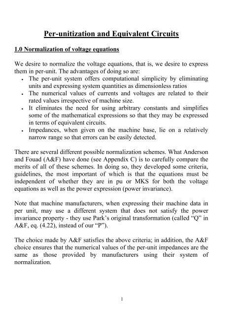
Per-unitization and Equivalent Circuits - Iowa State University

Per-unitization and Equivalent Circuits
1.0 Normalization of voltage equations
We desire to normalize the voltage equations, that is, we desire to express
them in per-unit. The advantages of doing so are:
• The per-unit system offers computational simplicity by eliminating
units and expressing system quantities as dimensionless ratios
• The numerical values of currents and voltages are related to their
rated values irrespective of machine size.
• It eliminates the need for using arbitrary constants and simplifies
some of the mathematical expressions so that they may be expressed
in terms of equivalent circuits.
• Impedances, when given on the machine base, lie on a relatively
narrow range so that errors can be easily detected.
There are several different possible normalization schemes. What Anderson
and Fouad (A&F) have done (see Appendix C) is to carefully compare the
merits of all of these schemes. In doing so, they developed some criteria,
guidelines, the most important of which is that the equations must be
independent of whether they are in pu or MKS for both the voltage
equations as well as the power expression (power invariance).
Note that machine manufacturers, when expressing their machine data in
per unit, may use a different system that does not satisfy the power
invariance property - they use Park’s original transformation (called “Q” in
A&F, eq. (4.22), instead of our “P”).
The choice made by A&F satisfies the above criteria; in addition, the A&F
choice ensures that the numerical values of the per-unit impedances are the
same as those provided by manufacturers using their system of
normalization.
1

In most undergraduate power system analyses courses, we learn that perunitization
requires selection of two base quantities out of the following
four: V, I, Z, and S, and then the base quantities for the other two are
computed. The situation is the same here, except that we also must deal
with speed (or frequency). This necessitates that we must also select a base
for either frequency (ω or f) or time, t.
In addition, we will also have need to compute base quantities associated
with flux linkage (λ) and inductance (L or M).
Our approach will be to obtain the bases for the stator side and then the
bases for the rotor side.
One may note two excellent references on the subject of per-unitizing
synchronous machine models:
1. A. Rankin, “Per-unit impedance of synchronous machines,” AIEE
Transactions, 64, Aug., 1945.
2. M. Harris, P. Lawrenson, and J. Stephenson, “Per-unit systems with
special reference to electrical machines,” Cambridge University press,
Cambridge, England, 1970.
Other references that address this subject, besides A&F, include those by
- Sauer and Pai
- Concordia
- Padiyar
- Kundur
and also course notes from de Mello.
1.1 Stator side per-unitization:
We select our stator-side bases as:
• V B : the stator rated line-neutral voltage, rms.
• S B : the stator rated per-phase power, volt-amps
• ω B : the generator rated speed, in electrical rad/sec (=ω Re =377)
2

Then we may compute bases for the following 5 quantities:
• current:
• impedance:
• time:
t B
S
I
B
=
V
X
B
1
ω
B
B
B
=
R
B
=
Z
B
V
=
I
B
B
V
=
S
2
B
= (Note we could have used
B
t B
2π
ω
= but this
would simply provide a different scaling and is therefore arbitrary). Note
that our choice of t B is the time required for the rotor to move one
electrical radian.
• Flux linkage: λ = V t (This comes from the fact that
B
B
B
dλ
Δλ
v = ≈ ⇒ Δλ
= VΔt
)
dt Δt
λB
X
B
VB
VBt
L
B
= = = =
I ω ω I I
• Inductance:
B
B
Question: How does our choice of stator base quantities affect the per-unit
values of the d- and q-axis quantities?
To answer this question, let V and I be the rms magnitudes of the a-phase
line-neutral voltage V∠α and a-phase line current I∠γ, respectively. Then
the per-unit phasors are
V
I
V u = ∠α = Vu∠α
I u = ∠γ
= Iu∠γ
V
I
B
Now let’s investigate the 0dq quantities.
B
B
B
B
B
B
3

To begin, note that the expressions for instantaneous voltages and currents
for each phase are:
v
v
v
a
b
c
=
=
=
2V
2V
2V
sin( θ + α)
sin( θ + α −120°
)
sin( θ + α + 120°
)
Use the Park’s transformation on the above to obtain:
v0
dq
⎡
=
⎢
⎢
⎢⎣
0 ⎤
3V
sinα
⎥
⎥
3V
cosα
⎥⎦
i
i
i
a
b
c
=
=
=
i0
dq
2I
sin( θ + γ )
2I
sin( θ + γ −120°
)
2I
sin( θ + γ + 120°
)
⎡
=
⎢
⎢
⎣⎢
0 ⎤
3I
sin γ ⎥
⎥
3I
cosγ
⎥⎦
(This confirms our conclusion at the end of the last set of notes that, for
balanced conditions, the 0dq quantities are constants, i.e., DC.)
Now, per-unitize by dividing by V B and I B :
⎡ ⎤
⎡ ⎤
⎢ ⎥
⎢ ⎥
⎢ 0 ⎥ ⎡ 0 ⎤ ⎢ 0 ⎥ ⎡ 0 ⎤
⎢ 3V
v
⎥ =
⎢ ⎥
0dq
= sinα
3V
sinα
⎢ 3I
u
⎢ ⎥ ⎢ ⎥
i
⎥ ⎢ ⎥
0dq
= sin γ = 3I
u
sin γ
u V
⎢ ⎥
B
u ⎢ I ⎥
B
⎢ ⎥ ⎢⎣
3V
u
cosα
3V
⎥⎦
⎢ ⎥ ⎢⎣
3I
u
cosγ
⎥⎦
⎢ cosα
⎥
3I
⎢ cosγ
⎥
⎢⎣
VB
⎥⎦
⎢⎣
I
B ⎥⎦
Observe about the above that
1. The per-unit d and q voltages are equal to the per-unit a-phase voltage
scaled by 3 sinα
and 3 cosα
, respectively.
2. The per-unit d and q currents are equal to the per-unit line current scaled
by 3 sin γ and 3 cosγ
, respectively.
4

1.2 Rotor-side per-unitization:
Recall that in system per-unitization, we must select a single power base
for the entire system, independent of the fact that some sections of the
system are magnetically coupled through transformers, i.e., we do NOT
choose different power bases for different sides of a transformer.
The same restriction applies here, where the rotor circuit is magnetically
coupled to the stator circuit, i.e., the power base selected for the stator side
must also be the power base used on the rotor side. This is S B .
In addition, we are required to select the same time (or frequency) base for
both the stator side and the rotor side. This is t B (or ω B ).
On the rotor side, we have 1 base left to choose. For transformers, we
typically choose the 1 remaining base as the voltage base (or current base)
according to the turns ratio. Here, however, we do not know a “turns ratio,”
and therefore we are left with problem of what, and how, to choose. (One
text treats the problem under the assumption that a “turns ratio” is known
between stator and rotor circuits - see the text by Padiyar, “Power System
Dynamics,” pp. 73-77.)
In making this choice, a problem results from the fact that stator power
levels are typically several times the rotor power levels. A&F give an
interesting comparison (see pg 95) of a typical stator-side per-phase power
rating of 100 MVA and field winding ratings of 250v, 1000A (250kw).
What are our choices of the one remaining rotor-side base quantity in this
case?
• Choose voltage base=rated voltage=250v, but then the current base is
I B =100E6/250=400000 amps, and per-unit values of field currents will
be very small.
• Choose current base=rated current=1000A, but then voltage base is
V B =100E6/1000=100000 volts, and per-unit values of field voltages will
be very small.
5

Analogy to transformers:
With transformers, we choose the base voltage (or current) on side 1, and
then we choose the base voltage (or current) on side 2 as that voltage that is
produced by the transformer on side 2 when the base voltage on side 1 is
applied. We did this because we wanted a per-unit circuit of the
transformer where the ideal transformer was eliminated.
Another way to think about what we do with transformers is that we select
current bases that would produce the same mutual flux between the two
windings, i.e., we choose I B1 and I B2 such that:
• I B1 produces λ 21 (the flux linkage from current I B1 in coil 1 that links coil 2),
• I B2 produces λ 12 (the flux linkage from current I B2 in coil 2 that links coil 1)
and λ 21 =λ 12 .
Note that λ 21 =M 21 I B1 and λ 12 =M 12 I B2 , where M 21 =M 21 =M is the mutual
inductance between the two transformer coils. If coil 1 creates λ 1 and of
this, only the mutual flux λ 21 links with coil 2, then the difference is the
leakage flux given by
λ L1 =λ 1 -λ 21 (eq. 1)
and illustrated in Fig. 1.
Leakage flux, λ L1
Mutual flux, λ 21
λ 1
Fig. 1: Mutual and Leakage flux
Here, each of these three fluxes are given by
λ L1 =l 1 I B1 , λ 1 =L 1 I B1 , and λ 21 =MI B1 (eq. 2)
where l 1 , L 1 , and M, are the leakage, self, and mutual inductances,
respectively. Substitution of (2) into (1) results in:
6

l 1 I B1 =L 1 I B1 - MI B1
and canceling I B1 gives:
l 1 =L 1 - M L 1 =l 1 +M
which implies that the self inductance is comprised of the leakage
inductance plus the mutual inductance.
Similar analysis results in L 2 =l 2 +M.
Back to synchronous machines:
We can apply the same concept to the synchronous machine as we applied
to the transformer above. That is,
We select the base currents for the four rotor-side windings F, D (Q, G) to
produce the same mutual flux in the air gap as produced by the stator-side
base current I B flowing in the corresponding fictitious d-axis (q-axis) coil.
We will begin by applying this idea to obtain the base current for the main
field winding.
Base-current for main field winding, approach 1:
One can visualize the above concept for the case of the relationship
between the F-winding and the d-winding, in Fig. 2.
d-winding
I B
F-winding
λ md
I FB
Fig. 2: Base currents in d and F windings
7

We see from Fig. 2 that we select I FB , the field winding base current, as
that current when flowing in the F-winding will produce a
mutual flux λ md equal to the same mutual flux that is
produced by a current I B flowing in the d-winding.
But how do we compute I FB ?
From our previous set of notes (see page 20), and also eq. 4.20 in text, we
derived
⎡
⎤
⎢ L0
0 0 0 0 0 0 ⎥
⎥
3 3
⎥
⎡λ
⎤
0 Ld
0 M
F
M
D
0 0
0
⎢
⎢
⎡i
0 ⎢
2 2
⎥
⎢
⎢
λ ⎥ ⎢
⎥
d
3 3 id
⎢ ⎥
⎢
⎢ 0 0 Lq
0 0 M
Q
M
G ⎥
⎢λ
⎥
2 2 ⎢i
q
q
⎢
⎥
⎢ ⎥
⎢
= ⎢
3
λ
⎥
⎢
F
⎥
0 M
F
0 LF
M
R
0 0 ⎢iF
⎢ 2
⎥
⎢λ
⎥
⎢
D ⎢ 3
⎥ iD
⎢ ⎥
⎢
⎢
D
R
D
⎥
⎢
λ
0 M 0 M L 0 0
Q ⎥
⎢iQ
⎢
2
⎥
⎢⎣
λ ⎥⎦
⎢
G ⎢
3
0 0 M
⎥⎣iG
Q
0 0 LQ
M
Y
⎢
2
⎥
⎢
3
⎥
⎢ 0 0 M
G
0 0 M
Y
LG
⎥
⎣
2
⎦
eq. (4.20’)
From this, we can see that
λ
d
= L
did
+ kM
FiF
+ kM
DiD
(eq. 3)
where k=√(3/2).
L d i d is all of the flux produced by the d-winding, but only a part of this flux,
the mutual flux, links with the F-winding. Call this flux from the d-winding
that links with the F-winding λ md , given by λ md =L md i d , where L md is the
mutual inductance associated with this flux (A&F call it a magnetizing
inductance).
⎤
⎥
⎥
⎥
⎥
⎥
⎥
⎥
⎥
⎥
⎦
8

As with the case of the transformer, the difference between the total flux
from the d-winding and the mutual flux is attributed to the leakage flux λ L,
so that,
l d i d =L d i d - L md i d (eq. 4)
Canceling the current i d , we see that
l d =L d -L md L d =l d +L md (eq. 5)
When I B flows in the d-winding, so that i d =I B , the mutual flux is given by
λ md =L md I B (eq. 6)
Looking back at eq (3), we see that the flux from the F-winding that links
the d-axis winding is just kM F i F .
Our criteria for selecting I FB says that when I FB flows in the F-winding, the
mutual flux linking the d-winding should equal the mutual flux from the d-
winding linking the F-winding when it carries I B . Thus, we write that
λ md =L md I B =kM F I FB (eq. 7)
And we see that
L
I = I
(eq. 8)
md
FB
B
kM
F
M F and L md are generally provided in (or can be obtained from)
manufacturer’s data for a given machine.
• M F can be computed as illustrated in Section 2.3 below, using the
magnetization curve,
• L md =L d -l d , where manufacturer’s data sheets contain L d and l d .
Therefore, once I B is selected, I FB may be computed.
Note an important point: in MKS units (i.e., henries), L md is not the same as
kM F , i.e., the reciprocal mutuals are not equal!
Base current for main field winding, approach 2:
One may also develop a relation for I FB from the perspective of the flux
linking the field winding, i.e., instead of using eq. (3) from (4.22’), use:
λ
F
= kM
Fid
+ LFiF
+ M
RiD
(eq. 9)
9

Similar to eq. (5), the self inductance L F is comprised of the leakage and
the mutual, i.e.,
L F =l f +L mF (eq. 10)
Inspecting eq. (9), we see that the flux from the d-winding linking with the
F-winding is kM F i d , so that when i d =I B and i F =I FB , we have that
L mF I FB =kM F I B (eq. 11)
and we see that
kM
L
F
I
FB
= I
B
(eq. 12)
mF
where, as before, M F is obtained per Section 2.3 below, L mF =L F -l F , and L F ,
l F are obtained from manufacturer’s data sheet.
Base current for D-winding:
We select the D-winding base current, I DB according to the following
criteria:
We select I DB , the D-winding base current, as that current when
flowing in the D-winding will produce a mutual flux λ md equal to
the same mutual flux that is produced by a current I B flowing in the
d-winding.
Similar analysis as for the F-winding results in
L
kM
I = (eq. 13)
md
D
I
DB
= I
B , DB
I
B
kM
D
LmF
We may also utilize a similar procedure between D and F windings to
obtain
L
mF
I
DB
= I
FB
(eq. 14)
M
R
10

Base current for Q-winding:
We select Q-winding base current, I QB according to the following criteria:
We select I QB , the Q-winding base current, as that current when
flowing in the Q-winding will produce a mutual flux λ mq equal to
the same mutual flux that is produced by a current I B flowing in the
q-winding.
Similar analysis as for the F-winding results in
L
I
kM
I = I (eq. 15)
mq
Q
I
QB
=
B, QB
B
kM
Q
LmQ
Base current for G-winding:
We select the G-winding base current, I GB according to the following
criteria:
We select I GB , G-winding base current, as that current when
flowing in the G-winding will produce a mutual flux λ mq equal to
the same mutual flux that is produced by a current I B flowing in the
q-winding.
Similar analysis as for the F-winding results in
L
kM
mq
G
I
GB
= I
B, I
GB
= I
B (eq. 16)
kM
G
LmG
We may also utilize a similar procedure between Q and G windings to
obtain
L
mQ
I
GB
= IQB
(eq. 17)
M
Y
11

Summary:
Eqt. (8) together with eqts. (12-17) provide the ability to develop any of the
equations given as (4.54) in the text. These equations are:
L I = L I = L I = kM I I = kM I I =
md
2
B
mF
2
FB
mD
2
DB
F
B
FB
D
B
DB
M
R
I
FB
I
DB
L I = kM I I = L I =
mq
2
B
Q
B
QB
mQ
For example, recalling (8) is Lmd
I
FB
= I
and (12) is
F
I
B
FB
= I ,
B
kM
L
F
mF
we can multiply the left-hand-sides together and the right-hand-sides
together to obtain:
2
FB
Now define the following factors:
I
k = ,
2
QB
M
L kM
I I L I = L
Y
I
QB
md F 2
2
2
=
B
⇒
mF FB md B .
kM
F
LmF
I
k = ,
I
k = ,
I
I
GB
k =
kM
B
B
B
B
F
D
Q
G
I
FB
I
DB
IQB
IGB
Because we have the same power base on all stator and rotor circuits, we
obtain:
S = V I = V I = V I = V I = V
B
Then
B
V
k = ,
B
FB
FB
V
k = ,
FB
DB
QB
GB
F
D
Q
G
VB
VB
VB
VB
Note that these k-factors may be considered to be effective turns ratios.
DB
DB
V
k = ,
QB
QB
I
V
k =
We may also derive expressions for the resistance and inductance bases.
Note our desire is to be able to compute rotor-side bases as a function of
stator-side bases. The k-factors given above will be very handy here.
GB
I
GB
12

Rotor-side resistance bases:
R
FB
≡
V
I
FB
FB
=
V
V
FB
B
I
I
B
FB
V
I
B
B
=
k
2
F
R
B
Likewise,
2
RDB
= kDRB
Rotor-side inductance bases:
, R = k R , R =
QB
2
Q
B
GB
k
2
G
R
B
L
FB
V
≡
I
Likewise,
L
DB
=
k
FB
2
D
t
FB
L
B
B
V
=
V
FB
B
I
I
QB
B
FB
VBt
I
B
2
Q
B
B
=
k
2
F
L
, L = k L , L =
B
GB
k
2
G
L
B
Rotor-stator mutuals:
Your text, pg. 95 refers to HW problem 4.18 which states that base mutuals
must be the geometric mean of the base self-inductances, i.e.,
M = L L
12 1B 2B
Thus, we have that the base for the field winding to stator winding mutual
terms is given by (see eq. 4.57 in text):
2
M = L L = L k L =
FB B FB B F B F B
Note that it is not the same as the base self inductance L FB given above.
Likewise, we get (see eq. 4.57 in text, except here we included M GB ):
M = k L , M = k L , M =
DB
D
B
QB
Q
B
k
L
GB
k
G
L
B
13

Rotor-rotor mutuals:
There are just 2 of them (see eq. 4.57 in text, except here we included
M YB ):
2 2
M
RB
= LFBLDB
= kF
LBkDLB
= kFkDLB
Likewise,
M =
YB
k
G
k
Q
L
2.3 Example 4.1, pg 97 of text
B
This is a good example that you should review carefully. The only thing
that is perhaps not too clear is the computation of M F . I will just review that
part of it here.
Computation of M F : A&F make the statement,
“From the no-load magnetization curve, the value of field current
corresponding to the rated voltage on the air-gap line is 365 A.”
The “open-circuit characteristic” or “magnetization curve” plots
• Something proportional to exciting (field) current on horizontal axis
• Something proportional to the flux on the vertical axis.
under open-circuit conditions (the a-phase winding is open). Figure 3
below illustrates.
V a
φ
λ
B
Air-gap line
Due to saturation of
the iron (a decrease in
permeability or
increase in reluctance)
for high MMF
Fig. 3
i F
F=Ni F
H=F/l
14

The air-gap line is the V a vs. i F relation that results if the iron has constant
permeability. The solid line that bends to the right is the actual
characteristic that occurs, which shows the terminal voltage falls away
from the air-gap line as the field current is raised beyond a certain point.
This falling away is caused by saturation of the ferromagnetic material,
resulting from the decrease in permeability under high flux conditions.
Figure 4 illustrates a magnetization curve for a real 13.8 kV synchronous
machine. The vertical axis is line-to-line voltage.
Fig. 4
15

What is done in Ex. 4.1 (and what is actually done in industry to obtain
M F ), is that the field current is determined corresponding to steady-state
rated open circuit terminal voltage. This voltage is V B =V LL-rated /sqrt(s). For
Ex. 4.1, this is V B =15kV/sqrt(3)=8660 volts. This is the rms voltage, but
A&F indicate that we need the corresponding peak voltage:
V peak =√2(8660)=12,247.1 volts. But why do we need the peak voltage?
Let’s consider this question.
From first page of previous notes titled “Machine Equations,” or from eq.
(4.11’) in A&F, we have
λ = L i + L i + L i + L i + L i + L i + L
a
aa
a
ab
b
But i a =i b =i c =0 under open circuit conditions.
And i D =i Q =0 under steady-state conditions. Therefore
ac
a
c
aF
aF
F
F
λ = L i + L
Recall that the g-winding models the Q-axis flux produced by the eddycurrent
effects in the rotor during the transient period. But since we are
now considering only the steady-state condition, i G =0. Therefore
λ
a
= LaFiF
(*)
Now recall from first page of previous notes titled “Machine Equations,”
or from eq. (4.16’) in A&F, that L aF =M F cosθ, and substitution into (*)
yields
λa
= M
FiF
cosθ
(**)
Differentiating (**) results in
dλ
dt
a
dθ
= −M
FiF
sinθ
= −ω
ReM
FiF
sinθ
dt
(***)
Now recall the voltage equation for the a-phase:
Substituting (***) into (#), we obtain
aD
aQ
i
v = −i
r − λ& + v
(#)
a
a
a
a
n
G
D
aQ
Q
aQ
i
G
16

v = −i
r + ω M i sinθ
+ v
a
a
a
Re
But under open circuit conditions, i a =0, i n =0 (implying v n =0) and we have
From (#*), we see that
F
F
v = ω M i sinθ
(#*)
a
Re
Vpeak
V
peak
= ωReM
FiF
⇒ M
F
=
i ω
So we choose a point off the magnetization curve, for example, A&F
choose i F =365 A, V peak =12,247.1 volts (365 A is the value of field current
corresponding to the rated voltage on the air-gap line, and
12,247.1/sqrt(2)=8660 volts is the rated RMS line-to-neutral voltage
(corresponding to 8660sqrt(3)=15kV). Then
M
F
V
=
i ω
Re
F
peak
And from this we can compute
F
F
F
n
Re
12,247.1
−3
= = 89.006×
10
(365)(377)
k
F
kM
=
L
md
F
=
kM
F
L − l
d
d
henries
where the denominator is comprised of data provided by the manufacturer.
The rest of Ex. 4.1 is just an application of our per-unitization formula.
There is an interesting paragraph in Appendix C, pg. 552 of your text, to
which I want to draw your attention. It says,
“Note that a key element in determining the factor k F , and hence all the
rotor base quantities, is the value of M F (in H). This is obtained from the
air gap line of the magnetization curve provided by the manufacturer.
Unfortunately, no such data is given for any of the amortisseur circuits.
Thus, while the pu values of the various amortisseur elements can be
determined, their corresponding MKS data are not known.
I provide some comments on certain sentences in this paragraph:
17

• “Note that a key element in determining the factor k F , and hence all the
rotor base quantities,” refers to the fact that we obtain L FB and R FB
from:
L
R
FB
FB
= k
= k
2
F
2
F
L
B
R
B
• “This is obtained from the air gap line of the magnetization curve
provided by the manufacturer,” as we have seen above by using
V
M
F
=
i
peak
Fω Re
We are able to get M F in this way because we can directly control the
current i F , with no other circuits energized (as a result of the opencircuit,
steady-state conditions), and directly measure the induced
voltage at the a-phase terminals.
• “Unfortunately, no such data is given for any of the amortisseur
circuits.” It is not possible to directly control the currents i D , i Q , and i G ,
since their corresponding circuits do not have sources. The only way to
energize these circuits is via a transient condition, but there is no way to
provide a transient condition that will also not energize other circuits,
which would result in the measured terminal voltage being induced
from the mutual inductance between itself and the other circuits as well.
• “Thus, while the pu values of the various amortisseur elements can be
determined, their corresponding MKS data are not known.” In example
4.1, the text puts an asterisk by some of the parameters (L D , L Q , kM D ,
kM Q , r D , and r Q ), indicating they were “estimated for academic study”).
This is because manufacturer’s datasheets do not always include the
parameters for the amortisseur (and g-winding) circuits, simply because
they are hard to measure (based on the comments of the previous
bullet). However, it is possible to obtain the per-unit value (not the
MKS value) of some of the amortisseur circuit parameters (specifically,
the mutual inductances), because, as we shall see in Section 3.0 below,
in per-unit, all direct-axis rotor mutuals are equal and all quadratureaxis
mutuals are equal! In other words:
18

• D-axis mutuals:
F-d winding mutual, kM F
D-d winding mutual, kM D
F-D winding mutual, M R (can be called M X in some texts)
That is, we will show that in per-unit, kM
Fu
= kM
Du
= M
Ru
• Q-axis mutuals:
G-q winding mutual, kM G
Q-q winding mutual, kM Q
G-Q winding mutual, M Y
That is, we will show that in per-unit, kM
Qu
= kM
Gu
= M
Yu
2.4 Applying the bases to voltage equations:
Recall our voltage equation as written in MKS units:
⎡
⎢
⎢
vd
⎢ vq
⎢
⎢−
v
0
⎢
⎢
⎢
⎢
⎣
v
0
0
0
⎤ ⎢
⎥ ⎢
⎥ ⎢
⎥ ⎢
⎥ ⎢
⎥ = −⎢
⎥
F
⎥
⎥
⎥
⎦
⎡r
+ 3r
⎢
⎢
⎢
⎢
⎢
⎣
a
0
0
0
0
0
0
n
⎡
⎢L0
+ 3L
⎢
⎢
⎢
0
⎢
⎢ 0
⎢
⎢
− ⎢ 0
⎢
⎢
⎢ 0
⎢
⎢
⎢ 0
⎢
⎢ 0
⎢⎣
n
0
r
b
−ωL
0
0
0
0
D
0
L
d
0
3
M
2
3
M
2
0
0
ωL
F
D
0
r
c
0
0
0
0
q
3
−ω
M
2
r
0
0
L
q
0
0
3
M
2
3
M
2
Q
G
0
0
F
0
0
0
F
0
3
M
2
0
L
M
−ω
F
0
0
R
F
0
0
3
M
2
0
r
D
0
0
L
D
0
3
M
2
0
M
R
D
0
0
0
3
ω M
2
D
0
0
0
r
Q
0
0
0
L
M
Q
3
M
2
0
0
Q
Y
Q
0
3
ω M
2
0
0
0
0
r
G
0
0
M
L
Y
G
G
3
M
2
0
0
⎤
⎥⎡i
⎥⎢
⎢
i
⎥
⎥⎢i
⎥⎢
⎥⎢i
⎥⎢i
⎥⎢
⎥⎢i
⎥⎢
⎥⎣i
⎦
G
0
d
q
F
D
Q
G
⎤
⎥
⎥
⎥
⎥
⎥
⎥
⎥
⎥
⎥
⎦
⎤
⎥
⎥
⎥
⎥⎡i& 0
⎤
⎥⎢
⎥
⎥⎢i
&
d ⎥
⎥⎢i&
⎥
q
⎥⎢
⎥
⎥⎢i&
⎥
F
⎥⎢
⎥
⎥⎢i
&
D ⎥
⎥⎢
i&
⎥
⎥⎢
Q
⎥
⎥⎢
⎥
⎣i
&
G ⎦
⎥
⎥
⎥
⎥⎦
19

Let’s normalize them using our chosen bases to obtain the equations in perunit.
The per-unit equations should appear as above when done, except that
everything must be in per-unit.
Step 1: Replace all MKS voltages on the left with
• the product of their per-unit value and their base value (use V B
for the first 3 equations and V FB , V DB , V QB , V GB for the last four
equations),
and replace all currents on the right with
• the product of their per-unit value and their base value (use I B
for the first 3 equations and I FB , I DB , I QB , I GB for the last four
equations).
This results in a relation similar to eq. 4.60 in the text, as follows….
⎡ v0uVB
⎢
⎢
vduVB
⎢ vquVB
⎢
⎢−
vFuV
⎢ 0
⎢
⎢ 0
⎢
⎣
0
FB
⎤ ⎢
⎥ ⎢
⎥ ⎢
⎥ ⎢
⎥ ⎢
⎥ = −⎢
⎥
⎥
⎥
⎥
⎦
⎡r
+ 3r
⎢
⎢
⎢
⎢
⎢
⎣
a
0
0
0
0
0
0
⎡
⎢L0
+ 3L
⎢
⎢
⎢
0
⎢
⎢ 0
⎢
⎢
− ⎢ 0
⎢
⎢
⎢ 0
⎢
⎢
⎢ 0
⎢
⎢ 0
⎢⎣
n
n
−ωL
L
r
0
d
0
b
3
M
2
3
M
2
0
0
0
0
0
0
0
D
F
D
0
ωL
r
c
0
0
0
0
q
0
0
L
q
0
0
3
M
2
3
M
2
3
−ω
M
2
r
Q
G
0
0
F
0
0
0
0
L
M
F
F
3
M
2
0
0
0
R
F
− ω
(eq. 4.60’)
0
0
3
M
2
0
r
D
0
0
0
3
M
2
0
M
L
R
D
0
0
D
D
0
3
ω M
2
L
M
r
0
0
Q
Q
3
M
2
0
0
0
0
0
0
Y
Q
Q
0 ⎤
⎥⎡
i0u
I
3
ω M ⎢
G
⎥
⎢
iduI
2 ⎥
⎥⎢
iquI
0 ⎥⎢
⎥⎢iFuI
0 ⎥⎢iDuI
0 ⎥⎢
⎥⎢iQuI
0 ⎥⎢
⎥⎣iGuI
rG
⎦
0
0
3
M
2
0
0
M
L
Y
G
G
⎤
⎥
⎥
⎥
⎥⎡
i& 0 uI
⎥⎢
⎥⎢
i&
duI
⎥⎢
i&
quI
⎥⎢
⎥⎢i&
FuI
⎥⎢
⎥⎢i
&
DuI
⎥⎢
i&
⎥⎢
QuI
⎥⎢
⎣i
&
GuI
⎥
⎥
⎥
⎥⎦
B
B
B
FB
DB
QB
GB
B
B
B
FB
DB
QB
GB
⎤
⎥
⎥
⎥
⎥
⎥
⎥
⎥
⎥
⎥
⎥
⎦
⎤
⎥
⎥
⎥
⎥
⎥
⎥
⎥
⎥
⎥
⎦
20

Step2: For each of the equations in the above, we need to divide through by
the voltage base. For those equations containing ω, we replace it with
ω=ω u ω B (ω B =ω Re ). Then we do some algebra-work on each equation to
express the coefficients of each current and current derivative as perunitized
self or mutual inductances. As an example, the second equation is
done for you in the text; here, I will do the last equation, corresponding to
the G-winding….
0( V
GB
) = −r
G
i
Gu
I
GB
−
3
M
2
Step 2a: Divide through by V GB to obtain:
− rG
0 =
VGB
I
GB
i
Gu
−
3
2
G
i&
M
V
I
qu
GB
B
G
I
B
i&
qu
− M
Y
M
−
V
I
GB
QB
i&
Y
Qu
i&
I
Qu
QB
−
L
−
V
I
The first term has a denominator of R GB . The last three terms are not so
obvious. We desire them to have denominators of M GB , M YB , and L GB ,
2
respectively, where, from above, we recall k L k k L L = k L ,
where
V
k =
GB B
G
= , and
VB
I
GB
I
I
B
k
Q
= .
I
QB
G
GB
L
GB
G
i&
i&
Gu
M
GB
=
G B
,
YB G Q B
Gu
I
GB
M = ,
GB G B
Step 2b: Let’s multiply the denominator of the last three terms by V B /V B .
This results in:
− r
0 =
R
G
GB
i
Gu
−
3
2
M
G
VGB
V
V I
B
B
B
i&
qu
M
Y
−
VGB
V
V I
B
B
QB
i&
Qu
LG
−
VGB
V
V I
Step 2c: Let’s multiply the denominator of the last two terms by I B /I B . This
results in:
B
B
GB
i&
Gu
21

0
=
− r
R
G
GB
i
Gu
−
3
2
M
G
V V
V
GB
B
I
B
B
i&
qu
−
V
V
GB
B
M
V
I
B
B
Y
I
I
B
QB
i&
Qu
−
V
V
GB
B
L
V
I
G
B
B
I
I
B
GB
i&
Gu
VGB
I
B
Step 2d: Recall the k-factors (pg 96 of text): k
G
= = , and
VB
I
GB
Substitution yields:
− rG
3 M
G
M
Y
LG
0 = iGu
− i&
qu
− i&
Qu
− i&
Gu
RGB
2 VB
VB
2 VB
kG
kGkQ
kG
I
I I
B
B
B
I
B
k
Q
= .
I
QB
Step 2e: We are close now, as we need M GB =k G L B , M YB =k G k Q L B , and
L GB =(k G ) 2 L B , respectively, on the denominator of the last three terms.
Recall that L B =V B /(ω B I B ), so we need to divide top and bottom on the
denominators of the last three terms by ω B . Doing so yields:
− r
i
3
2
M
G
G
Y
0 =
Gu
−
qu
−
Qu
−
R
VB
V
GB
B
kG
ω
B
kGkQ
ω
B
ω
B
I
B
ω
B
I
B
Step 2f: And substituting in L B results in:
i&
M
i&
k
2
G
L
V
B
G
B
ω I
B
ω
B
i&
Gu
− r
i
3
2
M
0 G
G
Y
=
Gu
−
qu
−
Qu
RGB
kG
LBω
B
kGkQLBω
−
B
i&
M
i&
k
2
G
L
L
G
B
ω
B
i&
Gu
Step 2g: Recalling that M GB =k G L B , M YB =k G k Q L B , and L GB =(k G ) 2 L B , we
may write:
0 =
− r
R
G
GB
i
Gu
which results in
−
3
2
M
M
GB
G
ω
B
i&
qu
−
M
M
YB
Y
ω
B
i&
Qu
−
L
L
GB
G
ω
B
i&
Gu
22

0
= −r
Gu
i
Gu
−
3
2
M
ω
Gu
B
i&
qu
−
M
ω
Yu
B
i&
Qu
−
L
ω
Gu
B
i&
Gu
Step 2h: However, we still have one problem. Recall that we want the
equations to be identical in pu to their form in MKS units. But in the last
equation, we still have ω B , which does not appear in our MKS equation.
We can take care of it, however, by recalling that ω B =1/t B , so that:
1
i&
ω
B
1
i&
ω
B
1
i&
ω
B
qu
Qu
Gu
=
=
=
1
1
t
B
1
1
t
B
1
1
t
B
diqu
diqu
=
dt
d⎜
⎛ t
⎝ tB
diQu
diQu
=
dt
d⎜
⎛ t
⎝ tB
diGu
diGu
=
dt
d⎜
⎛ t
⎝ t
where τ=t/t B is the normalized time.
⎟
⎞
⎠
B
⎟
⎞
⎠
diqu
= ;
dτ
⎞
⎟
⎠
diQu
= ;
dτ
diGu
=
dτ
With this last change, we can write, finally, that
0 = −r
G
i
Gu
−
3
2
which is the per-unitized form of the last equation in eq. (4.60’).
M
Gu
Note that it is exactly the same form as the original equation in MKS units.
i&
Similar work can be done for the other equations, resulting in equations
similar to eq. 4.74 in your text:
qu
−
M
Yu
i&
Qu
−
L
Gu
i&
Gu
23

⎡ vd
⎢
− v
⎢
⎢ 0
⎢
⎢
vq
⎢ 0
⎢
⎣ 0
F
⎤ ⎡ r 0
⎥ ⎢
0 rF
⎥ ⎢
⎥ ⎢ 0 0
⎥ = −⎢
⎥ ⎢
−ωLd
−ωkM
F
⎥ ⎢ 0 0
⎥ ⎢
⎦ ⎣ 0 0
⎡ Ld
kM
F
kM
⎢
kM
F
LF
M
⎢
⎢kM
D
M
R
L
− ⎢
⎢
0 0 0
⎢ 0 0 0
⎢
⎣ 0 0 0
(eq. 4.74’)
D
R
D
r
D
−ωkM
L
0
0
0
0
0
0
0
q
kM
kM
Q
G
D
0
0
r
0
0
0
0
0
kM
ωL
L
M
Q
Y
Q
q
ωkM
0
0
0
kM
M
L
Y
G
0
0
0
r
G
Q
0
Q
⎤⎡i&
⎥⎢
i&
⎥⎢
⎥⎢i&
⎥⎢
⎥⎢
i&
⎥⎢i&
⎥⎢
⎦⎣i&
d
F
D
q
Q
G
ωkM
⎤
⎥
⎥
⎥
⎥
⎥
⎥
⎥
⎦
0
0
0
0
r
G
G
⎤⎡i
⎥⎢
i
⎥⎢
⎥⎢i
⎥⎢
⎥⎢
i
⎥⎢i
⎥⎢
⎦⎣i
d
F
D
q
Q
G
⎤
⎥
⎥
⎥
⎥
⎥
⎥
⎥
⎦
Note that in the above equation,
• The “u” subscript was dropped; however, all parameters are in
per-unit.
• We have dropped the zero-sequence voltage equation since we
will be interested in balanced conditions for stability studies. (A
system having a three-phase fault, considered to be, usually, the
most severe, is still a balanced system. This does not mean that
we cannot analyze unbalanced faults using stability programs. It
is possible to analyze the effects of unbalanced faults on the
positive sequence network represented in stability programs –
see Kimbark Vol I, pp. 220-221). Otherwise, eq. (4.74’) is
precisely the same as eqt. 4.39 in your text (see the same
24

equation as 4.39, except for the “G” winding included, on page
27 of the notes called “macheqts”– we called it there, eq. 4.39’).
• The equations are rearranged to better display the coupling and
decoupling between the various circuits. This coupling can be
well illustrated by a figure similar to Fig. 4.3 in your text, given
below as Fig. 4.3’. Notice that the coupling between the F and D
windings is captured by M X . We have called this mutual
inductance M R in our work above to remain consistent with
A&F.
r 0
+3r n i 0
+
L 0
+3L n
v 0
r F
-
vD =0
-
i F
+
-
L F
•
+
L D
r D
r a i d
kM F
+
M X
L v d d
i •
D •
-
kM D
-
ωλ q
+
r G
v G =0
v Q =0
+
-
+
-
r Q
i G •
L G
L Q
M Y
kM G
•
kM Q
L q
•
r a
+ -
ωλ d
+
v q
-
Fig 4.3’
25

Now let’s make some definitions:
⎡r
0
⎢
⎢
0 rF
⎢0
0
R = ⎢
⎢0
0
⎢0
0
⎢
⎢⎣
0 0
⎡ Ld
⎢
⎢
kM
F
⎢kM
D
L = ⎢
⎢ 0
⎢ 0
⎢
⎢⎣
0
⎡ vd
⎢
⎢
− v
⎢ 0
v = ⎢
⎢ vq
⎢ 0
⎢
⎣ 0
F
r
⎤
⎥
⎥
⎥
⎥;
⎥
⎥
⎥
⎦
0
0
D
0
0
0
kM
L
M
F
0
0
0
R
F
0
0
0
r
0
0
0
0
0
0
r
Q
0
kM
M
L
R
D
0
0
0
D
0 ⎤
0
⎥
⎥
0 ⎥
⎥ ;
0 ⎥
0 ⎥
⎥
rG
⎥⎦
0
0
0
L
q
kM
kM
Q
G
⎡id
⎤
⎢ ⎥
⎢
iF
⎥
⎢i
⎥
D
i = ⎢ ⎥
⎢iq
⎥
⎢i
⎥
Q
⎢ ⎥
⎢⎣
iG
⎥⎦
⎡ 0
⎢
⎢
0
⎢ 0
N = ⎢
⎢−
L
⎢ 0
⎢
⎣ 0
0 0
0
0
kM
L
M
Q
Y
Q
0
0
kM
M
L
Y
G
d
G
⎤
⎥
⎥
⎥
⎥
⎥
⎥
⎥
⎥⎦
0
0
0
− kM
0
0
F
0
0
0
− kM
0
0
D
L
q
0
0
0
0
0
kM
0
0
0
0
0
Q
kM
0
0
0
0
0
G
⎤
⎥
⎥
⎥
⎥
⎥
⎥
⎥
⎦
With these definitions, we rewrite eqt. (4.74’) in compact notation:
v = −( R + ω N)
i − Li&
(eq. 4.75)
We may solve eq. (4.75) for di/dt so that it is in state-space form:
−1
−1
&
(eq. 4.76)
i
= −L
( R + ω N ) i −
L
v
26

3.0 Per-unit mutuals (See Section 4.11)
A useful observation regarding per-unit values of M F , M D , and M R :
Recall our definitions of the D-axis k-factors:
I
B
V
k
F
= =
I
FB
V
I
B
V
k
D
= =
I V
FB
B
DB
DB B
and that we developed (see eqs. 4.54, pg 12-13 of these notes):
2 2
2
L
md
I
B
= LmF
I
FB
= LmD
I
DB
= kM
F
I
BI
FB
= kM
DI
BI
DB
= M
RI
FB
I (17)
DB
1 2 3 4 5 6
From the first and fourth expression in eq (17), we have:
L I = kM
md
Thus,
2
B
F
I
B
I
FB
I
I
B
FB
kM
F
= (18)
Lmd
Likewise, from the first and fifth, and from the fourth and sixth
expressions in eq (17), we have:
L I =
md
Thus,
2
B
kM
I
D
I
B
I
DB
kM
kM I I =
B D
B R
= and = (19)
I
DB
Lmd
I
DB
kM
F
From the definitions of the k-factors, and eqs (18) and (19), we
have:
kM
L
F
k
F
= and
md
F
I
B
FB
M
kM
k =
M
M
R
I
FB
I
DB
D R
D
= (20)
Lmd
kM
F
27

Also, from eq. 4.57 in text (also see p13-14 of these notes), we find
M
FB
= kF
LB, DB D B
M = k L , M
RB
= kFkDL
(21)
B
which we got by using the fact that base mutuals must be the
geometric mean of the base self-inductances (see prob 4.18).
Now, recall the elements in the per-unitized voltage equations as
given by eq. 4.74’ (see page 24 of these notes).
⎡ vd
⎤ ⎡ r 0 0 ωLq
ωkM
Q
ωkM
G ⎤⎡id
⎢ ⎥ ⎢
⎥⎢
⎢
− vF
⎥ ⎢
0 rF
0 0 0 0
⎥⎢
iF
⎢ 0 ⎥ ⎢ 0 0 r
⎥⎢
D
0 0 0 iD
⎢ ⎥ = ⎢
⎥⎢
⎢ vq
⎥ ⎢−ωLd
−ωkM
F
−ωkM
D
r 0 0 ⎥⎢iq
⎢ 0 ⎥ ⎢ 0 0 0 0 r ⎥⎢
Q
0 iQ
⎢ ⎥ ⎢
⎥⎢
⎣ 0
⎦ ⎢⎣
0 0 0 0 0 rG
⎥⎦
⎢⎣
iG
⎡ Ld
kM
F
kM
D
0 0 0 ⎤⎡i&
d
⎤
⎢
⎥⎢
⎥
⎢
kM
F
LF
M
R
0 0 0
⎥⎢
i&
F ⎥
⎢kM
⎥⎢
⎥
D
M
R
LD
0 0 0 i&
D
− ⎢
⎥⎢
⎥
⎢ 0 0 0 Lq
kM
Q
kM
G ⎥⎢i
&
q ⎥
⎢ 0 0 0 kM
⎥⎢
⎥
Q
LQ
M
Y i&
Q
⎢
⎥⎢
⎥
⎢⎣
0 0 0 kM
G
M
Y
LG
⎥⎦
⎢⎣
i&
G ⎥⎦
4.74’
In particular, consider the mutual terms in the last matrix for the d-
axis. This would be the upper left-hand 3x3 block. These terms, in
pu, are by definition the ratio of the term in MKS to the
appropriate base. Therefore:
• Stator-field mutual:
kM
M
F
kM
Fu
= .
FB
Substituting for M FB from eq. (21) and then k F from eq. (20)
results in:
⎤
⎥
⎥
⎥
⎥
⎥
⎥
⎥
⎥⎦
28

kM
Fu
=
kM
M
F
FB
=
kM
k L
F
F
B
=
kM
kM
F
F
L
L
md
B
=
L
L
md
B
≡
L
mdu
kM
M
• Stator-D-winding damper mutual: kM
Du
=
D
.
DB
Substituting for M DB from eq. (21) and then k D from eq. (20)
results in:
kM
Du
=
kM
M
D
DB
=
kM
k L
D
D
B
=
kM
kM
• Field-D-winding damper mutual:
M
Ru
D
D
L
L
Ru
md
B
M =
=
L
L
M
M
md
R
B
≡
L
mdu
RB
Substituting for M RB from eq. (21) and then k F and k D from
eq. (20) (using the 2 nd expression for k D in eq. (4)) results in:
M
=
M
R
RB
=
k
F
M
k
D
R
L
B
M
RLmd
kM
=
kM M L
Important fact: In per-unit, all d-axis mutuals are numerically
equal! We will define a new term for them, L AD , as the per-unit
value of any d-axis mutual inductance, so that:
L ≡ L = kM = kM =
AD mdu Fu Du Ru
Also note that, since the mutual is the difference between the self
and the leakage, this implies
L du -l du =L Du -l Du =L Fu -l Fu =L AD
The above relations are given in eqs. 4.107 and 4.108 in your text.
F
R
F
B
=
L
L
M
md
B
≡
L
mdu
29

We can go through a similar process for the q-axis mutuals (from
4.74’, we see that these are the terms in the lower right-hand block
of the matrix, kM Q , kM G , and M Y ). I will leave this for you to do.
The result is:
L ≡ L = kM = kM =
AQ mqu Qu Gu Yu
L qu -l qu =L Qu -l Qu =L Gu -l Gu =L AQ
The above relations are given by eq. 4.109 in your text, except for
the addition of the G-term and the Y-term.
L AD and L AQ are very important for drawing the equivalent circuits.
They are also important in dealing with saturation because they
provide for the definition of the per-unit mutual flux (we will see
this in our development of the flux-linkage state-space model).
4.0 Equivalent Circuits (See Section 4.11)
Let’s return to the voltage equations that we had before we folded
in the speed voltage terms. They were:
M
⎡ v0
⎤ ⎡ra
⎢ ⎢
⎢
vd
⎢0
⎢ v ⎢
q 0
⎢ ⎢
⎢−
vF
= −⎢0
⎢ 0 ⎢
⎢ ⎢
⎢ ⎥ ⎥⎥⎥⎥⎥⎥⎥ 0
0 ⎢0
⎢ ⎥ ⎢
⎣
0
⎦ ⎣0
⎡ 0 ⎤ ⎡3r
i0
− 3L i&
n n 0⎤
⎢ ⎥ ⎢ ⎥
⎢
−ωλq
⎢ 0
⎥
⎥
⎢ ωλ ⎥ ⎢ ⎥
d
0
⎢ ⎥ ⎢ ⎥
+ ⎢ 0 ⎥ + ⎢ 0 ⎥
⎢ 0 ⎥ ⎢ 0 ⎥
⎢ ⎥ ⎢ ⎥
⎢ 0 ⎥ ⎢ 0 ⎥
⎢ ⎥ ⎢ ⎥
⎣ 0 ⎦ ⎣ 0 ⎦
r
0
0
0
0
0
0
b
0
0
0
0
0
r
0
c
r
0
0
0
0
0
0
F
r
0
0
0
0
0
0
D
0
0
0
0
0
r
0
Q
⎡
⎢
⎢
⎢
0⎤⎡i
⎢
0 ⎤
⎥⎢
⎥ ⎢
0⎥⎢
id
⎥ ⎢
0⎥⎢i
⎥ ⎢
q
⎥⎢
⎥ ⎢
0⎥⎢iF
⎥ − ⎢
⎢ ⎥ ⎢
0⎥
iD
⎥⎢
⎥ ⎢
0⎥⎢i
⎥ ⎢
Q
⎥⎢
⎥ ⎢
rG
⎦⎣iG
⎦ ⎢
⎢
⎢
⎢
⎢⎣
L
0
0
0
0
0
0
0
0
L
d
0
3
M
2
3
M
2
0
0
F
D
0
0
L
q
0
0
3
M
2
3
M
2
Q
G
0
3
M
2
0
L
M
F
R
0
0
F
0
3
M
2
0
M
L
R
D
0
0
D
0
0
3
M
2
0
0
L
M
Q
Y
Q
0
0
3
M
2
0
0
M
L
Y
G
⎤
⎥
⎥
⎥
⎥⎡i
&
0
⎤
⎥⎢
⎥
⎥⎢i
&
d ⎥
⎥⎢i&
⎥
q
⎥⎢
⎥
⎥⎢i&
⎥
F
⎥⎢
⎥
⎥⎢i
&
D ⎥
⎥⎢
⎥
⎥⎢
i&
Q
⎥
⎥⎢
⎥
⎣i
&
G ⎦
⎥
⎥
⎥
⎥⎦
G
30

Assume all of the above is in per-unit (but we have dropped the u-
subscript).
There is some advantage to re-writing these equations in terms of
L AD and L AQ. For example, consider the d-axis equation. It is:
v
d
= −ri
− L i&
− kM i&
− kM i&
d
d
d
F
F
D
D
−ωλ
q
Recall that L d =L md +l d L md =L d -l d
Let’s modify the d-axis voltage equation by adding and subtracting
l d (di d /dt) :
v
d
= −ri
− L i&
+ l i&
− l i&
− kM i&
− kM i&
d
d
d
d
d
d
d
F
F
D
D
−ωλ
which can be written as:
v = −ri
− l i&
−[( L − l ) i&
+ kM i&
+ kM i&
] −ωλ
d
d
d
d
d
d
d
The advantage to this is that, in per-unit, we recall that L d -
l d =kM F =kM D ≡L AD . Therefore,
v = −ri
− l i&
− L [ i&
+ i&
+ i&
] −ωλ
d
d
d
d
AD
d
F
D
Let’s repeat this for the G-axis equation, which is, from the matrix
equation at the beginning of this section:
v
G
= 0 = −r
G
i
G
− kM
G
i&
q
− M
Y
i&
Q
F
F
q
− L
Let’s modify the G-winding voltage equation by adding and
subtracting l G (di G /dt) :
v
G
= 0 = −r
G
i
G
− kM
G
i&
q
− M
Y
i&
Q
− L
G
i&
G
G
i&
G
+ l
which can be written as:
v = 0 = −r
i − kM i&
− M i&
− ( L − l ) i&
G
G
G
G
q
Y
Q
The advantage to this is that, in pu, we have L G -l G =kM G =M Y ≡L AQ .
G
G
G
D
i&
G
G
D
− l
− l
G
G
i&
i&
G
G
q
q ,
31

Therefore
v
G
= 0 = −rG
iG
− lGi& G
− LAQ
( i&
q
+ i&
Q
+ i&
G
)
Repeating this procedure for the F, D, and q equations, and then
summarizing, we obtain:
D-axis relations:
v = −ri
− l i&
− L [ i&
+ i&
+ i&
] −
d
− v
v
D
F
=
d
= −r
i
d
d
− l
AD
d
F
D
ωλ
i& [ ]
F
− LAD
i&
d
+ i&
F
+ i&
D
i& − L [ i&
+ i&
+ i&
]
F F F
0 = −rDiD
− lD
D AD d F D
Q-axis relations:
v = −ri
− l i&
− L ( i&
+ i&
+ i&
) +
v
v
q
Q
G
q
q
q
AQ
q
Q
G
ωλ
= 0 = −riQ
− lQi& Q
− LAQ
( i&
q
+ i&
Q
+ i&
G
)
= = −r
i − l i& − L ( i&
+ i&
+ i&
)
0
G G G G AQ q Q G
We desire to draw circuits that are characterized by these
equations.
Note:
• The D-axis relations are coupled through the L AD terms.
• This term, for each equation, may be represented by a single
“center” branch.
• The other terms, for each equation, may be represented as
single branches which feed the center branch.
This results in the circuit of Fig 4.5 in your text.
Similar reasoning results in the circuit of Fig. 4.6 in your text.
We redraw these circuits below.
q
d
32

v
d
= −ri
− l i&
− L [ i&
+ i&
+ i&
] −ωλ
d
d
d
AD
− v
[ ]
F
= −rF
iF
− lFi& F
− LAD
i&
d
+ i&
F
+ i&
D
v = = −r
i − l i& − L [ i&
+ i&
+ i&
]
D
0
D D D D AD d F D
d
F
D
q
l d
i d
r
l F
l D
r F
i F
r D
i D
L AD
i F +i D +i d
v d
v F
-
+
-- +
ωλ q
Direct-axis equivalent circuit:
The above is the same as Fig. 4.5 in your text
v
v
v
q
Q
G
= −ri
− l i&
− L ( i&
+ i&
+ i&
) + ωλ
q
q
q
AQ
= 0 = −riQ
− lQi& Q
− LAQ
( i&
q
+ i&
Q
+ i&
G
)
= = −r
i − l i& − L ( i&
+ i&
+ i&
)
0
G G G G AQ q Q G
q
Q
G
d
l q
i d
r
l G
l Q
r G
i G
r Q
i Q
L AQ
i Q +i G +i q
v q
-- +
Quadrature-axis equivalent circuit:
The above is the same as Fig. 4.6 in your text, except we have
included the G-circuit
ωλ d
33

The ability to draw these circuits is a direct result of the L AD and
L AQ relations that occur only in per-unit. Therefore, it is important
to be in the per-unit system when utilizing these circuits.
These equivalent circuits are useful for:
• Remembering the voltage relations
• Gaining physical understanding of relations between d-q-F-D-
Q-G quantities.
• Reading the literature, where you will see them often.
34