FLUTE Based Obstacle-Avoiding Rectilinear Steiner Tree Construction

1
ISPD: FOARS: FLUTE Based Obstacle-Avoiding
Rectilinear Steiner Tree Construction
Gaurav Ajwani, Student Member, IEEE, Chris Chu, Senior Member, IEEE, and Wai-Kei Mak, Member, IEEE
Abstract—In this paper, we present an algorithm called FOARS
for obstacle-avoiding rectilinear Steiner minimal tree (OARSMT)
construction. FOARS applies a top-down approach which first
partitions the set of pins into several subsets uncluttered by
obstacles. Then an obstacle-avoiding Steiner tree is generated
for each subset by an obstacle aware version of the rectilinear
Steiner minimal tree (RSMT) algorithm FLUTE. Finally, the
trees are merged and refined to form the OARSMT. To guide the
partitioning of pins, we propose a novel algorithm to construct
a linear-sized obstacle-avoiding spanning graph (OASG) which
guarantees to contain a rectilinear minimum spanning tree if
there is no obstacle. Experimental results show that FOARS
is among the best algorithms in terms of both wirelength and
runtime for testcases both with and without obstacles.
Index Terms—Physical Design, Routing, Spanning Graph,
RSMT
I. INTRODUCTION
With the advent of re-usability using Intellectual Property
(IP) sharing, the chip in today’s design is completely packed
with fixed blocks such as IP blocks, macros, etc. Routing of
multi-terminal nets in the presence of obstacles has become
a quintessential part of the design and has been studied by
many (e.g., [1]–[13]). As pointed out by Hwang [14], in the
absence of obstacles multi-terminal net routing corresponds to
the rectilinear Steiner minimal tree (RSMT) problem which is
NP-complete. The presence of obstacles in the region makes
multi-terminal routing problem even harder.
In this work, we develop a new algorithm called FOARS for
OARSMT and RSMT generation by leveraging FLUTE [15].
FLUTE is a very fast and robust tool for RSMT generation.
It is widely used in many recent academic physical design
tools. FLUTE by its design cannot handle obstacles. A simple
strategy to generate an OARSMT would be to call FLUTE
once and legalize the edges intersecting with obstacles. Unfortunately,
the OARSMT obtained can be far from optimal as
its topology is based on an obstacle-oblivious Steiner tree. A
better strategy is to break the RSMT produced by FLUTE on
edges overlapping with obstacles, recursively call FLUTE to
locally optimize the subtrees, and then combine all overlapfree
subtrees at the end. However, if the routing region is
severely cluttered with obstacles, the quality of the solution
produced will degrade because the RSMTs generated by
FLUTE may be excessively broken. To tackle this, we propose
a partitioning algorithm with a global view of the problem at
the top level to divide the problem into smaller uncluttered
instances. Even if there is no obstacle, when the number of
pins are more than several tens, the partitioning algorithm
can improve both the wirelength and runtime of FLUTE as it
works better than the greedy net breaking heuristics in FLUTE.
To guide the partitioning algorithm, we propose to use
a sparse spanning graph. In the presence of obstacles, this
graph will be an obstacle-avoiding spanning graph (OASG).
An OASG is used to capture the proximity information among
the pins and corners of obstacles, if any. Three categories of
graph were used to capture the proximity information during
OARSMT construction in the past. [1], [3], [4], [10] all use
the escape graph. [9] utilizes a Delaunay triangulation based
graph. Both the escape graph and Delaunay triangulation based
graph contain O(n 2 ) edges, where n is the total number of
pins and obstacle corners. [2], [5]–[8] are based on various
forms of obstacle-avoiding spanning graphs. Shen et al. [2]
proposed a form of OASG that only contains a linear number
of edges which is also adopted in [5]. Later Lin et al. [6]
proposed adding missing “essential edges” to Shen’s OASG.
Unfortunately, it increases the number of edges to O(n 2 )
in the worst case (O(n log n) in practice) and hence the
time complexity of later steps of OARSMT construction is
increased to a large extent. In view of that, Long et al. [7],
[8] proposed a quadrant approach to generate an OASG with
a linear number of edges. But as we will see later, the OASG
generated by Long’s approach is not ideal. In this paper, we
present a novel octant approach to generate an O(n)-edge
OASG with more desirable properties.
Different from [2], [6]–[8] which directly use an OASG to
construct an OARSMT, we only use an OASG to guide the
partitioning and construct our final OARSMT using FLUTE.
We note that a shortcoming of the former approach is that the
resulting OARSMT tends to follow obstacle boundaries and
makes detours towards obstacle corners. This makes it easier
to lead to congestion when routing many nets in a design.
(Adding essential edges as in [6] will help but will result in
O(n 2 ) edges as an escape graph.) On the other hand, since
we only utilize the OASG to guide our partitioning and use
FLUTE for local optimization, the OARSMT thus constructed
will follow an obstacle boundary only when absolutely necessary.
In addition, the OASG generated by our proposed octant
approach has a linear number of edges like Long’s [7], [8]
and possesses other desirable properties not found in Long’s
OASG. For example, our OASG is guaranteed to contain at
least one rectilinear minimum spanning tree in the absence of
obstacle while Long’s OASG does not have such a guarantee.
In this paper, we also propose an obstacle tree data structure
to accelerate the checking of overlap with obstacles. With the
aid of the obstacle tree data structure, the runtime of FOARS
is reduced by 59% as compared with [16].
We compared our results with the state-of-the-art OARSMT
and RSMT algorithms. Our results show that FOARS is among

9000
8000
7000
6000
5000
4000
3000
2000
1000
9000
8000
7000
6000
5000
4000
3000
2000
1000
9000
8000
7000
6000
5000
4000
3000
2000
1000
9000
8000
7000
6000
5000
4000
3000
2000
1000
2
the best in terms of both wirelength and runtime for testcases
both with and without obstacles and especially for large
testcases.
The rest of the paper is organized as follows. We first
provide an overview of the main steps of our OARSMT construction
approach in Section 2. Each main step is described in
details in Sections 3 to 7. The experimental results are reported
in Section 8. Finally, we give our conclusion in Section 9.
II. OVERVIEW OF FOARS
Our algorithm can be distinctly divided into the following
five stages.
Stage 1: OASG Generation. First, we obtain the connectivity
information between the pins and obstacle corner vertices
using a novel octant OASG generation algorithm. Section 3
describes the OASG algorithm in detail.
Stage 2: OPMST Generation Based on the OASG, we
construct a minimum terminal spanning tree (MTST) using
the approach mentioned in [17] and then obtain an obstacle
penalized minimal spanning tree (OPMST) from the MTST.
Section 4 talks about OPMST construction in detail.
Stage 3: OAST Generation. We partition the pin vertices
based on the OPMST constructed in the previous step. After
partitioning, we pass the subproblems to OA-FLUTE which
calls FLUTE recursively to construct an obstacle-aware Steiner
tree (OAST). Section 5 talks about the partitioning and OA-
FLUTE in more detail.
Stage 4: OARSMT Generation. In this step, we rectilinearize
the pin-to-pin connections avoiding obstacles to
construct an OARSMT. Section 6 discusses OARSMT construction.
Stage 5: Refinement. To further reduce the wirelength, we
perform V-shape refinement on the OARSMT. Details for it
can be found in Section 7.
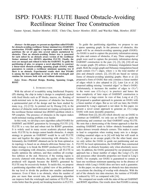
Fig. 1 depicts the outputs after various stages of the
algorithm.
A. Previous Approaches
III. OASG GENERATION
We first define what we meant by an obstacle-avoiding
spanning graph.
Definition 1 Given an edge e(u, v) and an obstacle b,
e is completely blocked by b if every monotonic Manhattan
path connecting u and v intersects with a boundary of b.
Definition 2 Given a set of m pins and k obstacles, an
undirected graph G = (V, E) connecting all pin and corner
vertices is called an OASG if none of its edges is completely
blocked by an obstacle.
Although Definition 2 does not necessitate a linear number
of edges for an OASG, in order to have a fast runtime
it is desired to limit the solution space. In the past, there
have been a couple of efforts to construct an OASG with a
linear number of edges. Shen et al. [2] suggested a quadrant
approach in which each point can connect in four quadrants
in the plane formed by horizontal and vertical line going
through the point. Shen did not clearly explain their algorithm
in the paper.
Long et al. [7] recently described an O(n log n)-time approach
for OASG generation with a linear number of edges
by considering quadrant partition of the plane. They suggested
scanning along ±45 ◦ lines and maintaining an active vertex
list, a set of vertices in the graph which are not yet connected
to their nearest neighbor. After scanning any vertex v, they
search for its nearest neighbor u in the active vertex list, such
that the edge (u, v) is not completely blocked by any obstacle
in the graph. This is followed by deletion of u from the list
and addition of v in the list.
We found that the OASG generation algorithm in [7] has a
few shortcomings. First in their algorithm, the nearest neighbor
for any vertex in a quadrant is contingent upon the direction
of scanning which means they have to scan along all four
quadrants of a vertex in order to capture its connectivity
information. Second, in the absence of obstacles, their algorithm
cannot guarantee the presence of at least one minimum
spanning tree in their spanning graph. Third, their algorithm
cannot handle abutting obstacles due to minor mistakes in the
inequality conditions.
0
0 1000 2000 3000 4000 5000 6000 7000 8000 9000 10000
(a) OASG
0
0 1000 2000 3000 4000 5000 6000 7000 8000 9000 10000
0
0 1000 2000 3000 4000 5000 6000 7000 8000 9000 10000
(b) MTST
0
0 1000 2000 3000 4000 5000 6000 7000 8000 9000 10000
B. Our Approach for OASG
In [18], Zhou et al. proposed an elegant algorithm to
generate a spanning graph with a linear number of edges
guaranteed to contain a minimum rectilinear spanning tree
on an obstacle-free plane by considering octant partition of
the plane. So, we also propose an OASG algorithm based
on octant partition. Fig. 2(a) and Fig. 2(b) describe octant
partition for a pin vertex and an obstacle corner, respectively.
Fig. 1.
RC01
(c) OPMST
(d) OARSMT
Demonstration of the major steps of FOARS using the benchmark
A property of octant partition is that a contour of equidistant
points from any point forms a line segment in each region.
In regions R 1 ,R 2 ,R 5 ,R 6 , these segments are captured by an
equation of the form x+y = c for some constant c; in regions

3
Fig. 2.
(a) Pin vertex
(b) Obstacle corner
Octant partition for a pin vertex and an obstacle corner
R 3 ,R 4 ,R 7 ,R 8 , they are described by the equation x − y = c
for some constant c. Now this property can be exploited when
we generate an obstacle-avoiding spanning graph.
The pseudocode for OASG generation for R 1 is provided in
Fig. 3. As R 1 and R 2 both follow the same sweep sequence we
process them together in one pass. It is worth noting that it is
sufficient to sweep for R 1 , R 2 , R 3 and R 4 only. For any point,
we only need to sweep twice to determine its connectivity
information once for R 1 /R 2 and once for R 3 /R 4 .
point we delete all the points in S(v) from A active (line 8)
and add v to A active (line 18).
In order to determine if an edge is blocked by an obstacle,
we maintain two active obstacle boundary lists, A bottom for
the bottom boundaries and A left for the left boundaries. It is
evident that if an edge is blocked by an obstacle in R 1 , it will
intersect with either its bottom or its left boundary. Next, if
our scanned vertex is the bottom left corner of an obstacle,
its bottom boundary is added to A bottom and its left boundary
is added to A left . It implies that both the left and the bottom
boundaries of that obstacle become active. When we come
across the top left (bottom right) corner, the corresponding
boundary is removed from A left (A bottom ) implying that the
left (bottom) boundary for that obstacle becomes inactive at
that point (lines 12 and 15).
To explain lines 13 to 17, let us refer to Fig. 4 where vertex
b is the bottom right corner of an obstacle. It is easy to see
that if any vertex u lying within the 45 − 45 − 90 triangle
shown is still in A active after scanning b, it can be removed
from A active . Since in this case all vertices in R 1 of u are
completely blocked from u by the obstacle.
Algorithm: OASG Generation for R 1
Fig. 3.
1 A active = A bottom = A left = ∅
2 for all v ∈ V in increasing (x + y) order do
3 S(v) = ∅
4 for all u ∈ A active which have v in their R 1 do
5 Add u to S(v)
6 end for
7 Connect v to the nearest point u ∗ ∈ S(v) such that
e(u ∗ , v) is not completely blocked
by obstacle boundaries in A bottom and A left
8 Delete all points in S(v) from A active
9 if v is a bottom left corner then
10 Add the bottom boundary containing v to A bottom
and the left boundary containing v to A left
11 else if v is a top left corner then
12 Delete the left boundary containing v from A left
13 else if v is a bottom right corner then
14 Determine the bottom boundary B containing v
15 Delete B from A bottom
16 Delete from A active all points which are
completely blocked by B
17 end if
18 Add v to A active
19 end for
Pseudocode for OASG generation algorithm
For octants R 1 and R 2 , we sweep on a list of vertices in
V which contains both pins as well as obstacle corners with
respect to increasing (x+y). During sweeping we maintain an
active vertex list A active . An active vertex is a vertex whose
nearest neighbor in R 1 still needs to be discovered.
For the currently scanned vertex v, while looking in R 5
of v we extract a subset S(v) from A active . Any node u in
this subset S(v) has v in R 1 (lines 3 to 6). We connect v
to its nearest neighbor u ∗ in S(v) for which, e(u ∗ , v) is not
completely blocked (line 7). After connecting with the nearest
Fig. 4. Any vertex within the lightly shaded triangle is completely blocked
by boundary (a,b).
We have the following lemma that relates our obstacleavoiding
spanning graph generation algorithm to the
obstacle-free spanning graph generation algorithm in [18].
Lemma 1 The algorithm of Zhou et al. [18] is a special case
of our OASG generation algorithm
Proof: If we consider an instance which has no obstacle, then
we can simply ignore the blockage check in line 7 and lines
9 to 17 from the algorithm in Fig. 3. The resulting algorithm
would be exactly the same as the spanning graph generation
algorithm in [18].
□
Corollary 1 In the absence of obstacle, our OASG generation
algorithm generates a spanning graph that contains at least
one minimum rectilinear spanning tree of the given pins.
Proof: By Lemma 1, our OASG algorithm generates
the same result as the obstacle-free spanning graph generation
algorithm in [18] when there is no obstacle. Moreover, it has
been proved in [18] that the obstacle-free spanning graph
generated is guaranteed to contain at least one minimum

4
spanning tree of the given pins.
C. An Efficient Implementation
In this section we show how to efficiently perform the
following fundamental operations in the OASG generation
algorithm: 1) Given a vertex v, find the subset of points in
A active which have v in their R 1 ; 2) given an edge, check if
it is completely blocked by any obstacle boundary in A bottom
or A left ; and 3) given a bottom boundary of an obstacle,
find all points in A active which are completely blocked by the
boundary. We address these issues one by one in the following
paragraphs.
To find the subset of points in A active that have a given
point in their R 1 , we first state and prove two lemmas and a
corollary for our OASG generation algorithm. Similar ideas
have been outlined in [18].
Lemma 2 Point v is in the R 1 region of point p if
and only if x p ≤ x v and x p − y p ≥ x v − y v .
Proof: By definition, the R 1 region of p is the region
to the right of the vertical line passing through p and above
the line with slope = 1 passing through p (see Fig. 2). In other
words, point v is in the R 1 region of p if and only if x p ≤ x v
and yv−yp
x v−x p
≥ 1. Rearranging the terms, the necessary and
sufficient condition is x p ≤ x v and x p − y p ≥ x v − y v . □
Lemma 3 At any time, no point in the active set can
be in the R 1 region of another point in the set.
Proof: Before we add a new point v to the active set
(line 18), we would delete all points in the active set that
have v in their R 1 regions (line 8). In addition, any point
already in the active set cannot be in the R 1 region of point
v as we are processing in increasing (x + y) order. Hence,
no point in the active set can be in the R 1 region of another
point in the set at any time.
□
Corollary 2 For any two points p and q in the active
set, we have x p ≠ x q , and if x p < x q then x p −y p ≤ x q −y q .
Proof: Assume points p and q are in the active set.
Then we cannot have x p = x q , otherwise p would be
in the R 1 region of q or vice versa by Lemma 2 which
contradicts Lemma 3. And we cannot have x p < x q and
x p − y p ≥ x q − y q , otherwise q would be in the R 1 region of
p by Lemma 2 which again contradicts Lemma 3. Hence, the
corollary is proved.
□
To facilitate finding the points in A active that have a
given point in their R 1 regions, we keep the points in A active
in increasing order of their x-coordinate. To find the subset
of points which have v in their R 1 , we first find the largest
x in A active such that x ≤ x v . We then scan A active in
decreasing order of x until x − y < x v − y v . Note that by
Corollary 2, decreasing order of x automatically implies
non-increasing order of x − y. Any point in between has
□
x ≤ x v and x − y ≥ x v − y v , and hence has v in its R 1 by
Lemma 2. We use a balanced binary search tree to implement
A active in order to have O(log n) query operation to find the
largest x in A active such that x ≤ x v .
An edge e(u, v) formed by points (x u , y u ) and (x v , y v )
is completely blocked by a bottom obstacle boundary (a, b)
formed by the points (x a , y h ) and (x b , y h ), if and only if,
y u < y h < y v , x a < x u , and x b > x v . Note that at line 7,
all bottom boundaries satisfying the condition must be present
in the list A bottom . We use a balanced binary search tree data
structure for A bottom with the y-coordinate of a boundary as
a key value. If there are k bottom boundaries between y u and
y v , it takes takes O(log n + k) time to check if any of them
blocks edge e. Checking if an edge is completely blocked by
a left boundary can be done similarly.
To determine all the completely blocked vertices u in
A active by a horizontal boundary (a, b) in line 16, we need to
check if y u < y h , x a < x u and x u −y u +y h ≤ x b (the lightly
shaded region in Fig. 4). Since we already have A active as a
sorted list in increasing x we can check all points which lie
between x a and x b and test for the above conditions to see if
they are completely blocked.
In [16] we made a claim about runtime complexity of
the overall algorithm being O(n log n). It has been recently
brought to our attention that there may exists extreme cases
for which the total time spent by line 7 over all iterations is
O(n 2 ). We concede with the argument but our algorithm is
extremely fast for all practical purposes as indicated by our
experimental results and it results in an OASG with a linear
number of edges which limits the solution space resulting in
better runtime complexity for subsequent stages.
A. MTST Generation
IV. OPMST GENERATION
After capturing the initial connectivity among pin vertices,
the next logical step is to extract a minimum terminal spanning
tree (MTST) from the OASG that connects all pin vertices
and avoid obstacles. Shen et al. [2] and Lin et al. [6] both
use an indirect approach for this step. They first construct a
complete graph over all pin vertices where the edge weight is
the shortest path length between the two pin vertices. On this
complete graph they use either Prim’s or Kruskal’s algorithm
to obtain a MST. Although it is effective, the approach
described above seems to be an overkill as it is unnecessary
to construct a complete graph when we already have OASG.
Back in the 80’s, Wu et al. [17] suggested a method using
Dijkstra’s and Kruskal’s algorithms on a graph similar to an
OASG to obtain a MTST. Recently, Long et al. [8] adopted
their approach to solve the problem on the OASG.
In this paper, we adopt the approach based on the extended
Dijkstra’s algorithm and the extended Kruskal’s algorithm as
defined in [8]. For every corner vertex in the OASG, we want
to connect it with the nearest pin vertex. This can be easily
done using Dijkstra’s shortest path algorithm considering
every pin vertex as a source. After running the extended
Dijkstra’s algorithm we are left with a forest of m terminal
trees, m being the number of pin vertices. The root of every

5
terminal tree in the forest obtained above is a pin vertex.
In order to connect all disjoint trees we use the extended
Kruskal’s algorithm on the forest. A priority queue Q is used
to store the weights of all possible edges termed as bridge
edges in [8] which can be used for linking the trees.
Definition 4 [8] An edge e(u, v) is called a bridge
edge if its two end vertices belong to different terminal trees.
From Definition 4, it can be deduced that if each tree
was a single vertex in the graph then bridge edges will be
the edges connecting these vertices and we can use Kruskal’s
algorithm to obtain a MST in such a graph. The extended
Kruskal’s algorithm is simply an extended version of the
original Kruskal’s algorithm tailored to obtain a MST in a
forest. It is important to note that in case we do not have any
obstacle, the extended Dijkstra’s algorithm will not make any
change in the graph and the extended Kruskal will simply
work on a spanning graph.
B. OPMST Construction
We note that a sparse OASG does not always have direct
connections between the pin vertices even if one is allowed.
This is due to a neighboring corner vertex being nearer than
the other pin vertex in the same region. These indirect detour
paths are unnecessary and if not taken care of can lead to a
significant loss of quality. We note that the algorithm proposed
by [8] failed to address this issue. On the other hand, we
address this problem by constructing an obstacle penalized
minimal spanning tree (OPMST) from the MTST by removing
all the corner vertices and storing detour information as the
weight of an edge.
To construct an OPMST, we follow a simple strategy. For
any corner vertex v, we find the nearest neighboring pin vertex
u. We connect all the pin vertices originally connected with
v to u and delete v. We update their weights as their original
weight plus the weight of e(u, v). This method guarantees
that in case we have a major detour between two pin vertices
due to an obstacle, the weight of that edge will corroborate
this fact. In other words we can say that the edge would be
penalized for the obstacles in its path.
V. OAST GENERATION
This step differentiates our algorithm from [2], [6]–[8]. We
exploit the extremely fast and efficient Steiner tree generation
capability of FLUTE [15] for low degree nets. In order to
embed FLUTE in our problem, we designed an obstacle
aware version of FLUTE, OA-FLUTE. As OA-FLUTE is less
effective for high degree nets and dense obstacle region, we
partition a high degree net into subnets guided by the OPMST
obtained from the previous step. The subproblems obtained
after partitioning are passed on to OA-FLUTE for obstacle
aware topology generation. It is termed as obstacle-aware
because the nodes of the tree are placed in their appropriate
locations considering obstacles around them.
Fig. 5 and Fig. 8 describe the pseudocodes for the Partition
and OA-FLUTE functions. It is evident that both functions are
recursive functions. Let us first explain the Partition function.
A. Partition
Function: Partition(T )
Input: An OPMST T
Output: An OAST
1 if (∃ a completely blocked edge e) then
2 /∗ Refer to Fig. 6 ∗/
3 e(u, v) is to be routed around obstacle edge e(a, b)
4 Let T = T 1 + e(u, v) + T 2
5 T 1 = T 1 + e(u, a)
6 T 2 = T 2 + e(u, b)
7 T ′ = Partition(T 1) ∪ Partition(T 2)
8 else if (|T | > HIGH THRESHOLD) then
10 /∗ Refer to Fig. 7(a) ∗/
11 Let e(u, v) be the longest edge s.t.
T = T 1 + e(u, v) + T 2 with |T 1| ≥ 2 and |T 2| ≥ 2
12 T ′ = Partition(T 1) ∪ Partition(T 2)
13 /∗ Refer to Fig. 7(b) ∗/
14 Refine T ′ using OA-FLUTE(N”)
15 where N” is a set of pin vertices around e(u, v) in T ′
16 else
17 T ′ = OA-FLUTE(N)
18 where N is set of all vertices in T
19 end if
20 return T ′
Fig. 5.
Pseudocode for the Partition function
The input to the Partition function is an OPMST obtained
from the last step and the output is an obstacle-aware Steiner
tree (OAST). An OAST is a Steiner tree in which the Steiner
nodes have been placed considering the obstacles present in
the routing region to minimize the overall wirelength. The
following two criteria are set for partitioning pin vertices. The
first criterion is to determine if any edge is completely blocked
by an obstacle. The second criterion is to check if the size of
OPMST is more than the HIGH THRESHOLD defined.
Fig. 6.
Fig. 7.
An example illustrating first criterion for partitioning
(a) Partitioning
(b) Local refinement
An example illustrating second criterion for partitioning
As can be clearly seen in Fig. 6 that for an overlap free
solution, we have to route around the obstacle. Therefore, it

6
seems logical to break the tree at edge (u, v). We know that
OA-FLUTE can efficiently construct a tree when the number
of nodes is less than the HIGH THRESHOLD value. If the
size of the tree is still more than the HIGH THRESHOLD
after breaking at the blocking obstacles, we need to break the
tree further. In this case, we look for the edge with the largest
weight on the tree and delete that edge, refer to Fig. 7(a).
Based on the above mentioned criteria, if we break an
obstacle edge, we simply include corner vertices in the tree
and divide the two trees as shown in Fig. 6. Else, if we break
at the edge with largest weight, we delete that edge and make
sure that it does not contain any leaf of the tree as shown in
Fig. 7(a).
After breaking an edge, we make recursive calls to the
Partition function using two subtrees. When the size of the
tree becomes less than the HIGH THRESHOLD, we pass the
nodes of the tree to OA-FLUTE function. The OA-FLUTE
function returns an OAST. After returning from OA-FLUTE in
Partition, if the partition was performed on an obstacle edge,
we simply merge two Steiner trees using the same obstacle
edge. In case the partition was performed on the longest edge,
we explore an opportunity to further optimize wirelength. We
merge the two trees on the longest edge and then search
the region around the longest edge to extract neighboring
pin vertices, refer to lines 12-15 in Fig. 5 and Fig. 7(b).
This refinement is same as the local refinement proposed in
[15]. We pass this set of nodes to OA-FLUTE for further
optimization.
constructs a Steiner tree without considering obstacles. This
tree can have two kinds of overlap 1) an edge completely
blocked by an obstacle, 2) a Steiner node falling on any
obstacle. We handle both of these cases differently.
To handle the first case, refer to Fig. 9, we break the Steiner
tree into two subtrees including corner points of the obstacle
as in Fig. 9(b) and make recursive calls to OA-FLUTE. We
selectively prune the number of recursive calls based on the
size of the tree in order to strike a balance between run-time
and quality.
(a) Completely blocked Edge
(c) Merging excluding corners
Fig. 9.
(b) Subtrees before merging
OA-FLUTE: Handling an edge completely blocked by an obstacle
B. OA-FLUTE
Function: OA-FLUTE(N)
Input: A set of nodes N
Output: An OAST
1 T ′ = FLUTE(N)
2 if (∃ a completely blocked edge e) then
3 e(u, v) is to be routed around obstacle boundary e(a, b)
4 /∗ Refer to Fig. 9 ∗/
5 Let N = N 1 ∪ N 2
6 N 1 = N 1 ∪ {a}
7 N 2 = N 2 ∪ {b}
8 T ′ = OA-FLUTE(N 1) ∪ OA-FLUTE(N 2)
9 else if (∃ Steiner Node S that falls on any obstacle) then
10 /∗ Refer to Fig. 10 ∗/
11 Let a 1, a 2, ... , a D be the intersection points with the
obstacle ordered in anti-clockwise direction
12 Let N = N 1 ∪ N 2 ∪ ... ∪ N D ∪ {S}
13 Let (a u, a v) be the segment with largest weight
14 for (i = a v to a u in anti-clockwise order) do
15 N i = N i∪ corner vertices along the path next to N i
16 end for
17 T ′ = OA-FLUTE(N 1) ∪ ..... ∪ OA-FLUTE(N D)
18 end if
19 return T ′
Fig. 8.
Pseudocode for the OA-FLUTE function
The purpose of OA-FLUTE function is to form an OAST.
It begins by calling FLUTE on the set of input nodes. FLUTE
(a) Removing longest
segment
Fig. 10.
(b) Subtrees before
merging
(c) Merging excluding
corners
OA-FLUTE: Handling Steiner node falling on an obstacle
To handle the second case, we devised a special technique.
We pick an obstacle which has a Steiner node on top of it. For
every boundary of this obstacle intersecting with the Steiner
tree, we extract a set of nodes N i which includes the pin
vertices in the tree near to that boundary. In Fig. 10(a) we
have a single Steiner node inside the obstacle intersecting at
a 1 , a 2 and a 3 , with the right, top and left boundary of the
obstacle, respectively. We extract three set of pin vertices N 1 ,
N 2 and N 3 from the original Steiner tree for the right, top and
left boundary, respectively. The points a 1 , a 2 and a 3 divide the
obstacle outline into three segments as shown in Fig. 10(a).
We then find the longest segment (the light shaded segment
(a 3 , a 1 ) in Fig. 10(a)). We then traverse from one endpoint of
the longest segment to the other endpoint via other segments
in an anti-clockwise direction, for example, from a 1 to c 1 to
a 2 to c 2 to a 3 in Fig. 10(a). While moving along the other
segments, we keep adding corner vertices to the corresponding
N i ’s e.g. c 1 gets added to both N 1 and N 2 and c 2 gets added

7
to both N 2 and N 3 in Fig. 10(b). We then recursively call
OA-FLUTE for all N i ’s thus formed.
As our goal with OA-FLUTE is to determine befitting
locations for Steiner nodes we exclude all corner vertices
when we finally merge the subtrees. Fig. 9(c) and Fig. 10(c),
show the final Steiner trees after excluding corners while
merging. The reason for not adding corner vertices in this
step is twofold. First, it is not desirable to further restrict
the solution when we already did once in Partition function.
Second, we want our OA-FLUTE to be a generic function
which can preserve the number of pin-vertices provided to it,
adding corner vertices would increase them.
C. Fast Implementation with Obstacle Tree Data Structure
To create an OAST, OA-FLUTE performs two major tasks.
It tries to remove all completely blocked edges and removes
all Steiner nodes falling on any obstacle. In order to perform
these tasks, it requires to check each edge and Steiner node
of the tree against all obstacles if we use a naive list data
structure to represent the obstacles. Our experiments in [16]
were performed based upon this simple approach.
In this paper, we propose an efficient obstacle tree (OBTree)
data structure. An OBTree is a balanced binary tree in which
we bin obstacles in their enclosing regions. We start with
a region which encloses all obstacles. After that, depending
upon the dimensions of the region, we slice the region either
vertically or horizontally into two parts. After dividing the
region into two halves we create two similar problems as
before. We use recursion to further split these regions until
there is only one obstacle inside each bin.
Fig.11 describes the pseudocode used by FOARS to create
an obstacle tree. The procedure CreateOBTree is provided with
a list of obstacles. In case the region enclosing the obstacles
has larger width than height, we divide the obstacles into
two parts based upon the x-coordinates of their bottom left
corners. Otherwise, the y-coordinates of bottom left corners
of obstacles are used.
OBTree is extremely efficient for searching if an edge is
completely blocked by any obstacle or if a Steiner node falls
on any obstacle. The pseudocode in Fig. 12 and Fig. 13 are
recursive procedures to perform above mentioned tasks.
VI. OARSMT GENERATION
The OAST obtained from last step does not guarantee that
rectilinear path for a pin-to-pin connection is obstacle free. In
this step, we rectilinearize every pin-to-pin connection avoiding
obstacles to generate an OARSMT. For every Manhattan
connection between two pins we can have two L-shape paths.
On the basis of the obstacles inside the bounding box formed
by an edge, we can divide all the possible scenarios into
four categories: 1) both L-paths are clean 2) both L-paths are
blocked by the same obstacle 3) only one L-path is blocked
4) both L-paths are blocked but not by the same obstacle. We
discuss these scenarios one by one in the following paragraphs.
For the first case, even though we can rectilinearize using
any L-path, we instead create a slant edge at this stage to
leave the scope for improvement in V-shape refinement. For
Function: CreateOBTree(OB, K)
Input: A set of obstacles OB = {O 1, O 2, . . . , O K}
Number of obstacles K
Output: An obstacle tree OBTree
1 OBTree → OB = OB
2 OBTree → x MIN = Leftmost boundary of OB
3 OBTree → x MAX = Rightmost boundary of OB
4 OBTree → y MIN = Bottommost boundary of OB
5 OBTree → y MAX = Topmost boundary of OB
6 OBTree → C 1 = NULL
7 OBTree → C 2 = NULL
8 if (K > 1) then
9 H = ⌈K/2⌉
10 if (OBTree → x MAX − OBTree → x MIN
> OBTree → y MAX − OBTree → y MIN ) then
11 OB L = {first H obstacles in increasing order of x}
12 OB R = OB − OB L
13 OBTree → C 1 = CreateOBTree(OB L, H)
14 OBTree → C 2 = CreateOBTree(OB R, K − H)
15 else
16 OB B = {first H obstacles in increasing order of y}
17 OB T = OB − OB B
18 OBTree → C 1 = CreateOBTree(OB B, H)
19 OBTree → C 2 = CreateOBTree(OB T , K − H)
20 end if
21 end if
22 return OBTree
Fig. 11.
Fig. 12.
Pseudocode for creating an OBTree
Function: CheckSteinerNode(α, π)
Input: Steiner node α; obstacle tree node π
Output: Set of obstacles under π on which α falls
1 Let R =region enclosed by π
2 if (α does not lie inside R) then
3 return ∅
4 else if (π contains a single obstacle O) then
5 return {O}
6 else
7 Let π 1 and π 2 be children of π
8 OB 1 = CheckSteinerNode(α, π 1)
9 OB 2 = CheckSteinerNode(α, π 2)
10 OB = OB 1 ∪ OB 2
11 return OB
12 end if
Pseudocode for checking if a Steiner node falls on any obstacle
the second case, we have no option but to go outside the
bounding box and pick the least possible detour.
For the third case, we route inside the bounding box, since
there exists a path. We break the edge into two sub problems
on the corner of an obstacle along the blocked L-path. We
recursively solve these sub problems to determine an obstacleavoiding
path. If the wirelength of this path is same as the
Manhattan distance between the pins, we accept the solution,
else we route along the unblocked L-path. It is noteworthy that
for this case we could have directly accepted the unblocked
L-path. In order to create more slant edges, and hence, further
scope for V-shape refinement, we searched for a route along
the blocked L-path avoiding obstacles. For the last case where

8
Function: CheckEdge(e, π)
Input: Edge e; obstacle tree node π
Output: Set of obstacles under π completely blocking e
1 Let R =region enclosed by π
2 if (e cannot completely blocked by any rectangle in R) then
/* i.e., e can completely avoid π without detour */
3 return ∅
4 else if (π contains a single obstacle O) then
5 return {O}
6 else
7 Let π 1 and π 2 be children of π
8 OB 1 = CheckEdge(e, π 1)
9 OB 2 = CheckEdge(e, π 2)
10 OB = OB 1 ∪ OB 2
11 return OB
12 end if
Fig. 13.
Pseudocode for checking if an edge is completely blocked
both L-paths are blocked but not by the same obstacle, we
determine obstacle-avoiding routes using the same recursive
approach as mentioned above for both L-paths and pick the
shortest one.
VII. REFINEMENT
We perform a final V-shape refinement to improve total
wirelength. This refinement includes movement of Steiner
node in order to discard extra segments produced due to
previous steps. The concept of refinement is similar to the
one that determines a Steiner node for any three terminals. The
coordinates of the Steiner node are the median value of the
x-coordinates and median value of the y-coordinates. Fig. 14
illustrates a potential case for V-shape refinement and output
after refinement. This refinement comes handy in improving
the overall wirelength by 1% to 2%.
Fig. 14.
V-shape refinement case and refined output
VIII. EXPERIMENTAL RESULTS
We implemented our algorithm in C. The experiments
were performed on a 3GHz AMD Athlon 64 X2 Dual Core
machine. We requested for binaries from Long et al. [8],
Lin et al. [6], Liang et al. [10] Liu et al. [11] [12] and
ran them on our platform. Five industrial testcases (IND1 -
IND05), twelve circuits from [6] (RC01-RC12), five randomly
generated benchmark circuits (RT01-RT05) [6] and five large
benchmark circuits (RL01-RL05) generated by [8].
A. OARSMT Experimental Results
Table I and II shows wirelength and runtime comparison on
benchmarks containing obstacles. We determined experimentally
that HIGH THRESHOLD value of 20 works the best.
Wirelength
Runtime (s)
Benchmark m k FOARS [16] FOARS FOARS [16] FOARS
RC01 10 10 25980 25980 0.00 0.00
RC02 30 10 42110 42110 0.00 0.00
RC03 50 10 56030 56030 0.00 0.00
RC04 70 10 59720 59720 0.00 0.00
RC05 100 10 75000 75000 0.00 0.00
RC06 100 500 81229 81229 0.03 0.03
RC07 200 500 110764 110764 0.03 0.03
RC08 200 800 116047 116047 0.06 0.05
RC09 200 1000 115593 115593 0.08 0.06
RC10 500 100 168280 168280 0.02 0.02
RC11 1000 100 234416 234416 0.04 0.03
RC12 1000 10000 756998 756998 2.04 1.19
RT01 10 500 2191 2191 0.01 0.00
RT02 50 500 48156 48156 0.02 0.02
RT03 100 500 8282 8282 0.03 0.03
RT04 100 1000 10330 10330 0.07 0.06
RT05 200 2000 54598 54634 0.21 0.15
IND1 10 32 604 604 0.00 0.00
IND2 10 43 9500 9500 0.00 0.00
IND3 10 59 600 600 0.00 0.00
IND4 25 79 1129 1129 0.00 0.00
IND5 33 71 1364 1364 0.00 0.00
RL01 5000 5000 483027 483027 3.13 1.15
RL02 10000 500 637753 637753 1.36 1.18
RL03 10000 100 640902 640902 1.15 1.13
RL04 10000 10 697125 697125 1.55 1.57
RL05 10000 0 728438 728670 1.66 0.12
(0.999) (1) 11.54(1.59) 7.23(1)
TABLE I
WIRELENGTH AND RUNTIME COMPARISON BETWEEN FOARS [16] AND
CURRENT RESULTS
Table I shows our newest results as compared with results
published in [16]. Using OBTree in FOARS we were able
to cut down the runtime by 59% with negligible increase in
wirelength. The reason for the slight increase in wirelength is
that we decided to disable the refinement step for instances
with no obstacle (RL05 in Table I). Based on experiments,
we determine that if we remove the refinement step for
instances with no obstacles, we gain significantly in runtime
with negligible loss in quality (see Table III).
Columns 4 and 5 of Table II show that FOARS outperforms
Lin et al. [6] by 2.3% and Long et al. [8] by 2.7%. Columns
6, 7 and 8 indicate that FOARS has similar wirelength results
as compared with Liang et al. [10] and Liu et al. [11] [12].
For the runtime in Table II, we are now 84% faster than Long
et al. [8] on average. We are 46 times faster than [10] and 123
times faster than [6].Our runtime is slower as compared with
Liu et al. [11] [12].
B. RSMT Experimental Results
As mentioned before, RSMT can be seen as a special case
for OARSMT. In an effort to construct a single solution for
OARSMT and RSMT generation, we performed experiments
on our existing benchmarks after deleting obstacles. As shown
in Table III, we compare our results with Long et al. [8] and
Liang et al. [10]. We could not compare our results with [11]
and [12] as their binaries could not run on cases with no
obstacles. We also compared our results with FLUTE-2.5 [15]
which is the same version of FLUTE as used inside FOARS.
Our result for wirelength is the best among all the algorithms
and is 2.6% better as compared with FLUTE-2.5.
Compared with FLUTE-2.5, which has been demonstrated to

9
Wirelength
Runtime (s)
Benchmark m k Lin [6] Long [8] Liang [10] Liu [11] Liu [12] FOARS Lin [6] Long [8] Liang [10] Liu [11] Liu [12] FOARS
RC01 10 10 27790 26120 25980 26740 26040 25980 0.00 0.00 0.01 0.00 0.00 0.00
RC02 30 10 42240 41630 42010 42070 41570 42110 0.00 0.00 0.02 0.00 0.00 0.00
RC03 50 10 56140 55010 54390 54550 54620 56030 0.00 0.00 0.00 0.00 0.00 0.00
RC04 70 10 60800 59250 59740 59390 59860 59720 0.00 0.00 0.01 0.00 0.00 0.00
RC05 100 10 76760 76240 74650 75440 74770 75000 0.00 0.00 0.01 0.00 0.00 0.00
RC06 100 500 84193 85976 81607 81903 81854 81229 0.10 0.08 0.50 0.01 0.02 0.03
RC07 200 500 114173 116450 111542 111752 110851 110764 0.18 0.09 0.60 0.01 0.03 0.03
RC08 200 800 120492 122390 115931 118349 116132 116047 0.31 0.15 1.16 0.02 0.04 0.05
RC09 200 1000 117647 118700 113460 114928 113559 115593 0.40 0.22 1.53 0.02 0.05 0.06
RC10 500 100 171519 168500 167620 167540 167460 168280 0.20 0.03 0.18 0.00 0.01 0.02
RC11 1000 100 237794 234650 235283 234097 236018 234416 0.74 0.06 0.83 0.01 0.02 0.03
RC12 1000 10000 803483 832780 761606 780528 762435 756998 55.09 3.80 186.3 0.36 1.20 1.19
RT01 10 500 2289 2379 2231 2259 2193 2191 0.03 0.06 0.19 0.01 0.01 0.00
RT02 50 500 48858 51274 47297 48684 47488 48156 0.05 0.06 0.55 0.01 0.02 0.02
RT03 100 500 8508 8554 8187 8347 8231 8282 0.10 0.06 0.21 0.01 0.02 0.03
RT04 100 1000 10459 10534 9914 10221 9893 10330 0.22 0.23 0.37 0.02 0.04 0.06
RT05 200 2000 54683 55387 52473 53745 52509 54634 0.96 0.66 3.18 0.04 0.12 0.15
IND1 10 32 632 639 619 626 604 604 0.00 0.00 0.00 0.00 0.00 0.00
IND2 10 43 9700 10000 9500 9700 9600 9500 0.00 0.00 0.00 0.00 0.00 0.00
IND3 10 59 632 623 600 600 600 600 0.00 0.00 0.00 0.00 0.00 0.00
IND4 25 79 1121 1130 1096 1095 1092 1129 0.00 0.00 0.00 0.00 0.00 0.00
IND5 33 71 1392 1379 1360 1364 1374 1364 0.00 0.00 0.00 0.00 0.00 0.00
RL01 5000 5000 492865 491855 481813 483134 483199 483027 106.66 3.58 27.14 0.27 0.63 1.15
RL02 10000 500 648508 638487 638439 636097 640435 637753 159.09 1.27 29.45 0.23 0.37 1.18
RL03 10000 100 652241 641769 642380 640266 644276 640902 153.95 1.08 23.35 0.22 0.32 1.13
RL04 10000 10 709904 697595 699502 696111 700937 697125 195.25 0.97 22.00 0.24 0.29 1.57
RL05 10000 0 741697 728585 730857 - - 728670 217.88 0.96 33.64 - - 0.12
891.25 13.36 331.235 1.48 3.19 7.23
Norm 1.024 1.027 0.995 1.004 0.994 1 123.26 1.84 45.81 0.20 0.44 1
TABLE II
WIRELENGTH AND RUNTIME COMPARISON. m IS THE NUMBER OF PIN VERTICES AND k IS THE NUMBER OF OBSTACLES. THE VALUES IN THE LAST ROW
ARE NORMALIZED OVER OUR RESULTS FOR BOTH WIRELENGTH AS WELL AS RUNTIME
Wirelength
Runtime (s)
Benchmark m k Long [8] Liang [10] FLUTE-2.5 [15] Ours Long [8] Liang [10] FLUTE-2.5 [15] FOARS
RC01 10 0 25290 25290 25290 25290 0.00 0.00 0.00 0.00
RC02 30 0 40100 40630 39920 39920 0.00 0.00 0.00 0.00
RC03 50 0 52560 52440 53400 53050 0.00 0.00 0.00 0.00
RC04 70 0 55850 55720 57020 55380 0.00 0.00 0.00 0.00
RC05 100 0 72820 71820 73370 72170 0.00 0.00 0.00 0.00
RC06 100 0 77886 78068 80057 77633 0.00 0.00 0.00 0.00
RC07 200 0 106591 107236 109232 106581 0.01 0.07 0.00 0.00
RC08 200 0 109625 109059 112787 108928 0.00 0.03 0.00 0.00
RC09 200 0 109105 108101 112460 108106 0.01 0.02 0.00 0.00
RC10 500 0 164940 164450 170270 164130 0.02 0.17 0.00 0.00
RC11 1000 0 233743 235284 245325 233647 0.06 0.70 0.00 0.00
RC12 1000 0 755332 764956 798742 755354 0.04 0.75 0.00 0.00
RT01 10 0 1817 1817 1817 1817 0.01 0.00 0.00 0.00
RT02 50 0 44930 46109 45291 44416 0.00 0.00 0.00 0.00
RT03 100 0 7677 7777 7811 7749 0.00 0.00 0.00 0.00
RT04 100 0 7792 7826 7826 7792 0.00 0.00 0.00 0.00
RT05 200 0 43335 43586 44809 43026 0.00 0.00 0.00 0.00
IND1 10 0 614 619 604 604 0.00 0.00 0.00 0.00
IND2 10 0 9100 9100 9100 9100 0.00 0.00 0.00 0.00
IND3 10 0 590 590 587 587 0.00 0.00 0.00 0.00
IND4 25 0 1092 1092 1102 1102 0.00 0.00 0.00 0.00
IND5 33 0 1314 1304 1307 1307 0.00 0.00 0.00 0.00
RL01 5000 0 472392 473905 501480 472818 0.30 11.39 0.05 0.05
RL02 10000 0 637131 641722 674042 636895 0.95 32.45 0.25 0.12
RL03 10000 0 641289 650343 674950 640580 0.95 33.04 0.26 0.12
RL04 10000 0 697712 699617 740270 697239 0.99 32.26 0.25 0.13
RL05 10000 0 728595 730857 778313 728670 1.05 34.52 0.26 0.12
(1.002) (1.005) (1.026) (1) 4.52(7.75) 145.37(249) 1.104(1.89) 0.58(1)
TABLE III
WIRELENGTH AND RUNTIME COMPARISON FOR BENCHMARK WITH NO OBSTACLES, I.E. k = 0 FOR ALL CASES

10
be significantly faster than other RSMT heuristics, FOARS
are 89% faster. FOARS are 7.75 and 249 times faster than [8]
and [10] respectively. Again FOARS performs much better
when we have large number of pin vertices in the benchmark
(RC12, RL01-RL05). The improvement in wirelength over
FLUTE-2.5 is due to the effective partitioning algorithm for
high-degree nets and the application of the local refinement
technique as shown in Fig. 7(b).
IX. CONCLUSION
In this paper, we have presented FOARS, an efficient
algorithm to construct OARSMT and RSMT based on extremely
fast and high-quality Steiner tree generation tool called
FLUTE. We proposed a novel OASG algorithm with linear
number of edges. We also proposed an obstacle aware version
of FLUTE, which generates OAST. Our top-down partition
approach empowers OA-FLUTE to handle high-degree nets
and dense obstacle region. Our implementation of OBTree
is simple and extremely efficient for checking blockage with
obstacles. Our results indicate that our approach is the best
tradeoff for quality and runtime for both OARSMT and RSMT
construction. Our experiments prove that FOARS obtains good
quality solution with excellent runtime as compared with its
peers.
ACKNOWLEDGEMENT
We acknowledge Lin et al. [6], Liang et al. [10], Long et
al. [8] and Liu et al. [11] [12] for sending us their binaries
for comparison and clearing our doubts, if any, with respect
to the results.
REFERENCES
[1] Yu Hu, Zhe Feng, Tong Jing, Xianlong Hong, Yang yang Ge, Xiaodong
Hu, and Guiying Yan. FORst: A 3-step heuristic for obstacle-avoiding
rectilinear Steiner minimal tree construction. In Proc. of JICS, pages
107–116, 2004.
[2] Zion Shen, Chris C. N. Chu, and Ying-Meng Li. Efficient rectilinear
Steiner tree construction with rectilinear blockages. In Proc. of ICCD,
pages 38–44, 2005.
[3] Yu Hu, Tong Jing, Xianlong Hong, Zhe Feng, Xiaodong Hu, and Guiying
Yan. An-OARSMan: Obstacle-avoiding routing tree construction with
good length performance. In Proc. of ASP-DAC, pages 630–635, 2006.
[4] Yiyu Shi, Paul Mesa, Hao Yao, and Lei He. Circuit simulation based
obstacle-aware Steiner routing. In Proc. of DAC, pages 385–388, 2006.
[5] Pei-Ci Wu, Jhih-Rong Gao, and Ting-Chi Wang. A fast and stable algorithm
for obstacle-avoiding rectilinear Steiner minimal tree construction.
In Proc. of ASP-DAC, pages 262–267, 2007.
[6] Chung-Wei Lin, Szu-Yu Chen, Chi-Feng Li, Yao-Wen Chang, and Chia-
Lin Yang. Obstacle-avoiding rectilinear Steiner tree construction based
on spanning graphs. In Proc.of IEEE Transactions on CAD of Integrated
Circuits and Systems, 27(4):643–653, 2008.
[7] Jieyi Long, Hai Zhou, and Seda Ogrenci Memik. An O(n log n) edgebased
algorithm for obstacle-avoiding rectilinear Steiner tree construction.
In Proc. of ISPD, pages 126–133, 2008.
[8] Jieyi Long, Hai Zhou, and Seda Ogrenci Memik. EBOARST: An efficient
edge-based obstacle avoiding-rectilinear Steiner tree construction
algorithm. In Proc. of IEEE Transactions on CAD of Integrated Circuits
and Systems, 27(12), 2008.
[9] Iris Hui-Ru Jiang, Shung-Wei Lin, and Yen-Ting Yu. Unification of
obstacle-avoiding rectilinear Steiner tree construction. In Proc. of SoCC,
pages 127–130, 2008.
[10] Liang Li and Evangeline F. Y. Young. Obstacle-avoiding rectilinear
Steiner tree construction. In Proc. of ICCAD, pages 523–528, 2008.
[11] Chih-Hung Liu, Shih-Yi Yuan, Sy-Yen Kuo, and Yao-Hsin Chou. An
O(n log n) path-based obstacle-avoiding algorithm for rectilinear Steiner
tree construction. In Proc. of DAC, pages 314–319, 2009.
[12] Chih-Hung Liu, Shih-Yi Yuan, Sy-Yen Kuo, and Jung-Hung Weng.
Obstacle-avoiding rectilinear Steiner tree construction based on Steiner
point selection. In Proc. of ICCAD, pages 26–32, 2009.
[13] Liang Li, Zaichen Qian, and Evangeline F. Y. Young. Generation of
optimal obstacle-avoiding rectilinear Steiner minimum tree. In Proc. of
ICCAD, pages 21–25, 2009.
[14] F. K. Hwang. On Steiner minimal trees with rectilinear distance. In
Proc. of SIAM J. Appl. Math, 30:104–114, 1976.
[15] Chris Chu and Yiu-Chung Wong. FLUTE: Fast lookup table based
rectilinear Steiner minimal tree algorithm for VLSI design. In Proc.
of IEEE Transactions on CAD of Integrated Circuits and Systems,
27(1):70–83, 2008.
[16] Gaurav Ajwani, Chris Chu, and Wai-Kei Mak. FOARS: FLUTE based
obstacle-avoiding rectilinear Steiner tree construction. In Proc. of ISPD,
pages 185–192, 2010.
[17] Y. F. Wu, P. Widmayer, and C. K. Wong. A faster approximation
algorithm for the Steiner problems in graphs. In Proc. of Acta
Informatica, 23:223–229, 1986.
[18] Hai Zhou, Narendra V. Shenoy, and William Nicholls. Efficient minimum
spanning tree construction without Delaunay triangulation. In
Proc. of ASP-DAC, pages 192–197, 2001.
PLACE
PHOTO
HERE
Gaurav Ajwani received his B.S. degree from
Netaji Subhas Institute of Technology, University
of Delhi, India in 2006 and his M.S. degree in
Computer Engineering from Iowa State University,
Ames, Iowa in 2010.
Since March 2010 he is working as a CAD
Engineer developing flows for Intel at Hillsboro, OR.
Before joining Iowa State, he also worked briefly for
Freescale as a Design Engineer.
Mr. Ajwani’s research includes routing for multiterminal
net in presence of obstacles. His work
titled ”FOARS: FLUTE based Obstacle avoiding rectilinear Steiner tree
construction” was nominated for best paper award in International Symposium
for Physical Design in 2010.
PLACE
PHOTO
HERE
Chris Chu Chris Chu received the B.S. degree in
computer science from the University of Hong Kong,
Hong Kong, in 1993. He received the M.S. degree
and the Ph.D. degree in computer science from the
University of Texas at Austin in 1994 and 1999,
respectively.
Dr. Chu is currently an Associate Professor in the
Electrical and Computer Engineering Department at
Iowa State University. His area of expertises include
CAD of VLSI physical design, and design and analysis
of algorithms. His recent research interests are
performance-driven interconnect optimization and fast circuit floorplanning,
placement, and routing algorithms.
He received the IEEE TCAD best paper award at 1999 for his work
in performance-driven interconnect optimization. He received another IEEE
TCAD best paper award at 2010 for his work in routing tree construction.
He received the ISPD best paper award at 2004 for his work in efficient
placement algorithm. He received the Bert Kay Best Dissertation Award for
1998-1999 from the Department of Computer Sciences in the University of
Texas at Austin.

11
PLACE
PHOTO
HERE
Wai-Kei Mak (S98A98M03) received the B.S. degree
from University of Hong Kong, Hong Kong, in
1993 and the M.S. and Ph.D. degrees from University
of Texas, Austin, in 1995 and 1998, respectively,
all in computer science.
From 1999 to 2003, he was with the University
of South Florida as an Assistant Professor in the
Department of Computer Science and Engineering.
Since 2003, he has been with the Department of
Computer Science, National Tsing Hua University,
Hsinchu, Taiwan, R.O.C., where he is currently an
Associate Professor. His research interests include very large scale integration
(VLSI) physical design automation, field-programmable gate array (FPGA) architecture
and computer-aided design (CAD), and combinatorial optimization.