LTspice IV Steady State AC Analysis

LTspice IV Steady State AC Analysis
University of Evansville
July 27, 2009
In addition to LTspice IV, this tutorial assumes that you have installed the University of Evansville Simulation Library for
LTspice IV. This library extends LTspice IV by adding symbols and models that make it easier for students with no
previous SPICE experience to get started with LTspice IV.
An Example Circuit
LTspice IV is capable of performing three basic types of circuit analysis. In DC Operating Point analysis capacitors are
treated as open circuits, inductors are treated as short circuits and LTspice IV calculates voltages and currents that would be
displayed by a DC voltmeter. In Transient analysis, LTspice IV numerically solves the differential equations that describe
the circuit and shows results that are typically seen on an oscilloscope. This analysis method is LTspice IV's most powerful
(realistic) circuit simulation method. It allows non-linear devices to be modeled and is therefore useful in the analysis and
design of non-linear circuits (clippers, clampers, power supplies, switching circuits, etc.)
AC analysis results are only meaningful if the circuit is linear. It uses a small-signal linear model for all non-linear devices
(diodes, transistors) and provides meaningless results if these devices operate in a non-linear mode in the corresponding
real-world circuit. There are a tremendous number of circuits that are linear (all of the RLC circuits we've looked at this
semester and transistor and op amp based amplifiers are all assumed to be linear). In AC analysis, LTspice IV does a
complex phasor analysis and can therefore be used check the results of your phasor analysis homework.
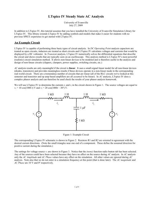
We will use LTspice IV to determine the currents i 1 and i 2 in the circuit shown in Figure 1. The source voltages are equal to
v 1 = 10 cos(1000 t) V and v 2 = 20 cos(1000t – 30º) V.
1 kΩ 1 H 1 H 1 kΩ
i 1
i 2
1 μF
v 1
+ + v – – 2
1 kΩ
Figure 1: Example Circuit
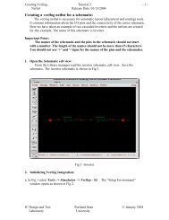
The corresponding LTspice IV schematic is shown in Figure 2. Resistors R1 and R2 are oriented in agreement with the
desired current directions. (Note the small triangles near one end of a component. These define the assumed direction for
positive current during the simulation.)
The settings for voltage source v 1 are shown in Figure 3. Notice that the (none) function radio button tab has been selected.
Any of the sources could have been selected because they have no affect on the source during AC analysis. In AC analysis
only the AC Amplitude and AC Phase values have any effect on the simulation. All other values are ignored during AC
analysis. Note also that we do not enter in a simulation frequency at this point (that is done later). The AC magnitude and
AC Phase are 10 V and 0º respectively.
1 of 5

Figure 2: LTspice IV Schematic
The voltage settings for v 2 look very similar except that the AC magnitude is equal to 20 and the AC Phase is equal to -30.
Figure 3: Voltage Source v 1 Settings
After completing the schematic and setting up the voltage sources. We are now ready to run an AC analysis. Click on the
Run icon and the Edit Simulation Command dialog window will appear as shown in Figure 4. Select the AC Analysis tab.
AC Analysis can be done at a single frequency or at several frequencies. We only want results at a single frequency
(1000 rad/s), so select List in the pull-down menu. In the text area at the bottom of the window add “{1000/(2*pi)}” to the
2 of 5

simulation command. (Note that LTspice IV expects frequencies in Hertz, not rad/sec. Now I could convert 1000 rad/s to
Hertz on my calculator, but I let LTspice IV do the calculation for me. As we have seen in previous tutorials, the expression
must be entered in curly braces.) After clicking on the OK button the simulation will proceed. A window similar to that
shown in Figure 5 should appear.
Figure 4: AC Analysis Simulation Command
From Figure 5 we see that the I 1 phasor is equal to (6.735 mA ∠38.5º) at 1000 rad/s while that of I 2 is equal to (5.946 mA
∠131.3º) These phasor values correspond to steady-state time-domain currents of:
i 1 = 6.735 cos(1000 t + 38.5º) mA
i 2 = 5.946 cos(1000 t + 131.3º) mA
Note that both phase angles are positive, so both currents lead voltage source v 1 .
Phasor Domain Circuits
You can use LTspice IV and AC analysis to obtain results for phasor domain circuits. Just set up the simulation at a
frequency of ω = 1 rad/s (f = 1/(2π) Hz). For an inductor with an impedance of jX use an inductance value of L = X in the
simulation. For a capacitor with an impedance of -jX use a capacitance value of C = 1/X. (Let LTspice IV do the math just
enclose the expression in curly braces).
For example to obtain V o in the phasor domain circuit shown in Figure 6, we use the LTspice IV schematic shown in Figure
7. At 1 rad/s (or 1/(2π) Hz), the components shown in the LTspice IV schematic will have exactly the same impedance as
the corresponding component in the phasor domain circuit. Results from simulating at a frequency of 1/(2π) Hz are shown
in Figure 8. The results indicate that V o is (11.314 V ∠-45º). Manual phasor domain analysis of the original circuit yields a
result of (11.314 V ∠-45º) in exact agreement with LTspice IV. (The LTspice IV simulation was much faster than manual
analysis!!)
3 of 5

Figure 5: AC Analysis Simulation Results
j70 Ω
-j400 Ω
72 V ∠0º
50 Ω
590 I X
I X
160 Ω
+
V O
-
Figure 6: Phasor Domain Circuit
Tips
You may have noticed that you can do the AC analysis at multiple frequencies. If you perform the AC analysis at more than
one frequency the Waveform Viewer will be opened and you then probe the circuit to display node voltages and device
currents as a function of frequency. This a very useful feature and will be the subject of the next tutorial.
4 of 5

--- AC Analysis ---
(a)
(b)
Figure 7: LTspice IV Schematic Corresponding to Figure 6
Note the inductance and capacitance values used in the schematic.
frequency: 0.159155 Hz
V(n002): mag: 30.4629 phase: -113.198° voltage
V(n003): mag: 41.7191 phase: 135.001° voltage
V(vo): mag: 11.3136 phase: -44.999° voltage
V(n004): mag: 30.4629 phase: -113.198° voltage
V(n001): mag: 72 phase: 0° voltage
I(C1): mag: 0.0707103 phase: 135.001° device_current
I(L1): mag: 1.2649 phase: -71.5641° device_current
I(R2): mag: 0.0707103 phase: -44.999° device_current
I(R1): mag: 1.20207 phase: -73.0715° device_current
I(V1): mag: 1.2649 phase: 108.436° device_current
Ix(u1:V+): mag: 1.20207 phase: -73.0715° subckt_current
Ix(u1:V-): mag: 1.20207 phase: 106.928° subckt_current
Ix(u1:ISAMPLE+): mag: 0.0707103 phase: 135.001° subckt_current
Ix(u1:ISAMPLE-): mag: 0.0707103 phase: -44.999° subckt_current
Figure 8: Results from Simulation of the Circuit in Figure 7
5 of 5