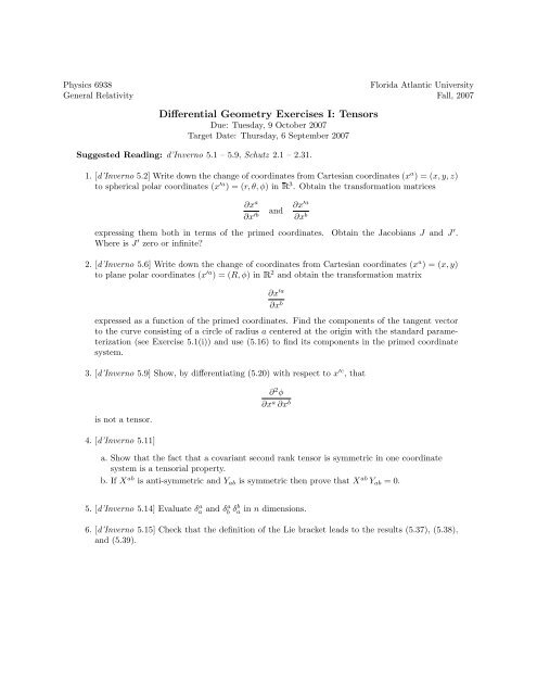
Differential Geometry Exercises I: Tensors - Fau.edu

Physics 6938
Florida Atlantic University
General Relativity Fall, 2007
Differential Geometry Exercises I: Tensors
Due: Tuesday, 9 October 2007
Target Date: Thursday, 6 September 2007
Suggested Reading: d’Inverno 5.1 – 5.9, Schutz 2.1 – 2.31.
1. [d’Inverno 5.2] Write down the change of coordinates from Cartesian coordinates (x a ) = (x, y, z)
to spherical polar coordinates (x ′a ) = (r, θ, φ) in R 3 . Obtain the transformation matrices
∂x a
∂x ′b
and
expressing them both in terms of the primed coordinates. Obtain the Jacobians J and J ′ .
Where is J ′ zero or infinite?
2. [d’Inverno 5.6] Write down the change of coordinates from Cartesian coordinates (x a ) = (x, y)
to plane polar coordinates (x ′a ) = (R, φ) in R 2 and obtain the transformation matrix
∂x ′a
∂x b
expressed as a function of the primed coordinates. Find the components of the tangent vector
to the curve consisting of a circle of radius a centered at the origin with the standard parameterization
(see Exercise 5.1(i)) and use (5.16) to find its components in the primed coordinate
system.
∂x ′a
∂x b
3. [d’Inverno 5.9] Show, by differentiating (5.20) with respect to x ′c , that
is not a tensor.
∂ 2 φ
∂x a ∂x b
4. [d’Inverno 5.11]
a. Show that the fact that a covariant second rank tensor is symmetric in one coordinate
system is a tensorial property.
b. If X ab is anti-symmetric and Y ab is symmetric then prove that X ab Y ab = 0.
5. [d’Inverno 5.14] Evaluate δ a a and δ a b δb a in n dimensions.
6. [d’Inverno 5.15] Check that the definition of the Lie bracket leads to the results (5.37), (5.38),
and (5.39).

7. [d’Inverno 5.16] In R 2 , let (x a ) = (x, y) denote Cartesian and (x ′a ) = (R, φ) plane polar
coordinates (see Exercise 5.6).
a. If the vector field X has components X a = (1, 0), then find X ′a .
b. The operator grad can be written in each coordinate system as
where f is an arbitrary function and
grad f = ∂f
∂x i + ∂f
∂y j = ∂f
∂R ˆR + ∂f
∂φ
ˆφ
R ,
ˆR = cos φ i + sin φ j, ˆφ = − sin φ i + cos φ j.
Take the scalar product of grad f with i, j, ˆR, and ˆφ in turn to find relationships
between the operators ∂/∂x, ∂/∂y, ∂/∂R, and ∂/∂φ.
c. Express the vector field X as an operator in each coordinate system. Use part (b) to
show that these expressions are the same.
d. If Y a = (0, 1) and Z a = (−y, x), then find Y ′a , Z ′a , Y , and Z.
e. Evaluate all the Lie brackets of X, Y and Z.
8. [Schutz 2.5 and 2.6, p. 59]
a. Prove that a general ( 2
0)
tensor cannot be expressed as a simple outer product of two
vectors.
(Hint: count the number of components a ( 2
0)
tensor may have.)
b. Prove that the ( 1
1)
tensor ¯V ⊗ ˜ω has components V i ω j .
c. Prove that the set of all ( 2
0)
tensors at P is a vector space under addition defined by
analogy with equation (2.16b). Show that ē i ⊗ ē j is a basis for that space. (Thus,
although a general ( 2
0)
tensor is not a simple outer product, it can be represented as a
sum of such tensors.) This vector space is called T P ⊗ T P .
9. [Schutz 2.8, p. 60] Let A and B be two ( 1
1)
tensors, and regard them as vector-valued linear
functions of vectors: if ¯V is a vector then A( ¯V ) and B( ¯V ) are vectors. Show that if we define
C( ¯V ) to be
C( ¯V ) = B(A( ¯V )),
then C is a ( 1
1)
tensor as well. Show that its components are
C i j = B i k A k j.
Discuss the relation of this with the linear transformation defined in §1.6.
10. [Schutz 2.13, p. 67]
a. Show that {g ij } are the components of a ( 2
0)
tensor g −1 , either by showing that they
transform properly, or that they define a bilinear function of one-forms.
b. Show that if a vector basis {ē i } is orthonormal, so is its dual one-form basis {˜ω i }, in
the sense that g −1 (˜ω i , ˜ω j ) = ±δ ij .

Physics 6938
Florida Atlantic University
General Relativity Fall, 2007
Differential Geometry Exercises II: Manifolds
Due: Tuesday, 9 October 2007
Target Date: Thursday, 13 September 2007
Suggested Reading: d’Inverno 6.1 – 6.2; Schutz 2.1 – 2.4 and 3.1 – 3.5.
1. [Schutz 3.1, p. 78]
a. Show that, on functions and fields,
[L ¯V , L ¯W ] = L [ ¯V , ¯W]
for any two twice-differentiable vector fields ¯V and ¯W .
b. Prove the Jacobi identity for Lie derivatives on functions and vector fields:
[[L ¯X, L Ȳ ] , L ¯Z] + [[L Ȳ , L ¯Z] , L ¯X] + [[L ¯Z, L ¯X] , L Ȳ ] = 0,
where ¯X, Ȳ , ¯Z are any three-times-differentiable vector fields.
Hint: For (a) on vectors, show that (3.8) is equivalent to (2.14). For (b) on vectors, use (3.8)
and the fact that, as is obvious from its definition, L Ā + L ¯B = L Ā+ ¯B.
2. [Schutz 3.2 and 3.3, p. 78]
a. Deduce the Leibniz rule
L ¯V (fŪ) = (L ¯V f) Ū + f L ¯V Ū
from the definitions of L ¯V on functions and vector fields.
b. From (2.7) we know that the components of L ¯V Ū on a coordinate basis are
(L ¯V Ū) i = V j ∂ ∂x j U i − U j ∂ ∂x j V i .
Given an arbitrary basis {ē i } for vector fields, show from (a) that
(L ¯V Ū) i = V j ē j (U i ) − U j ē j (V i ) + V j U k (Lēj ē k ) i ,
where ē j (U i ) means the derivative of the function U i with respect to the vector field ē j .
c. Show that if one chooses a coordinate system in which ¯V is a coordinate basis vector,
say ∂/∂x 1 , then for any vector field ¯W
(L ¯V ¯W ) i = ∂W i
∂x 1 .
That is, the Lie derivative is the coordinate-independent form of the partial derivative.
3. [Schutz 3.4, p. 79] From (3.13) and the expression (2.7) for the components of L ¯V ¯W =
[ ¯V , ¯W
]
,
deduce that L ¯V ˜ω has components, on a coordinate basis,
(L ¯V ˜ω) i = V j ∂ ∂x j ω i + ω j
∂
∂x i V j .

4. [d’Inverno 6.2] Use (6.17) to find expressions for L X Z bc and L X (Y a Z bc ). Use these expressions
and (6.15) to check the Leibniz property in the form (6.12).
5. Let (x, y, z) denote a point in R 3 with x 2 + y 2 + z 2 = 1. Define the maps
( )
x
ψ N (x, y, z) :=
1 + z , y
and ψ S (x, y, z) :=
1 + z
from S 2 to R 2 .
( x
1 − z , y
1 − z
a. Show that ψ N is defined everywhere on S 2 except at the south pole (0, 0, −1) and that
ψ S is defined everywhere except at the north pole (0, 0, 1).
b. Calculate the coordinate transformation ψ N ◦ ψ −1
S
(u, v) on the largest subset of R2 for
which it can be defined. Show that this mapping from R 2 to itself is smooth everywhere
it is defined.
c. Conclude that S 2 is a two-dimensional real manifold.
)
.
6. The complex projective plane CP 1 is the set of “complex lines” in C 2 — the set of vectors
(z 1 , z 2 ) ∈ C 2 up to overall scaling (z 1 , z 2 ) ↦→ (αz 1 , αz 2 ) by an arbitrary complex number α.
More mathematically, CP 1 is the set of equivalence classes [z 1 , z 2 ] of points in C 2 , where two
points are equivalent if and only if they are complex scalings of one another.
a. Define the mappings
ζ 1 := z1
z 2 and ζ 2 := z2
z 1
from C 2 to the complex plane C. Show that each is in fact a (complex) coordinate
chart mapping CP 1 to C.
b. What are the repsective domains U 1,2 of the charts ζ 1,2 ? That is, on what set of “lines”
[z 1 , z 2 ] ∈ CP 1 is each coordinate ζ 1,2 well-defined?
c. Show that the inverse charts mapping w ∈ C back to CP 1 can be written
ζ −1
1
(w) = [w, 1] and ζ−1 2 (w) = [1, w].
d. Find the coordinate transformation mapping the region ζ 1 (U 1 ∩U 2 ) of the complex plane
to the region ζ 2 (U 1 ∩ U 2 ) of the complex plane. Show that it is smooth and invertible
throughout ζ 1 (U 1 ∩ U 2 ), and that its inverse is also smooth. (In fact, it is analytic in
the complex-variables sense).
e. Conclude that CP 1 is a one-dimensional complex manifold.
7. Define the mapping
from S 2 to CP 1 .
φ(x, y, z) := [1 + z, x + iy] = [x − iy, 1 − z]
a. Prove the second equality in the above definition of φ(x, y, z).
b. Show that this mapping is invertible. That is, find a formula giving (x, y, z) as a
function of z 1 and z 2 , and check that this formula is invariant under scalings (z 1 , z 2 ) ↦→
(αz 1 , αz 2 ).
c. Calculate the four mappings ζ 1,2 ◦ φ ◦ ψ −1
N,S from R2 to C. Show that each is smooth
and has a smooth inverse.
d. Conclude that, viewed as a two-dimensional real manifold, CP 1 is diffeomorphic to S 2 .

Physics 6938
Florida Atlantic University
General Relativity Fall, 2007
Differential Geometry Exercises III: Connections
Due: Tuesday, 9 October 2007
Target Date: Tuesday, 25 September 2007
Suggested Reading: d’Inverno 6.3 – 6.12; Schutz 6.1 – 6.6.
1. [d’Inverno 6.5] Assuming (6.22) and (6.25), apply the Leibniz rule to the covariant derivative of
X a Y a , where Y a is arbitrary, to verify (6.26).
2. [d’Inverno 6.9] If s is an affine parameter, then show that, under the transformation
s ↦→ ¯s = ¯s(s),
the parameter ¯s will be affine if and only if ¯s = αs + β, where α and β are constants.
3. [d’Inverno 6.10] Show that ∇ c ∇ d X a b − ∇ d ∇ c X a b = R a ecd X e b − R e bcd X a e.
4. [d’Inverno 6.11] Show that ∇ X (∇ Y Z a ) − ∇ Y (∇ X Z a ) − ∇ [X,Y ] Z a = R a bcd Z b X c Y d .
5. [d’Inverno 6.14] The line elements of R 3 in Cartesian, cylindrical polar and spherical polar, and
spherical polar coordinates are given respectively by
ds 2 = dx 2 + dy 2 + dz 2 = dR 2 + R 2 dφ 2 + dz 2 = dr 2 + r 2 dθ 2 + r 2 sin 2 θ dφ 2 .
Find g ab , g ab and g in each case.
6. [d’Inverno 6.17] Find the geodesic equation for R 3 in cylindrical polars.
Hint: Use the results of Exercise 6.14 to compute the metric connection and substitute in (6.68).
7. [d’Inverno 6.20] Suppose we have an arbitrary symmetric connection Γ a bc satisfying ∇ c g ab = 0.
Deduce that Γ a bc
must be the metric connection.
Hint: Use the equation to find expressions for ∂ b g dc , ∂ c g db and −∂ d g bc , as in (6.78), add the
equations together and multiply by 1 2 gad .
8. [d’Inverno 6.23 and 6.24]
a. Establish the identities (6.78) and (6.79). Show that (6.78) is equivalent to R a [bcd] ≡ 0.
b. Establish the identity (6.82). Show that (6.82) is equivalent to R de[eb;c] ≡ 0. Deduce
(6.86).
Hint: Choose an arbitrary point P and introduce geodesic coordinates at P .
9. [Schutz 6.10, p. 208] Suppose a manifold has two connections defined on it, with Christoffel
symbols Γ k ij and Γ ′k ij. Show that
D k ij ≡ Γ k ij − Γ ′k ij
are the components of a ( 1
2)
tensor. Show that the tensor D is symmetric in its vector arguments
if and only if both connections have the same torsion tensor.

10. [Schutz 6.11, p. 208] A manifold has a symmetric connection. Show that in any expression for
the components of the Lie derivative, all commas can be replaced by semicolons. An example:
(L Ū ˜ω) i = ω i,j U j + ω j U j ,i = ω i;j U j + ω j U j ;i.
(Naturally, all commas must be changed, not just some.)
11. [Schutz 6.14, p. 211] The components of the Riemann tensor R i jkl, are defined by
[∇ i , ∇ j ] ē k − ∇ [ēi,ē j] ē k = R l kij ē l .
(Where ē i is possibly a non-coordinate basis. — CB)
a. Show that in a coordinate basis
R l kij = Γ l kj,i − Γ l ki,j + Γ m kj Γ l mi − Γ m ki Γ l mj.
b. In a non-coordinate basis, define the commutation coefficients C i jk by
Show that
where f ,i ≡ ē i [f].
c. Show that
[ē j , ē k ] = C i jk ē i .
R l kij = Γ l kj,i − Γ l ki,j + Γ m kj Γ l mi − Γ m ki Γ l mj − C m ij Γ l km,
R l k(ij) ≡ 1 2 (Rl kij + R l kji) = 0 and R l [kij] = 0.
Hint: For the second equality, use normal coordinates. The result, of course, is independent
of the basis.
d. Using (c) show that in an n-dimensional manifold, the number of linearly independent
components opf R l kij is
n 4 2 n(n + 1) n(n − 1)(n − 2)
− n − n = 1
2
3!
3 n2 (n 2 − 1).
12. [Schutz 6.16, p. 215] Consider a two-dimensional flat space with Cartesian coordinates x, y and
polar coordinates r, θ.
a. Use the fact that ē x and ē y are globally parallel vector fields (ē x (P ) is parallel to ē x (Q)
for arbitrary P , Q) to show that
Γ r θθ = −r, Γ θ rθ = Γ θ θr = 1 r ,
and all other Γ’s are zero in polar coordinates.
b. For an arbitrary vector field ¯V , evaluate ∇ i V j and ∇ i V i for polar cooridnates in terms
of the components V r and V θ .
c. For the basis
ˆr = ∂ ∂r , 1 ∂
ˆθ =
r ∂θ
find all the Christoffel symbols.
d. Same as (b) for the basis in (c).

Physics 6938
Florida Atlantic University
General Relativity Fall, 2007
Differential Geometry Exercises IV: Integration
Due: Tuesday, 9 October 2007
Target Date: Tuesday, 2 October 2007
Suggested Reading: d’Inverno 7.1 – 7.4; Schutz 4.1 – 4.23.
1. [d’Inverno 7.4] Show that, for any vector field T a , the divergence theorem in four dimensions
can be written in the form
∫
T a √ ∫
−g dS a = ∇ a T a √ −g d 4 x.
∂Ω
Ω
2. [Schutz 4.8, p. 118] Show that if ˜p is a one-form and ˜q a two-form, then
(˜p ∧ ˜q) ijk = p i q jk + p j q ki + p k q ij = 3 p [i q jk] .
More generally, show that if ˜p is a p-form and ˜q a q-form,
(˜p ∧ ˜q) i...jk...l = Cp p+q p [i...j q k...l] .
(The symbol C p+q
p
here is ( )
p+q
p from the binomial theorem. — CB)
3. [Schutz 4.9, p. 120] Prove (4.16).
4. [Schutz 4.12 and 4.13, pp. 131-132]
a. Show that the determinant of an n × n matrix with elements A ij (i, j = 1, . . . , n) is
det A = ɛ ij...k A 1i A 2j . . . A nk .
Hint: The determinant of an n × n matrix is defined in terms of (n − 1) × (n − 1)
determinants by the cofactor rule. Use that rule to prove this results by induction from
the 2 × 2 case.
b. Show that
det A = 1 n! ɛ ab...c ɛ ij...k A ai A bj . . . A ck .
c. If a manifold has a metric, let {˜ω i } be an orthonormal basis for one-forms, and define
˜ω to be the preferred volume-form
˜ω = ˜ω 1 ∧ ˜ω 2 ∧ . . . ∧ ˜ω n .
Show that, if x k′
is an arbitrary coordinate system,
˜ω = |g| 1/2 ˜dx
1 ′ ∧ ˜dx 2′ ∧ . . . ∧ ˜dx n′ ,
where g is the determinant of the matrix of components g i′ j ′
these coordinates.
of the metric tensor in

5. [Schutz 4.14, p. 135]
a. Show that
b. Use (a) to show that if
˜d(f ˜dg) = ˜df ∧ ˜dg.
˜α = 1 p! α i...j ˜dx i ∧ . . . ∧ ˜dx j
is the expansion for the p-form ˜α in a coordinate basis, then
˜d˜α = 1 p!
∂α i...j
∂x k ˜dx k ∧ ˜dx i ∧ . . . ∧ ˜dx j ,
and hence that (˜d˜α) ki...j = (p + 1) ∂ [k α i...j] .
6. [Schutz 4.16, p. 137] Use (4.50), (4.52), and property (iii) of §4.14 to show that (in threedimensional
Euclidean vector calculus) the divergence of a curl and the curl of a gradient both
vanish.
7. [Schutz 4.18, p. 142] Use the local exactness theorem to show that locally (in three-dimensional
Euclidean vector calculus) a curl-free vector field is a gradient and a divergence-free vector field
is a curl.
8. [Schutz 4.20 and 4.21, p. 148]
a. From (4.77) show that, if coordinates are chosen in which ˜ω = f ˜dx 1 ∧ . . . ∧ ˜dx n , then
div˜ω ¯ξ =
1
f (f ξi ) ,i .
b. In Euclidean three-space the preferred volume three-form is ˜ω = ˜dx ∧ ˜dy ∧ ˜dz. Show
that in spherical polar coordinates this is ˜ω = r 2 sin θ ˜dr ∧ ˜dθ ∧ ˜dφ. Use (4.80) to show
that the divergence of a vector ¯ξ = ξ r ∂ r + ξ θ ∂ θ + ξ φ ∂ φ is
div ¯ξ = 1 ∂
r 2 ∂r (r2 ξ r ) + 1 ∂
sin θ ∂θ (sin θ ξθ ) + ∂ξφ
∂φ .
9. [Schutz 4.23, p. 149]
a. Show from (4.77) that another expression for the divergence of a vector ¯ξ is
div˜ω ¯ξ = ∗d∗ ¯ξ,
where the ∗-operation is the dual with respect to ˜ω introduced earlier.
b. For any p-vector F define
div˜ω F = (−1) n(p−1) ∗d∗ F.
Show that div˜ω F is a (p − 1)-vector. Show that if ˜ω has components ɛ i...j in some
coordinate system, then
(div˜ω F) i...j = F ki...j ,k
in those coordinates.
c. Generalize part (a) of the previous exercise to p-vectors.

Physics 6938
Florida Atlantic University
General Relativity Fall, 2007
Differential Geometry Exercises V: Symmetry
Due: Tuesday, 9 October 2007
Target Date: Tuesday, 9 October 2007
Suggested Reading: d’Inverno 7.5 – 7.7; Schutz 3.6 – 3.13 and 5.11 – 5.14.
1. [d’Inverno 7.7] Use (7.45), (7.46), and (7.47) to find the geodesic equations of the spherically
symmetric line element given in Exercise 6.31. Use the equations to read off directly the components
Γ a bc
and check them with those obtained in Exercise 6.31(ii).
Hint: Remember Γ a bc = Γa cb .
2. [d’Inverno 7.12] Consider the following operator identity:
(U and V are vector fields. — CB)
L U L V − L V L U = L [U,V ] .
a. Check it holds when applied to an arbitrary scalar function f.
b. Check it holds when applied to an arbitrary contravariant vector field m a .
Hint: Use the Jacobi identity.
c. Deduce that the identity holds when applied to a covariant vector field p a .
Hint: Let f = m a p a , where m a is arbitrary.
d. Use the identity to prove that if U and V a Killing vector fields, then so is their
commutator [U, V ].
e. Given that ∂ x and −y ∂ x + x ∂ y are Killing vector fields, find another.
3. [d’Inverno 7.13 and 7.14]
a. By making use of the identity
R a bcd + R a cdb + R a dbc = 0
or otherwise, prove that a Killing vector satisfies
∇ c ∇ b X a = R abcd X d .
b. Use this result to prove that any Killing vector satisfies
g bc ∇ b ∇ c X a − R ab X b = 0.
4. [Schutz 6.20, p. 216] Show that for an arbitrary vector ¯V
(L ¯V g) ij = ∇ i V j + ∇ j V i .
Therefore a Killing vector obeys Killing’s equation ∇ (i V j) = 0.

5. [Schutz 3.5, p. 81]
a. Show that if ¯V and ¯W are linear combinations (not necessarily with constant coefficients)
of m vector fields that all commute with one another, then the Lie bracket of ¯V and ¯W
is a linear combination of the same m fields.
b. Prove the same result when the m vector fields have Lie brackets which are nonvanishing
linear combinations of the m fields.
6. Let ξ a be a Killing vector field for the metric g ab , and let η a be the tangent vector to a geodesic of
g ab in an affine parameterization. Show that the inner product of these vectors is constant along
the geodesic. What happens to this conserved quantity if one changes affine parameterizations?
What happens if the parameterization is not affine?
7. Let g ab be a stationary spacetime metric — meaning that it has a time-like Killing field t a —
that solves the vacuum Einstein equations R ab = 0.
a. Show that F ab := ∇ a t b satisfies the source-free Maxwell equations.
b. Suppose that t a is in fact a static Killing field — meaning that it is orthogonal everywhere
to some space-like surfaces Σ. Calculate the electric and magnetic parts of F ab
on the static slices Σ.
c. Use the Gauss law to compute the “electric charge” of the Schwarzschild metric
ds 2 = (1 − 2M/r) dt 2 + (1 − 2M/r) −1 dr 2 + r 2 (dθ 2 + sin 2 θ dφ 2 ).
Note that the static Killing field in this case is ∂ t , and that the static slices are the
surfaces of constant t in spacetime.
Hint: The electric charge is given by a flux integral. Show that one gets the same result
no matter which two-sphere one uses in the integral. Then, calculate in the asymptotic
region where r → ∞.