here - Alan Schoen geometry

Rules for the construction of symmetrical rhombic rosettes
Alan H. Schoen
0. INTRODUCTION
A rhombic rosette is an edge-to-edge tiling of the regular convex polygon {2n} by
⎛ n ⎞
⎜ ⎟
⎝ 2 ⎠
rhombs of ⎣n
/ 2⎦ different shapes. These ⎣n
/ 2⎦ rhombs, which we call the Standard Rhombic
Inventory SRI n , have smaller face angles kπ / n (1 ≤ k ≤ ⎣n
/ 2⎦ ); k is called the principal index of
the rhomb, and n − k is called its supplementary index (since the larger face angle of the rhomb is
( n − k) π / n).
We define each rhomb to have sides of unit length.
Rhombic rosettes have either
dihedral symmetry ds, where s is any odd divisor of n, or
cyclic symmetry cs, where s is any proper odd divisor of n.
Fig. 0.1 shows rosettes of five different symmetry types for n=9; Fig. 0.2 shows rosettes of four
different symmetry types for n=10. I describe below a systematic procedure that facilitates the
construction of both dihedral and cyclic rosettes ‘by hand’, i.e., by arranging paper rhombs.
d9 d3 d1 c3 c1
Fig. 0.1
Rhombic rosettes for n=9
d5 d1 c5 c1
Fig. 0.2
Rhombic rosettes for n=10
1

1. DIHEDRAL ROSETTES
A dihedral rosette with symmetry ds contains s diametral pendants—linear strings of rhombs
bounded by opposite boundary vertices. Each such pendant is symmetrical by reflection in its
axis—a circumdiameter that is one of the s lines of reflection of the rosette. Figs. 1.1-1.2 show a
d9
rosette and a d 5 rosette, together with their diametral pendants and diametral index strings
(defined below).
2
6
(a) (b) (c) (d)
Fig. 1.1. (a) d9 rosette; (b) one diametral pendant; (c) pendant index string; (d) the nine diametral pendants
8
4
0
(a) (b) (c) (d)
Fig. 1.2. (a) d5 rosette; (b) one diametral pendant; (c) pendant index string; (d) the five diametral pendants
For each rhomb in a diametral pendant, vertices that lie on the pendant axis are called axial
vertices, and the face-angle index at an axial vertex is called an axial index. If the axial vertices of
a rhomb are even, the rhomb is called even; otherwise it is called odd. The sequence of
⎣( n + 1) / 2⎦ axial indices for the ⎣( n + 1) / 2⎦ rhombs of a diametral pendant is called the
diametral index string. Examples of these strings are shown in Figs. 1.1c and 1.2c.
Every diametral pendant for s ≥ 3 is partitioned at the center of the rosette into two radial
pendants of equal projected length but different composition. Hence the diametral index string is
the union of two complementary substrings called radial index strings.
An efficient method of designing a dihedral rosette by hand is to construct the radial pendants
first and then fill in the sectors between them. Except in the case of small n, however, it is not
obvious which rhombs to assign to the two radial pendants and how to orient them. This note
describes a systematic procedure that is conjectured to define, for all n ≥ 3, the composition of
every possible pair of complementary radial pendants. The arrangement of the rhombs in each
radial pendant is left unspecified (but see the hint below).
2
9
7
1
3
5

A diametral pendant is composed of n/2 odd rhombs if n is even, and of (n+1)/2 even
rhombs— including one zero rhomb, defined as a line segment of unit length—if n is odd.
I conjecture that for every partition of diametral rhombs generated by the procedure described
below, there exists at least one dihedral rosette with radial pendants of composition defined by the
partition. Although I have confirmed the truth of this conjecture in every example tested, I have
not succeeded in constructing a general proof. Experience shows that once a pendant partition has
been selected, it is not difficult to discover compatible arrangements of rhombs in the radial
pendants, i.e., arrangements that allow the rosette tiling to be completed. It may be possible to
predict precisely which such sequences are compatible, but I do not know how to do this.
A hint about one kind of compatible arrangement of the rhombs in radial pendants is suggested
by the dihedral rosettes in Figs. 0.1 and 0.2: Let axial indices increase from the center outward.
Procedure for partitioning a diametral pendant into two radial pendants A and B
(a) n is even
s is any odd divisor ≥ 3 of n
(i) Construct a n / 2 x 2 matrix of bins: two rows—A and B—and n / 2 columns, each headed by
the name of one of the n / 2 axial indices 1, 3, 5, …, n-3, n-1. The procedure will assign axial
indices to the bins in a variety of different arrangements.
A
B
1 3 5 n-5 n-3 n-1
1
Axial indices assigned to row A are denoted as
denoted as k
j
(1 ≤ j ≤ β ), where α + β = n / 2.
k (1 ≤ i ≤ α );
i
those assigned to row B are
Let K = { k1, k2, ..., k α
} = the set of α axial indices assigned to row A, and
K = { k
1, k
2,..., k β
} = the set of β axial indices assigned to row B.
The solution set K of entries in row A defines a radial index string, and the solution set K in row
B defines its complement. The union K ∪ K = the set {1, 3, 5, …, n-1} of α + β ( = n / 2 ) axial
indices in the diametral index string.
(ii) Define a “sum relation” to be an equation of type
2n
ki
+ k
j
=
s
(1 ≤ i ≤ α ; 1 ≤ j ≤ β )
(1.1)
and a “difference relation” to be an equation of type
2n
ki
− k
j
=
s
(1 ≤ i ≤ α ; 1 ≤ j ≤ β ).
(1.2)
3

(iii) Place axial index 1 in the leftmost bin of row A. Then assign each of the remaining indices
either to row A or to row B, in every arrangement that contains σ sum relations and δ difference
relations, where
n
σ = (1.3)
2s
n
δ = ( s − 2).
(1.4)
(b) n is odd
s is any odd divisor ≥ 3 of n
2s
(i) Construct a ( n + 1) / 2 x 2 matrix of bins: two rows—A and B—and ( n + 1) / 2 columns, each
headed by the name of one of the axial indices 0, 2, 4, …, n-3, n-1. The procedure will assign axial
indices to the bins in a variety of different arrangements.
A
B
0 2 4 n-5 n-3 n-1
0
Axial indices assigned to row A are denoted as
denoted as k
j
(1 ≤ j ≤ β ), where α + β = n / 2.
k (1 ≤ i ≤ α );
i
those assigned to row B are
Let K = { k1, k2, ..., k α
} = the set of α axial indices assigned to row A, and
K = { k
1, k
2,..., k β
} = the set of β axial indices assigned to row B.
The solution set K of entries in row A defines a radial index string, and the solution set K in row
B defines its complement. The union K ∪ K = the set {0, 2, 4, …, n-1} of α + β = ( n + 1) / 2
axial indices in the diametral index string.
(ii) Define a “sum relation” to be an equation of type
2n
ki
+ k
j
= (1 ≤ i ≤ α ; 1 ≤ j ≤ β )
(1.5)
s
and a “difference relation” an equation of type
2n
ki
− k
j
= (1 ≤ i ≤ α ; 1 ≤ j ≤ β )
(1.6)
s
(iii) Place axial index 0 in the leftmost bin in row A. Then assign each of the remaining indices
either to row A or to row B, in every arrangement that contains σ sum relations and δ difference
relations, where
n 1
σ = + (1.7)
2s
2
n 1
δ = ( s − 2) + . (1.8)
2s
2
4

(Reminder: The projected length λ of a rhomb on the pendant axis is equal to 2cos( θ / 2),
where θ the face angle of a pendant rhomb at each of its axial vertices.)
Let s be any odd divisor ≥ 3 of n. Then every pair of complementary solution sets K and K
satisfies the equation
α β
π π
∑cos ki
= ∑ cos k
j
(1.9)
2n
2n
i= 1 j=
1
= r / 2 (1.10)
where r, the inradius of the rosette, is
⎛ 1 ⎞ π
r = ⎜ ⎟csc
. (1.11)
⎝ 2 ⎠ 2n
_______________________________________________________________________________
The number of solution sets
Let P(n,s) = the number of solution sets for a rosette of order n ≥ 3 and dihedral symmetry ds
(s ≥ 3). Then
P(n,s) = 2 s-1
(1.12)
Proof (even n)
After the ‘1’ is assigned (without loss of generality) to row A in the first column of bins, there
remain 2 s-1 distinct ways to assign indices in the next 1 σ − columns, i.e., the columns for
indices 3, 5, …, 2σ − 1.
Let
2 n
ω = ( = 4 σ ).
(1.13)
s
The assigning of indices to the next σ columns, i.e., the columns for
indices 2σ + 1, 2σ + 3, ..., 4σ − 3, 4σ
− 1,
is dictated by the σ sum relations (Eq. 1.5):
1 + 4σ
− 1=
ω
3 + 4σ
− 3=
ω
…
2σ − 3+ 2σ + 3 = ω
2σ − 1+ 2σ + 1 = ω
(1.14)
5

n
The assigning of indices to the last − 2σ
= δ columns, i.e., the columns for
2
indices 4σ
+ 1, 4σ
+ 3, ..., n − 1,
is dictated by the δ difference relations (cf. Eq. 1.6). Hence the 2 s-1 distinct ways of assigning
indices to the first σ columns exhaust all possibilities.
(The proof for odd n is left to the reader.)
______________________________________________________________________________
The composition of the pairs of complementary radial pendants is displayed in graphical form
in Figs. 1.3-1.5 for ( n, s ) = (24,3), (27,3), and (30,3). These diagrams illustrate how complete
solution sets are derived from the first σ columns by combining the elementary symmetry
operations (a) translation, (b) reflection, and (c) inversion (i.e., reflection followed by exchange of
rows).
1 3 5 7 9 11 13 15 17 19 21 23
0 2 4 6 8 10 12 14 16 18 20 22 24 26
Hn,sL = H24,3L
Hn,sL = H27,3L
Fig. 1.3 Fig. 1.4
1 3 5 7 9 11 13 15 17 19 21 23 25 27 29
Hn,sL = H30,3L
Fig. 1.5
Appendix 1 lists every possible solution set for 3 ≤ n ≤ 30 , for all allowed values of s.
6

2. CYCLIC ROSETTES
The sequence of rhombs in every ladder is described by a ladder string—an ordered list of the
n − 1 ladder indices k of the face angles k π / n ( k ∈[1, n −1])
at the lower left corners of the ladder
rhombs.
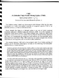
Figs. 2.1 and 2.2 show two examples of a c3 rosette. The
indiameter perpendicular to each ladder’s rungs (edges
common to adjacent rhombs in the ladder) is called the axis
of the ladder (cf. dashed line in Fig. 2.1). Six of the nine
ladders of this c3 rosette are balanced, i.e., they are
partitioned at the center of the rosette into complementary
half-ladders, each of which has projected length on the
ladder axis equal to the inradius r = 1 / ( 2 tan ( π / 2 n).
In
Fig. 2.1
every rosette with cyclic symmetry cs (s=odd integer ≥ 3)
there are at least s balanced ladders.
A c3 rosette (n=9) and a balanced ladder
Designing a cyclic rosette by hand begins with the
balanced ladder algorithm—a recipe for (I) deriving every
possible composition of two complementary half-ladders and
(II) specifying the orientation of all the non-square rhombs
(i.e., whether they ‘lean’ to the left or to the right). After the
n − 1 rhombs are arranged in a particular sequence, s
congruent replicas of the ladder are placed inside the tiling
arena. Finally the remaining rhombs in SRI n are used to tile
the sectors between the s ladders.
The string for the balanced ladder in Fig 2.1 is {8,1,2,3,7 | 4,6,5}.
The strings for the balanced ladders at the bottom of Fig. 2.2,
beginning with the darker half-ladder, are:
{17,13,1,2,3,5,6,10,14,15 | 4,9,8,12,7,11,16} (left)
{1,2,6,9,10,11,13,14 | 5,4,8,7,3,12,15,16,17} (middle)
{1,17,16,4,5,6,8,9,13 | 3,2,7,12,11,15,10,14} (right)
Fig. 2.2
Top: A c3 rosette (n=18)
Bottom: Three balanced ladders, partitioned at the center of the rosette into two half-ladders of equal projected length
7

The balanced ladder algorithm
I. Assigning the n - 1 ladder rhombs to two complementary half-ladders
Let n = a composite positive integer≥ 6 and s = any proper odd divisor ≥ 3 of n:
n = s q. (2.1)
(i) First construct the skeletal sequence, composed of s terms with increment q.
(a) s ≡ 1 (mod 4 µ ) ( µ = 1, 2 ,...)
The skeletal sequence is:
1
0 q 2 q 3 q … ( s − 1)
q
2
1
( s + 1) terms
2
14243
1
| q 2 q 3 q … ( s − 1)
q
2
1
| ( s − 1) terms
2 14243
(2.2)
( s terms altogether)
1442443
(b) s ≡ −1 (mod 4 µ ) ( µ = 1, 2 ,...)
The skeletal sequence is:
1
0 q 2 q 3 q … ( s − 1)
q
2
1
( s + 1) terms
2 14243
1
| q 2 q 3 q … ( s − 1)
q
2
1
| ( s − 1) terms
2 14243
(2.3)
( s terms altogether)
1442443
Upper and lower bars are assigned consecutively to the terms on each side of (2.2) and (2.3):
Place a bar above term 1, below term 2, above term 3, … (etc.).
An upper bar means add 1 to the term; a lower bar means subtract 1 from the term.
(Repeat this procedure, so long as no term becomes greater than n / 2 .)
For example, for (n,s,q) = (18,9,2), the skeletal sequence is 0 2 4 6 8 | 2 4 6 8 .
Applying the bar rule yields 1 1 5 5 9 | 3 3 7 7 , which is called a basic exchange relation.
For (n,s,q) = (18,3,6), the skeletal sequence is 0 6 | 6 . Applying the bar rule three times in
succession (while keeping all the bars in the same positions) yields three basic exchange relations
1 5 | 7 , 2 4 | 8 , and 3 3 | 9 .
A basic exchange relation describes the composition of two matched ribbons of rhombs,
i.e., ribbons of equal projected length.
It enables the transfer of rhombs between matched half-ladders.
8

The basic exchange relation 1 1 5 5 9 | 3 3 7 7 for ( n, s, q ) = ( 18, 9, 2 ), is equivalent to
sin( 1π / 18) + sin( 1π / 18) + sin( 5π / 18) + sin( 5π / 18) + sin( 9 π / 18)
=
sin( 3π / 18) + sin( 3π / 18) + sin( 7π / 18) + sin( 7 π / 18),
or
2sin( π / 18) + 2sin( 5π / 18) + sin( 9π / 18) = 2sin( 3π / 18) + 2sin( 7π
/ 18 ) . (2.4)
The matched ribbons of rhombs in Fig. 2.3 illustrate this exchange relation.
1 1 5 5 9 3 3 7 7
Fig. 2.3
The basic exchange relations 1 5 | 7 , 2 4 | 8,
and 3 3 | 9 for ( n, s, q ) = ( 18, 3, 6 ) are equivalent
to
sin( π / 18) + sin( 5π / 18) = sin( 7π
/ 18 ),
(2.5a)
sin( π / 9) + sin( 2π / 9) = sin( 4π
/ 9),
and (2.5b)
2sin( π / 6) = sin( π / 2 ), respectively. (2.5c)
The matched ribbons of rhombs in Fig. 2.4 illustrate the basic exchange relations (2.5a), (2.5b), and
(2.5c).
1 5 7 2 4 8 3 3 9
Fig. 2.4
For ( n, s, q ) = ( 9, 3, 3),
there is only one exchange relation: 1 2 | 4 , which is equivalent to the
exchange relation 2 4 | 8 for ( n, s, q ) = ( 18, 3, 6 ) (cf. Fig 2.4).
The result of applying two or more basic exchange relations in succession is equivalent to
applying a composite exchange relation.
For example, 1 5 | 7 + 2 4 | 8 ≡ 1 5 2 4 | 7 8
and 1 5 | 7 + 8 | 2 4 ≡ 1 5 8 | 7 2 4 .
9

(ii) Construct a standard pair of matched half-ladders if n is odd, and
a standard pair of truncated half-ladders if n is even.
Then apply one or more basic exchange relations, thereby producing matched half-ladder strings.
For odd n, each of the two matched half-ladder strings of the standard pair in (2.7) contains the
index for every shape of rhomb in SRI n :
{ 1, 2, ... , ( n − 1) / 2} | { 1, 2, ... , ( n − 1) / 2 }.
(2.7)
For even n, producing a standard pair of matched half-ladder strings requires three steps. We
illustrate with an example. Consider ( n, s, q ) = ( 18, 9, 2 ).
(a) First construct a pair of identical truncated strings, each containing the index for every
rhomb except the square:
{ 1, 2, ... , 8} | { 1, 2, ... , 8 }.
(2.8)
(b) Apply the basic exchange relation ERS that contains the square, 1 1 5 5 9 | 3 3 7 7 , to
each string in (2.8). This means adding the rhombs on the left side of ERS to the left side of
(2.8) and adding the rhombs on the right side of ERS to the right side of (2.8):
3 3 3 3
{ 1 , 2, 3, 4, 5 , 6, 7, 8, 9} | { 1, 2, 3 , 4, 5, 6, 7 , 8}
1
(c) Because the number of non-square rhombs in a ladder is limited to two, reduce the halfladder
strings in (2.9) by removing all extra indices:
2 2 2 2
{ 1 , 2, 4, 5 , 6, 8, 9} | { 2, 3 , 4, 6, 7 , 8 }
(2.10)
(2.10) is the required standard pair of matched half-ladder strings for ( n, s, q ) = ( 18, 9, 2 ).
As a second example, consider ( n, s, q ) = ( 18, 3, 6 ) (cf. Fig. 2.2). Because n is even, steps (ii-a)
and (ii-b) require that the exchange relation 3 3 | 9 be applied to the identical truncated strings
{ , , ... , } | { , , ... , }
1 2 8 1 2 8 in (2.8), yielding
3
{ 1, 2, 3 , 4, 5, 6, 7, 8} | { 1, 2, 3, 4, 5, 6, 7, 8, 9 }.
(2.11)
After reduction, (2.11) is transformed into the standard pair
2
{ 1, 2, 3 , 4, 5, 6, 7, 8} | { 1, 2, 4, 5, 6, 7, 8, 9 }.
(2.12)
If the exchange relation 1 5 | 7 were applied to (2.12), the result would be
2 2 2 2
{ 1 , 2, 3 , 4, 5 , 6, 8} | { 2, 4, 6, 7 , 8, 9 },
(2.13)
which defines the complementary half-ladders shown at bottom left in Fig. 2.2.
_____________________________________________________________________________
Every possible balanced ladder composition can be obtained by repeated application of basic
exchange relations. If there are altogether m basic exchange relations, they can be combined to
produce a total of ( 3 m − 1) / 2 exchange relations (including both basic and composite relations).
1
The notation index j above means that there are j instances of the rhomb with index index.
10

II. Specifying the orientation of the non-square rhombs in two complementary half-ladders
4
7
8
2
9
7
3
6
4
8
Part I of the balanced ladder algorithm explained how to choose
sets of rhombs that form connected ribbons that have the overall
length required for a half-ladder. Because a circle inscribed in a
regular polygon is tangent to the polygon at the midpoint of each
polygon edge, in a balanced ladder there is a lateral offset—equal to
one-half of the rhomb edge length—between the end rung of each
half-ladder and the center of the rosette (cf. Fig. 2.5). Since the
rhombs of each identical pair in a half-ladder are oppositely oriented
(they are related by a glide reflection), they make no contribution to
this lateral offset. It is the relative orientations of all the singleton
rhombs in the half-ladder that accounts for the offset.
1
2
5
Fig. 2.5
A balanced ladder for n=18
3
1
5
6
A simple procedure that specifies the orientations of the singleton
rhombs is the zigzag rule (described below). The zigzag rule is a
special case of a more general procedure called ‘p-fold q-chains’,
which was discovered by closely examining the balanced ladders in a
variety of computer-generated rosettes. In 1980, Andy Odlyzko
(personal communication) proved the validity of the p-fold q-chains
rule. A description of the rule, including Odlyzko’s proof, will be
published on the author’s website, schoengeometry.com.)
The zigzag rule:
1. Assign a rank from 1 to g to each of the g singletons in the half-ladder, in order of size.
2. Let the rhombs of even rank lean left and those of odd rank lean right (or vice versa).
In each of the half-ladders of Fig. 2.5, there are four singletons, with principal indices 2, 4, 6, 8.
It is apparent that their orientations are consistent with the zigzag rule.
______________________________________________________________________________
This summary is an edited version of the author’s report Rhombic Rosettes, issued in 1979 by the
Dept. of Design, Southern Illinois University/Carbondale.
11

APPENDIX 1
Diametral pendant partitions (3 ≤ n ≤ 30)
s=3 P(3,3)=1 ( σ , δ , ω ) = (1,1,2)
(1) 0
n=3
2
s=5 P(5,5)=1 ( σ , δ , ω ) = (1,2,2)
n=5
(1) 0 4
2
s=3 P(6,3)=1 ( σ , δ , ω ) = (1,1,4)
(1) 1
n=6
3 5
s=7 P(7,7)=1 ( σ , δ , ω ) = (1,3,2)
n=7
(1) 0 4
2 6
s=3 P(9,3)=2 ( σ , δ , ω ) = (2,2,6)
n=9
(1) 0 2
4 6 8
____________________________________________________________________________
(2) 0 4 8
2 6
____________________________________________________________________________
s=9 P(9,9)=1 ( σ , δ , ω ) = (1,4,2)
(1) 0 2
4 6 8
13

s=5 P(10,5)=1 ( σ , δ , ω ) = (1,3,4)
n=10
(1) 1 7 9
3 5
s=11 P(11,11)=1 ( σ , δ , ω ) = (1,5,2)
n=11
(1) 0 4 8
2 6 10
s=3 P(12,3)=2 ( σ , δ , ω ) = (2,2,8)
n=12
(1) 1 3
5 7 9 11
____________________________________________________________________________
(2) 1 5 11
3 7 9
s=13 P(13,13)=1 ( σ , δ , ω ) = (1,6,2)
n=13
(1) 0 4 8 12
2 6 10
s=7 P(14,7)=1 ( σ , δ , ω ) = (1,5,4)
n=14
(1) 1 7 9
3 5 11 13
s=3 P(15,3)=4 ( σ , δ , ω ) = (3,3,10)
n=15
(1) 0 2 4
6 8 10 12 14
____________________________________________________________________________
14

n=15 (cont.)
(2) 0 2 6 14
4 8 10 12
____________________________________________________________________________
(3) 0 6 8 12 14
2 4 10
____________________________________________________________________________
(4) 0 4 8 12
2 6 10 14
____________________________________________________________________________
s=5 P(15,5)=2 ( σ , δ , ω ) = (2,5,6)
(1) 0 2 10 12 14
4 6 8
____________________________________________________________________________
(2) 0 4 8 12
2 6 10 14
____________________________________________________________________________
s=15 P(15,15)=1 ( σ , δ , ω ) = (1,7,2)
(1) 0 4 8 12
2 6 10 14
s=17 P(17,17)=2 ( σ , δ , ω ) = (1,8,2)
n=17
(1) 0 4 8 12 16
2 6 10 14
s=3 P(18,3)=4 ( σ , δ , ω ) = (3,3,12)
n=18
(1) 1 3 5
7 9 11 13 15 17
____________________________________________________________________________
(2) 1 3 7 17
5 9 11 13 15
____________________________________________________________________________
15

n=18 (cont.)
(3) 1 5 9 15
3 7 11 13 17
____________________________________________________________________________
(4) 1 7 9 15 17
3 5 11 13
____________________________________________________________________________
s=9 P(18,9)=1 ( σ , δ , ω ) = (1,7,4)
) 1 7 9 15 17
3 5 11 13
s=19 P(19,19)=1 ( σ , δ , ω ) = (1,9,2)
n=19
(1) 0 4 8 12 16
2 6 10 14 18
s=5 P(20,5)=2 ( σ , δ , ω ) = (2,6,8)
n=20
(1) 1 5 11 15 17
3 7 9 13 19
____________________________________________________________________________
(2) 1 3 13 15 17 19
5 7 9 11
s=3 P(21,3)=8 ( σ , δ , ω ) = (4,4,14)
n=21
(1) 0 2 4 6
8 10 12 14 16 18 20
____________________________________________________________________________
(2) 0 2 4 8 20
6 10 12 14 16 18
____________________________________________________________________________
(3) 0 2 6 10 18
4 8 12 14 16 20
____________________________________________________________________________
16

n=21 (cont.)
(4) 0 4 8 12 16 20
2 6 10 14 18
___________________________________________________________________________
(5) 0 2 8 10 18 20
4 6 12 14 16
____________________________________________________________________________
(6) 0 2 4 6
8 10 12 14 16 18 20
____________________________________________________________________________
(7) 0 6 10 12 16 18
2 4 8 14 20
____________________________________________________________________________
(8) 0 8 10 12 16 18 20
2 4 6 14
____________________________________________________________________________
s=7 P(21,7)=2 ( σ , δ , ω ) = (2,8,6)
(1) 0 2 10 12 14
4 6 8 16 18 20
____________________________________________________________________________
(2) 0 4 8 12 16 20
2 6 10 14 18
____________________________________________________________________________
s=21 P(21,21)=1 ( σ , δ , ω ) = (1,10,2)
(1) 0 4 8 12 16 20
2 6 10 14 18
s=11 P(22,11)=1 ( σ , δ , ω ) = (1,9,4)
n=22
(1) 1 7 9 15 17
3 5 11 13 19 21
17

s=23 P(23,23)=1 ( σ , δ , ω ) = (1,11,2)
n=23
(1) 0 4 8 12 16 20
2 6 10 14 18 22
s=3 P(24,3)=1 ( σ , δ , ω ) = (4,4,16)
n=24
(1) 1 3 5 7
9 11 13 15 17 19 21 23
_________________________________________________________________________________
(2) 1 3 5 23
7 9 11 13 15 17 19 21
____________________________________________________________________________________
(3) 1 3 7 11 21
5 9 13 15 17 19 23
____________________________________________________________________________________
(4) 1 5 7 13 19
3 9 11 15 17 21 23
____________________________________________________________________________________
(5) 1 3 9 11 21 23
5 7 13 15 17 19
____________________________________________________________________________________
(6) 1 5 9 13 17 21
3 7 11 15 19 23
____________________________________________________________________________________
(7) 1 7 11 13 19 21
3 5 9 15 17 23
____________________________________________________________________________________
(8) 1 9 11 13 19 21 23
3 5 7 15 17
18

s=5 P(25,5)=4 ( σ , δ , ω ) = (3,8,10)
n=25
(1) 0 2 4 16 18 20 22 24
6 8 10 12 14
_______________________________________________________________________________
(2) 0 2 6 14 18 20 22
4 8 10 12 16 24
_______________________________________________________________________________
(3) 0 4 8 12 16 20 24
2 6 10 14 18 22
_______________________________________________________________________________
(4) 0 6 8 12 14 20
2 4 10 16 18 22 24
s=13 P(26,13)=1 ( σ , δ , ω ) = (1,11,4)
n=26
(1) 1 7 9 15 17 23 25
3 5 11 13 19 21
s=3 P(27,3)=16 ( σ , δ , ω ) = (5,5,18)
n=27
(1) 0 2 4 6 8
10 12 14 16 18 20 22 24 26
_______________________________________________________________________________
(2) 0 2 4 6 10 26
8 12 14 16 18 20 22 24
_______________________________________________________________________________
(3) 0 2 4 8 12 24
6 10 14 16 18 20 22 26
_______________________________________________________________________________
(4) 0 2 6 8 14 22
4 10 12 16 18 20 24 26
_______________________________________________________________________________
(5) 0 4 6 8 16 20
2 10 12 14 18 22 24 26
19

_______________________________________________________________________________
n=27 (cont.)
(6) 0 2 4 10 12 24 26
6 8 14 16 18 20 22
________________________________________________________________________________
(7) 0 2 6 10 14 22 26
4 8 12 16 18 20 24
________________________________________________________________________________
(8) 0 4 6 10 16 20 26
2 8 12 14 18 22 24
________________________________________________________________________________
(9) 0 2 8 12 14 22 24
4 6 10 16 18 20 26
________________________________________________________________________________
(10) 0 4 8 12 16 20 24
2 6 10 14 18 22 26
________________________________________________________________________________
(11) 0 6 8 14 16 20 22
2 4 10 12 18 24 26
________________________________________________________________________________
(12) 0 2 10 12 14 22 24 26
4 6 8 16 18 20
________________________________________________________________________________
(13) 0 4 10 12 16 20 24 26
2 6 8 14 18 22
________________________________________________________________________________
(14) 0 6 10 14 16 20 22 26
2 4 8 12 18 24
________________________________________________________________________________
(15) 0 8 12 14 16 20 22 24
2 4 6 10 18 26
________________________________________________________________________________
(16) 0 10 12 14 16 20 22 24 26
2 4 6 8 18
________________________________________________________________________________
20

s=9 P(27,9)=2 ( σ , δ , ω ) = (2,11,6)
n=27 (cont.)
(1) 0 2 10 12 14 22 24 26
4 6 8 16 18 20
________________________________________________________________________________
(2) 0 4 8 12 16 20 24
2 6 10 14 18 22 26
________________________________________________________________________________
s=9 P(27,27)=1 ( σ , δ , ω ) = (1,13,2)
(1) 0 4 8 12 16 20 24
2 6 10 14 18 22 26
s=7 P(28,7)=2 ( σ , δ , ω ) = (2,10,8)
(1) 1 3 13 15 17 19
5 7 9 11 21 23 25 27
________________________________________________________________________________
(2) 1 5 11 15 17 21 27
3 7 9 13 19 23 25
s=7 P(29,29)=1 ( σ , δ , ω ) = (1,14,2)
n=29
(1) 0 4 8 12 16 20 24 28
2 6 10 14 18 22 26
________________________________________________________________________________
s=3 P(30,3)=16 ( σ , δ , ω ) = (5,5,20)
n=30
(1) 1 3 5 7 9
11 13 15 17 19 21 23 25 27 29
________________________________________________________________________________
(2) 1 3 5 7 11 29
9 13 15 17 19 21 23 25 27
________________________________________________________________________________
(3) 1 3 5 9 13 27
7 11 15 17 19 21 23 25 29
21

n=30 (cont.)
(4) 1 3 7 9 15 25
5 11 13 17 19 21 23 27 29
________________________________________________________________________________
(5) 1 5 7 9 17 23
3 11 13 15 19 21 25 27 29
________________________________________________________________________________
(6) 1 3 5 11 13 27 29
7 9 15 17 19 21 23 25
________________________________________________________________________________
(7) 1 3 7 11 15 25 29
5 9 13 17 19 21 23 27
________________________________________________________________________________
(8) 1 5 7 11 17 23 29
3 9 13 15 19 21 25 27
________________________________________________________________________________
(9) 1 3 9 13 15 25 27
5 7 11 17 19 21 23 29
________________________________________________________________________________
(10) 1 5 9 13 17 21 25 29
3 7 11 15 19 23 27
________________________________________________________________________________
(11) 1 7 9 15 17 23 25
3 5 11 13 19 21 27 29
________________________________________________________________________________
(12) 1 3 11 13 15 25 27 29
5 7 9 17 19 21 23
________________________________________________________________________________
(13) 1 5 11 13 17 23 27 29
3 7 9 15 19 21 25
________________________________________________________________________________
(14) 1 7 11 15 17 23 25 29
3 5 9 13 19 21 27
________________________________________________________________________________
(15) 1 9 13 15 17 23 25 27
3 5 7 11 19 21 29
________________________________________________________________________________
22

n=30 (cont.)
(16) 1 11 13 15 17 23 25 27 29
3 5 7 9 19 21
________________________________________________________________________________
s=5 P(30,5)=4 ( σ , δ , ω ) = (3,9,12)
(1) 1 3 5 19 21 23 25 27 29
7 9 11 13 15 17
________________________________________________________________________________
(2) 1 3 7 17 21 23 25 27
5 9 11 13 15 19 29
________________________________________________________________________________
(3) 1 5 9 15 17 19 23 25 29
3 7 11 13 21 27
________________________________________________________________________________
(4) 1 7 9 15 17 23 25
3 5 11 13 19 21 27 29
________________________________________________________________________________
s=15 P(30,15)=1 ( σ , δ , ω ) = (1,13,4)
(1) 1 7 9 15 17 23 25
3 5 11 13 19 21 27 29
_______________________________________________________________________________
23